Abstract
This paper addresses the automated segmentation of multiple organs in upper abdominal computed tomography (CT) data. The aim of our study is to develop methods to effectively construct the conditional priors and use their prediction power for more accurate segmentation as well as easy adaptation to various imaging conditions in CT images, as observed in clinical practice. We propose a general framework of multi-organ segmentation which effectively incorporates interrelations among multiple organs and easily adapts to various imaging conditions without the need for supervised intensity information. The features of the framework are as follows: (1) A method for modeling conditional shape and location (shape–location) priors, which we call prediction-based priors, is developed to derive accurate priors specific to each subject, which enables the estimation of intensity priors without the need for supervised intensity information. (2) Organ correlation graph is introduced, which defines how the conditional priors are constructed and segmentation processes of multiple organs are executed. In our framework, predictor organs, whose segmentation is sufficiently accurate by using conventional single-organ segmentation methods, are pre-segmented, and the remaining organs are hierarchically segmented using conditional shape–location priors. The proposed framework was evaluated through the segmentation of eight abdominal organs (liver, spleen, left and right kidneys, pancreas, gallbladder, aorta, and inferior vena cava) from 134 CT data from 86 patients obtained under six imaging conditions at two hospitals. The experimental results show the effectiveness of the proposed prediction-based priors and the applicability to various imaging conditions without the need for supervised intensity information. Average Dice coefficients for the liver, spleen, and kidneys were more than 92%, and were around 73% and 67% for the pancreas and gallbladder, respectively.
Keywords: subject-specific priors, shape prediction, partial least squares regression, computational anatomy, statistical shape model, probabilistic atlas
1. Introduction
Organ segmentation from medical images is an important preprocess for computer-aided diagnosis and therapy. In recent literature, several approaches to multiple organ segmentation from 3D medical images have been proposed. These approaches commonly utilize a number of radiological images with manual tracing of organs, called atlases, as training data, and can be classified as multi-atlas label fusion, machine learning, and statistical atlas approaches. In this paper, we address segmentation of multiple organs in upper-abdominal CT images. The upper abdominal organs are not only spatially but also functionally and physically interrelated, and thus their patient-specific shape anatomy has potentially wide applications in diagnostic and therapeutic assistance, including one-stop shop diagnosis, radiotherapy planning, patient-specific surgical simulation, and so on.
Multi-atlas label fusion is generally applicable to the segmentation of various organs through the preparation of a sufficient number of atlases (Aljabar et al., 2009; Isgum et al., 2009). It consists of intensity-based nonrigid registration between a target image and the original image in each of the atlases, and subsequent label fusion. Its applications to abdominal multi-organ segmentation have been addressed by establishing hierarchies that accommodate large inter-subject variability (Wolz et al., 2013; Chu et al., 2013). However, these works used the sum of squared differences (SSD) in intensity-based nonrigid registration, which means that the target images will be required to have similar contrast patterns to original computed tomography (CT) images in the atlases. Therefore, their performance for CT data acquired by different imaging conditions (ICs) may be limited. While multi-atlas label fusion can deal with contrast variations due to different ICs by using, for example, mutual information as a similarity measure instead of SSD, it may cause instability in nonrigid registration. Although a recent work addressed cross-modality multi-atlas segmentation (Iglesias et al., 2013), its usefulness was shown only to brain magnetic resonance (MR) images and it was not applied to abdominal organs.
Machine learning approaches, such as decision forests, also provide general segmentation frameworks (Seifert et al., 2009; Montillo et al., 2011; Glocker et al., 2012; Criminisi et al., 2013). While these methods were validated for various abdominal organs, such as the liver, spleen, kidneys, and aorta, they were not evaluated for organs with large inter-subject variations in shape and location, such as the pancreas and gallbladder (GB). In addition, the dependence of the performance to ICs is not clear.
Statistical atlas approaches have been most commonly applied to abdominal organ segmentation. Explicit prior models constructed from atlases, such as the probabilistic atlas (PA) (Park et al., 2003; Zhou et al., 2006) and statistical shape models (SSMs) (Lamecker et al., 2004; Heimann and Meinzer, 2009), are used in these approaches. In an early study, Park et al. (2003) used PA for abdominal organ segmentation. Their original formulation assumed unknown ICs, and intensity priors were estimated from the target data to be segmented. However, manual specification of control points was required. In addition, organs with large inter-subject variations were not evaluated. Regarding single-organ segmentation, recent works on statistical atlas have proved that segmentation of the liver is stable and accurate even for unknown ICs, where intensity priors are constructed from target data only without the need for intensity information obtained from manually traced training data, which we call supervised intensity information (Zhou et al., 2006; Okada et al., 2008; Linguraru et al., 2012b,a). Freiman et al. (2010) addressed kidney segmentation, for which the estimation of both shape and intensity priors was performed by EM algorithm. In initialization for the estimation of the intensity prior, intensity-based nonrigid registration between target and CT data in atlases was required (although only target data was used without atlases after the initialization). That means that it may partly depend on supervised intensity information and cause a limitation in its generalization. A framework for adapting to contrast-enhancements was also proposed by Linguraru et al. (2010), but only for arterial and portal venous protocols in the liver and spleen.
There have been two main statistical atlas approaches to multi-organ segmentation. One approach is joint modeling of multiple structures. Linguraru et al. (2012b) addressed joint modeling of the liver, spleen, and kidneys, which are relatively stable in shape and location. Shimizu et al. (2007) studied 12 organs in the abdomen, but the segmentation accuracy required further improvement. Other works on joint modeling addressed multi-organ interrelations and multi-resolution hierarchy. Uzunbaş et al. (2010) and Yang et al. (2004) improved segmentation accuracy by modeling not only the shape of each structure but also the interrelation between structures. Cerrolaza et al. (2012, 2013) and Bagci et al. (2012) proposed multi-resolution modeling approaches, in which segmentation stability was improved by combining multiple structures into one structure at low resolution levels. In contrast, the other approach is conditional modeling of multiple structures. Conditional modeling of the target structure, given pre-segmented other structures, will be also regarded as one method for embedding multi-organ relations. This approach was shown to be effective for pancreas segmentation from CT images (Shimizu et al., 2010; Hammon et al., 2013). In this approach, the constraints provided by pre-segmented structures were incorporated in shape and location priors (hereafter, we call it shape– location priors). However, these existing methods were designed specific to the pancreas imaged with particular ICs.
Overall, general frameworks of multi-organ segmentation suitable for abdominal CT data with various ICs, as seen in routine clinical practice, have not been established so far. Therefore, we propose a framework of conditional multi-organ segmentation which is adaptable to the large inter-subject variability and various ICs without supervised intensity information. The novel features of the framework are as follows:
A method for modeling conditional shape–location priors, which we call prediction-based priors, is developed. We utilize partial least squares (PLS) prediction of target organs from pre-segmented predictor organs to derive more accurate priors specific to each subject. This approach enables estimation of intensity priors from only target data and optionally a number of untraced CT data of the same IC as the target data, that is, from unsupervised intensity information.
An organ correlation graph (OCG) is introduced, which embeds the spatial correlations among organs inherent in human anatomy. The graph defines how the predictor organs in the prediction-based priors are related to the target organ, and how the conditional segmentation processes of multiple organs are executed. We describe a method for systematic construction and utilization of OCG.
Although our preliminary reports have been presented (Okada et al., 2012b,a, 2013), this paper extends them with respect to the following points: (1) Detailed formulations of single-organ segmentation, prediction-based prior construction, unsupervised intensity model estimation, and OCG construction are provided. (2) Descriptions of parameter optimizations involved in the methods are provided. (3) More detailed experimental results are shown including the use of additional CT data with another IC.
The organization of the paper is as follows. In Section 2, a method for single-organ segmentation as a combination of conventional methods is firstly described, which is extended to accommodate multiple organs by replacing shape–location priors. Then, our proposed methods are described, including prediction-based shape–location priors, unsupervised intensity priors, and multi-organ segmentation formulations using OCG. In Section 3, we evaluated the proposed methods through the segmentation of eight abdominal organs (liver, spleen, left kidney (L-kidney), right kidney (R-kidney), pancreas, GB, aorta, and inferior vena cava (IVC)) using 134 abdominal CT datasets obtained from 86 patients using six ICs at two hospitals. We discuss the work in Section 4 and conclude it in Section 5.
2. Methods
The fundamental idea is to incorporate inter-organ spatial correlations to attain stable and accurate segmentation of target organs. We first perform the segmentation of relatively stable organs in their position and shape (that is, predictor organs), and then hierarchically segment other less stable organs whose positions and shapes are expected to be well-predicted by pre-segmented predictor organs. In order to realize this concept, the liver is regarded as an anchor organ and assumed to be initially segmented. Given the segmented liver region, the prediction-based priors of the remaining organs are obtained by incorporating the constraints on shape and location provided by partial least squares (PLS) prediction from the liver region. The prediction-based prior of each organ in the reference space is constructed from training dataset of the predictor and target organs in the training phase, and mapped to the patient space during segmentation processes using the segmented regions of the predictor organs. At the first stage of multi-organ segmentation, each of the remaining organs is segmented using the prediction-based shape–location prior. Once the segmented regions of these organs are available, stronger constraints are provided from the multiple organs in addition to the liver. The multi-organ interrelations optimizing the PLS prediction are embedded in the organ correlation graph (OCG), which is done in the training phase. At later stages, segmentation of each organ is performed using the improved prediction-based priors based on the multi-organ interrelations. As a result, we can expect improvement of segmentation accuracy as the stage is progressing. In the following subsections, details of method formulations are described. Commonly used acronyms and notations in the formulations are given in Tables 1 and 2, respectively.
Table 1.
Commonly used acronyms.
| Acronym | Description | |
|---|---|---|
| Shape–location prior | OCG | Organ Correlation Graph |
| PA | Probabilistic Atlas | |
| SSM | Statistical Shape Model | |
|
| ||
| Intensity prior | IC | Imaging Condition |
| IM | Intensity Model | |
| TD-IM | Target-data specific IM | |
| IC-IM | Imaging-condition specific IM | |
|
| ||
| Evaluation measure of segmentation results | DC | Dice Coefficient |
| JI | Jaccard Index | |
| ASD | Average Symmetric Surface Distance | |
|
| ||
| Organ | R-kidney | Right kidney |
| L-kidney | Left kidney | |
| GB | Gallbladder | |
| IVC | Inferior Vena Cava | |
Table 2.
Commonly used notations.
| Symbols | Description |
|---|---|
|
| |
| I(x) | CT image |
| x | 3D coordinates |
| k | Organ index |
| Ak | Set of shape–location and intensity priors of organ k |
| Pk(x) | Probabilistic atlas (PA) of organ k |
| sk(b) | Statistical shape model (SSM) of organ k |
| Hk(I) | Intensity model (IM) of organ k |
| HOk(I) | Normalized histogram of organ k |
| HBk(I) | Normalized histogram of background of organ k |
| b | Shape parameter vector |
| S eg(·) | Segmentation operation |
| s0 | Surface shape vector (concatenation of 3D coordinates) of target organ |
| sk | Surface shape vector of predictor organ k |
| s̃i | Predictor vectors (set of surface shape vectors of predictor organs) of case i |
| Tp | Training datasets of predictor organs for partial least squares regression (PLSR) |
| Tt | Training datasets of target organ for PLSR |
| PLSR(s̃; Tp, Tt) | PLSR model |
| ri | Residual of case i after PLSR prediction, which is the difference between predicted and true shapes |
2.1. Single-organ segmentation method
We utilize SSM and PA for shape–location priors (Okada et al., 2008), and an intensity model (IM) represented as a histogram of the intensity distribution for intensity prior. We assume that our target CT data cover upper abdominal organs. Figure 1(a) shows an example of a coronal view of our target CT data. First of all, CT data is spatially transformed to the normalized space defined by the liver dome top and the circumscribing planes of bone tissue regions (Okada et al, 2008). Figure 1(b) shows our definition of the abdominal normalized space. Given an abdominal CT data, the abdominal normalized space is determined using the axial reference plane tangential to the top of the liver dome and the bounding coronal and sagittal reference planes of the bone tissue regions. We adjust the xyz-translation and xy-scaling so that these reference planes are aligned among all the CT data. See Appendix A for an automated method for the above-described spatial normalization of upper abdominal CT data.
Figure 1.
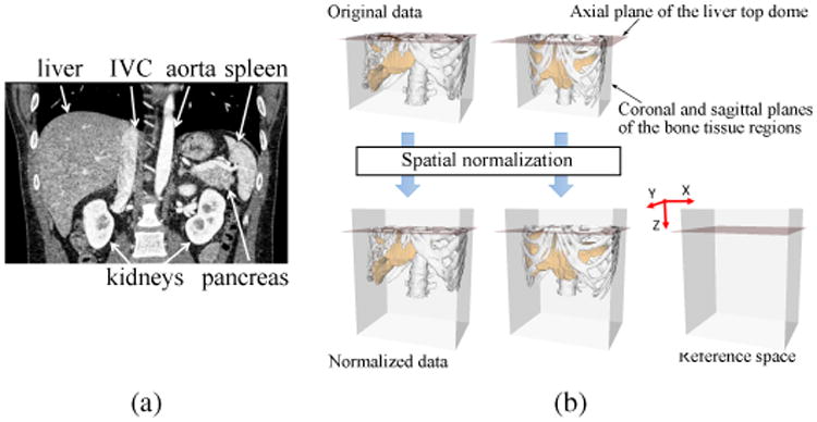
Spatial normalization. (a) Coronal view of typical our CT data. (b) Definition of the abdominal normalized space. In spatial normalization, the xyz-translation and xy-scaling are adjusted so that the reference planes are aligned among all the CT data. The z-scaling is not performed because stable image features were not available for the z-scale determination. In addition, strong correlation was not found between the xy- and z-scaling at least for the liver shape. Although only sagittal planes are shown in the figures, coronal planes are similarly defined. See Appendix A for an automated method for the spatial normalization.
Let I(x) be the target CT image data after spatial normalization. That is, I(x) denotes the CT value (intensity) at 3D coordinates x. Let k be organ index, and Lk(x) be the segmented label image of organ k, where Lk(x) = l ∈ {0, 1}, in which l = 1 denotes object, l = 0 background. A set of shape–location and intensity priors for organ k are given by
| (1) |
where Pk(x) denotes a PA, sk(b) = s̄k + Φkb a SSM, and Hk(I) = {HOk(I), HBk(I)} an IM for organ k, in which b = (b1 b2 ⋯ bm)t is the shape parameter vector, s̄k and Φk the average shape and the m eigenvectors of the SSM of organ k, respectively, and HOk(I) and HBk(I) the normalized histograms of organ k and its background regions, respectively. HOk(I) and HBk(I) are normalized so that their integral is 1. Given Ak, segmentation of organ k from I(x) is denoted by
| (2) |
where S eg(·) denotes the segmentation operation.
The single-organ segmentation method consists of three sub-modules as follows:
PA-based maximum a posteriori (MAP) segmentation
SSM-based refinement
Graph-cut refinement
Figure 2 shows the block diagram of the single-organ segmentation method. Details of the above three submodules of single organ segmentation are described in Appendix B.
Figure 2.
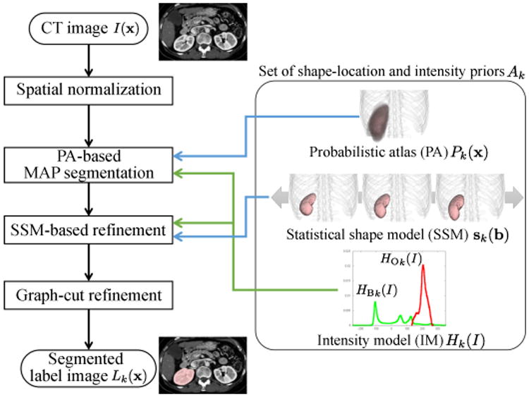
Block diagram of single-organ segmentation method. As an example, the segmentation target is R-kidney here. This is utilized as a basic module for multi-organ segmentation, where (conventional) PA and SSM will be replaced by prediction-based conditional ones described in Section 2.2. Three methods for constructing intensity models will be considered in Section 2.3.
2.2. Prediction-based shape–location priors
2.2.1. Statistical shape prediction using PLS regression (PLSR)
Let s0 and sk (k = 1,…, n) be the surface shape vectors of the target organ and its predictor organs, respectively, which are represented by the concatenation of the 3D coordinates on the surface of the organ, where n is the number of organs used to predict a target (For example, the target organ is the pancreas while the predictor organs are the liver and spleen as explained in Figs. 3 and 4.). Given the shape vectors of n + 1 organs of N cases (subjects) {ski} (k = 0,…, n, i = 1,…, N) as training datasets, the regression model predicting the shape vector of the target organ from n predictor organs is calculated using PLSR (Geladi and Kowalski, 1986). Unlike other standard least squares methods, PLSR works even when the predictor dataset is highly collinear. Yang et al. (2008) successfully applied PLSR to shape prediction of anatomical structures. Let be the predictor vector of case i. Given training datasets Tp = (s̃1 s̃2 ⋯ s̃N)t and Tt = (s01 s02 ⋯ s0N)t, the PLSR model to predict target vector ŝ0 from predictor vector s̃ is given by
Figure 3.
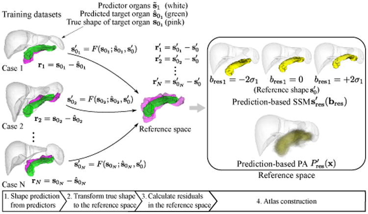
Construction of prediction-based shape–location priors in reference space. Green shapes in training dataset and reference space indicate the predicted and reference shapes of the target organ (which is the pancreas in this figure), respectively. Pink shapes in training dataset and reference space indicate the true shapes and transformed true shapes of the target organ, respectively. White shapes indicate the predictor organs, which are the liver and spleen in this case. After predicting the target organ shape from predictor organs, true shapes are transformed to reference space. Then SSM and PA of the residuals are constructed in the reference space.
Figure 4.
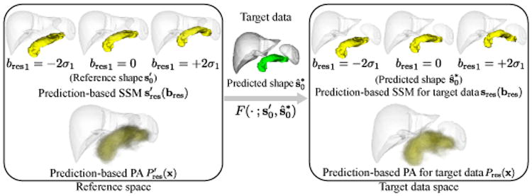
Generating prediction-based shape–location priors for segmentation of target data. Given segmented predictor organs of the target data, the target organ shape ŝ0t is predicted. The mapping defined by the deformation field from reference shape to predicted shape, , is applied to the prediction-based SSM and PA in the reference space to obtain those in the target data space.
| (3) |
where s̃ is the predictor vector for a data not included in the training dataset. The details of the training of the prediction model PLS R(s̃; Tp, Tt) are described in Appendix C.
2.2.2. Construction of prediction-based shape–location priors
Let (k = 1,…,n) be the segmented shape vectors of n predictor organs and be the predictor vector, where the shape vector with superscript *, e.g. , denotes the automatically segmented shape vector for target data, while the shape vector without superscript *, e.g. sk, denotes the shape vector for manual tracing of the training dataset. is obtained by fitting the SSM of organ k to the segmentation result Lk(x). The prediction function is defined as
| (4) |
where
| (5) |
and r denotes the residual after the prediction which is the difference between predicted and true shapes. In this work, the residual r is represented using PA and SSM as prediction-based shape–location priors.
Figure 3 shows the construction process for the prediction-based shape–location priors. To obtain PA and SSM of r, we perform the shape prediction of the target organ within the training dataset in a leave-one-out manner, and use the average shape of Tt as the reference shape . Let ri = s0i − ŝ0i be the residual of case i in the prediction whose model is trained without data of case i, where s0i and ŝ0i are the true and predicted target organs of case i, respectively. The dense 3D deformation field from the original space to the reference space is determined by thin-plate spline interpolation using correspondences from ŝ0i to . These correspondences are known because they are represented by the same SSM. The true shape s0i in the original space is mapped to the reference space using the determined deformation field, and the mapped version of the true shape s0i is given by , where F(· ; a, b) denotes the mapping function defined by the deformation field determined by thin-plate spline interpolation from shape vectors a to b. The difference between predicted and true shapes in the original space can be represented in the reference space by this mapping.
Now, the residuals in the reference space are given by . SSM and PA of are constructed in the reference space. Let be a label image which is voxelized from the surface of shape vector . PA and SSM in the reference space are given by
| (6) |
| (7) |
where Φres denotes the principal components of the residual and bres their coefficients. Because is the label image of the predicted organ shape of each case and regarded as the composition of reference shape and residual , smaller residuals result in less ambiguous PA.
Figure 4 shows the generation process of subject-specific shape–location priors. When prediction-based priors are utilized for segmentation of a target data, their subject-specific versions are obtained as follows. By using the mapping through the deformation field from the reference space to the target data space, , the prediction-based priors in the target data space are given by
| (8) |
| (9) |
where F−1(·) indicates the inverse mapping of F(·). In Eq. (8), it is necessary to use the inverse mapping F−1(·) in order to obtain the coordinates in the reference space corresponding to x since x is the coordinates in the target data space.
Given the set of segmented shape vectors of the predictor organs, , the set of shape–location and intensity priors is given by
| (10) |
Segmentation is performed using the method described in Section 2.1 by replacing Ak with Ak(S*) in Eq. (2). That is, the generated subject-specific versions of the prediction-based PA and SSM are utilized for segmentation by replacing the conventional PA and SSM in Fig. 2 with them.
Figure 5 shows prediction-based PAs for the R-kidney, GB, and pancreas (in comparison with conventional ones), which demonstrates that the prediction-based PA varies depending on the shapes of predictor organs. In Fig. 5, the predictor organs of the R-kidney, the GB, and the pancreas are the liver, the liver, and the liver and spleen, respectively. These relationships can be represented using directed graphs. The organs are represented as nodes of a graph, and predictor-target relations as directed edges. Using this graph representation, Figs. 5(a), (b), and (c) are represented as Figs. 5(d), (e), and (f), respectively. In Section 2.4, we formulate this graph representation as OCG.
Figure 5.

Conventional and proposed prediction-based PAs. (a) R-kidney. (b) GB. (c) Pancreas. Left: Conventional PA. Right: Proposed prediction-based PA using the predictor organs (the liver for R-kidney and GB, and the liver & spleen for the pancreas). The variations of the prediction-based PA due to the deformations of the predictor organs are shown. (d), (e), and (f) Graph representations of (a), (b), and (c), respectively.
2.3. Estimating intensity model (IM) from untraced CT data
Segmentation is performed using the methods described in Section 2.1 by replacing HOk(I) and HBk(I) with the IMs described below. Three types of IMs are constructed as follows:
Target-data specific IM (TD-IM): Only one CT data, which is the segmentation target, is used. Preparation of any training data is unnecessary for intensity modeling. Therefore, this model is immediately adaptable to any unknown imaging condition (IC) as far as shape–location priors are available.
Imaging-condition specific IM from untraced CT data (unsupervised IC-IM): In addition to the target CT data to be segmented, a sufficient number of CT data from different patients acquired by the same IC (protocol) as the target data are used. Laborious manual tracings are not required for intensity modeling of different ICs, and just original CT data are required for training. These training data are easy to collect from clinical image repositories.
Imaging-condition specific IM from traced CT data (supervised IC-IM): A sufficient number of CT data, which were acquired using the same IC as the target data and associated with manual tracings of the target organ, are used (Linguraru et al., 2012b; Okada et al., 2012a). This model requires a sufficient number of manual tracings for each different IC.
2.3.1. TD-IM
TD-IM is constructed as follows. Let I0(x) be the target CT data and P(x) the PA. Figure 6 shows the construction processes for TD-IM. First, P(x) is binarized using the threshold value determined by the 1st percentile in the probability distribution of P(x). Let the binarized region be RPA(x), which is used as the initial region for intensity modeling. Because the initial region RPA(x) should be highly likely to belong to the target organ region, only the 1st percentile is used. The initial histogram HO0 is obtained from the intensity distribution of I0(x) within RPA(x), and HO0 is normalized so that its integral is 1. The refined region R(x) is then obtained by applying the MAP segmentation (described in Appendix B.1) to I0(x) using P(x), HO0, and HB0, where HB0 is the histogram for background, which is obtained from I0(x) within the region where the probability value of P(x) is less than 5%. The processes obtaining HO0 with R(x) and updating R(x) by MAP segmentation are iterated three times. Finally, TD-IM HO and HB are obtained as HO0 and HB0, respectively, after the iterations. The prediction-based PA can be used as P(x) if the pre-segmented organ regions are available.
Figure 6.
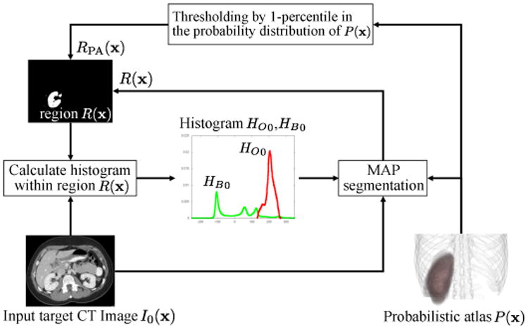
Process of construction of target-data specific intensity model (TD-IM). TD-IM HO and HB are obtained by iterating the processes obtaining HO0 with R(x) and updating R(x) by MAP segmentation.
2.3.2. IC specific IM from untraced CT data (unsupervised IC-IM)
The unsupervised IC-IM is constructed as follows. Let I = {Ii}(i = 1,…, N) be N additional CT data from different patients acquired using the same IC as I0 with the assumption that manual tracings are unavailable for these CT data. TD-IM is obtained for each Ii(i = 0,1,…, N). Note that segmentation target data I0 is also involved in intensity modeling. Let HO = {HOi} and HB = {HBi} (i = 0,1, …, N) be the histograms for object and background, respectively. Unsupervised IC-IM H̄ = {H̄O, H̄B} are calculated as
| (11) |
| (12) |
where ZO and ZB are normalization factors so that integral is 1.
2.3.3. IC specific IM from traced CT data (supervised IC-IM)
The supervised IC-IM is a conventional IM based on manual tracings in the training data, and is constructed as follows. Given I = {Ii}, which are acquired using the same IC as I0, with their corresponding manual tracings L = {Li} (i = 1,…, N), the supervised IC-IM H̄L = {H̄O,L, H̄B,L} are given by
| (13) |
| (14) |
where H(I; Ii, Li) is the histograms of intensity distributions of Ii within Li and the complement of Li.
2.4. Multi-organ segmentation based on organ correlation graph (OCG)
In this section, we formulate the predictor-target relations among the abdominal organs described in Section 2.2, by which the prediction-based priors are constructed, as the OCG. The OCG is defined as a set of nodes and directed edges. Each node corresponds to an organ and each directed edge denotes the correlation between one organ and another. Examples of simple OCGs are shown in Figs. 5(d), (e), and (f). The basic assumption is that automated segmentation of organs with out-edges in the OCG is sufficiently stable for use of these organs as predictors, while the organs with in-edges are effectively predicted by organs with out-edges. In the following, we describe how the predictor-target relations among the eight organs which we consider, that is, the liver, spleen, L-kidney, R-kidney, GB, aorta, IVC, and pancreas, are embedded into one OCG and how the conditional segmentation procedures are derived from the OCG.
Among the eight organs, segmentation of the liver has been studied intensively, and is now sufficiently accurate and stable by itself (Bagci et al., 2012; Linguraru et al., 2012b; Wolz et al., 2013; Montillo et al., 2011; Suzuki et al., 2012a; Seifert et al., 2009; Ling et al, 2008; Kohlberger et al., 2009; Okada et al., 2008; Zhang et al, 2010; Kainmüller et al., 2007; Massoptier and Casciaro, 2007; Shimizu et al, 2007; Lamecker et al., 2004; Park et al, 2003; Camara et al., 2004; Glocker et al., 2012). Segmentation of the spleen and kidneys has also been studied by a sufficient number of works, which showed sufficient accuracy (Bagci et al., 2012; Linguraru et al., 2012b; Wolz et al., 2013; Suzuki et al., 2012a; Montillo et al, 2011; Seifert et al., 2009; Shimizu et al, 2007; Glocker et al, 2012; Cuingnet et al., 2012; Freiman et al, 2010; Khalifa et al., 2011; Chen et al., 2012; Park et al, 2003; Camara et al, 2004). Finally, segmentation of other organs has not been well-established or shown to be accurate enough (Hammon et al., 2013; Wolz et al, 2013; Suzuki et al., 2012a; Shimizu et al., 2010, 2007; Zhou et al., 2010; Yoshida et al., 2011; Kurkure et al., 2008; Duquette et al., 2012; Montillo et al., 2011; Sanchez-Castro et al, 2010). Based on the above observations, we classify the eight organs or nodes into the following three types:
Type 1: Only out-edges are defined. Because no in-edges are defined, the segmentation of this type of organs is performed unconditionally. The liver is assigned to this type. The liver is particularly large compared with other abdominal organs. Especially in the prediction of small organs, only the local shape of the liver may be closely related to them. Thus, for effective prediction, we divide the liver surface into four sub-shapes. Figure 7 shows the four sub-shapes of the average liver, and three different patient liver shapes. The division method based on canonical correlation analysis developed by Yokota et al. (2013) was used for dividing the liver surface. The division method is detailed in Appendix D. The set of (sub-)organs of Type 1 is denoted as V1 = {liver1, liver2, liver3, liver4}.
Type 2: Both in- and out-edges are defined. Analysis of these organs is performed under the condition that the segmentation is completed for at least one node connected by an in-edge. In addition, the organ can be a predictor for nodes connected by out-edges. The set of organs of Type 2 is denoted as V2 = {spleen, R-kidney, L-kidney}.
Type 3: Only in-edges are defined. Segmentation of these organs is performed conditionally like for V2. This type cannot be a predictor. The set of organs of Type 3 is denoted as V3 = {pancreas, GB, aorta, IVC}.
Figure 7.

Four sub-shapes of the liver shape. (a) Average shape. (b) Three different patient liver shapes. Red, green, blue, and yellow sub-shapes are liver1, liver2, liver3, and liver4, respectively.
Table 3 summarizes the organ classification described above.
Table 3.
Organ classification. Type 1 organs are segmented unconditionally and are always predictor organs. Type 2 organs are segmented conditionally and can be predictor organs. Type 3 organs are segmented conditionally and cannot be predictor organs.
| Type | Set of organs | Role |
|---|---|---|
| Type 1 | V1 = {liver1, liver2, liver3, liver4} | predictor |
| Type 2 | V2 = {spleen, R-kidney, L-kidney} | predictor and target |
| Type 3 | V3 = {pancreas, GB, aorta, IVC} | target |
Given the constraints on the above three types of nodes, edge connections representing organ correlations are automatically defined based on shape predictability by PLSR described in Section 2.2.1. Let Vp = V1 ∪ V2 be a set of nodes for predictors, Vt = V2 ∪ V3 be a set of nodes for target organs, and Vp(vt) be the set of predictors of target organ vt ∈ Vt. Vp(vt) is determined by selecting the set of predictors which minimize the prediction error for vt among all possible combinations of nodes in Vp. Let be all possible combinations of nodes in Vp, where denotes the set of all k-combinations in Vp. Let TV and Tvt be the training data of organ shapes of V ∈ Vall and vt ∈ V t, respectively, and ε(V; vt) be the prediction error of vt using the prediction model PLS R(s̃; TV, Tvt) (see Appendix C). Then the set of predictor nodes Vp(vt) for vt is defined as
| (15) |
The OCG is defined as OCG =< V, E > with
| (16) |
| (17) |
where
| (18) |
denotes a set of directed edges toward vt. The relations between each target and its predictors in PLSR that minimizes the prediction error are associated with the edges of OCG. Figure 8(a) shows the OCG of the eight organs constructed from our training data.
Figure 8.
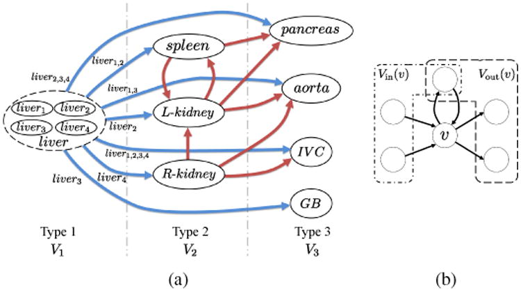
Organ correlation graph (OCG). (a) OCG constructed from eight abdominal organs. Blue and red edges indicate the edges from nodes of Types 1 and 2, respectively. For simplicity, the multiple edges from the sub-shapes of the liver to a target organ are indicated by one edge from the liver to it and the identifiers of sub-shapes are indicated by the labels on the edges. In the graph, a node having in-edges is predicted from nodes having out-edges. (b) Examples of Vout(v) and Vin(v). As shown in this figure, some nodes can be included in both Vout(v) and Vin(v).
The synchronized processes of multi-stage updating in multi-organ segmentation based on OCG are formulated in Algorithm 1. Let v be a node (that is, an organ) to be segmented, Vout(v) be a set of nodes with the edge from v, and Vin(v) be a set of nodes with the edge toward v. Figure 8(b) shows examples of Vout(v) and Vin(v). Here, we assume that one or more nodes in Vin(v) have already been segmented at the current stage. Segmentation of node v is performed using prediction-based shape–location priors constructed from segmented nodes in Vin(v). Note that the segmentation result of a target organ is not directly used as the initial region in its segmentation processes at the next stage. It is used only for updating prediction-based priors at the next stage. After segmentation of v, all nodes in Vout(v) become ready for segmentation at the next stage. Let j be the index of the segmentation stage. Node v is ready for segmentation at stage j after at least one node in Vin(v) has been segmented during stage j − 1. If Vin(v) is empty, e.g. V1 (the liver in this study) does not have in-edges, segmentation of v is completed using conventional shape–location priors without predictor organs. That is, segmentation of organ v in V1 can be performed at the initial stage (Stage 0) of the segmentation processes. Figure 9 shows the states of OCG at different stages in multi-organ segmentation processes. Let jmax be the maximum number of stages of the segmentation processes, be a set of nodes ready for segmentation at Stage j, and Vsegmented be a set of segmented nodes. Multi-stage updating of the segmentation processes is repeated at least until is unchanged. Figure 10 shows examples of prediction-based PAs at different stages in multi-organ segmentation processes for three cases.
Figure 9.
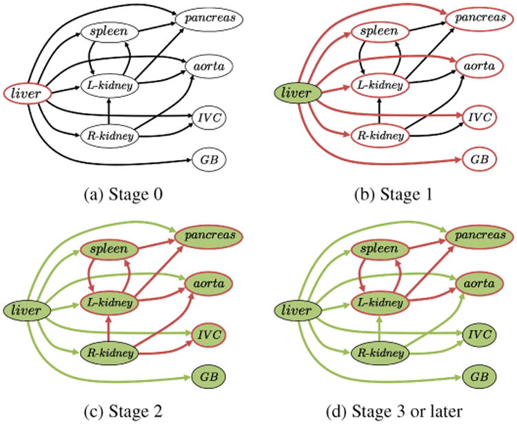
Processes of multi-stage updating in multi-organ segmentation based on OCG. Red contoured nodes indicate those to be segmented. Green-colored nodes indicate those that have already been segmented. (a) Stage 0. The liver (only one organ in V1) is firstly segmented. (b) Stage 1. The organs connected from the sub-shapes of the liver are segmented. (c) Stage 2. The organs connected from those segmented at the previous stage are segmented. Note that the R-kidney and GB are not segmented at this stage because the segmentation results of predictors (only the liver in this case) do not change. (d) Stage 3 or later. Further segmentations are performed using updated results of the predictors.
Figure 10.
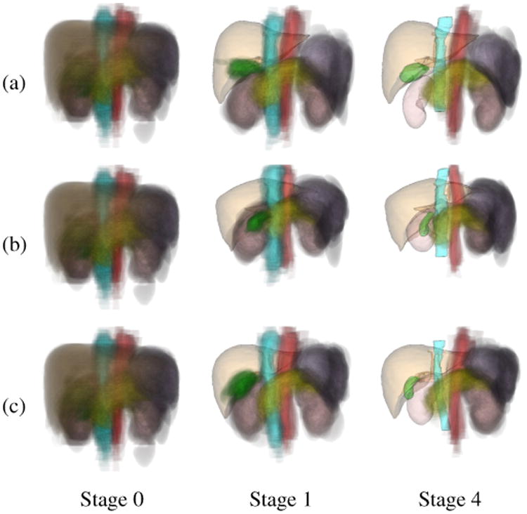
Examples of prediction-based PAs at different stages of multi-organ segmentation. (a) Case 1. (b) Case 2. (c) Case 3. Left: Conventional PA of eight organs (Stage 0). Middle: Prediction-based PAs using the segmented liver (Stage 1). Right: Prediction-based PAs using the segmented liver, spleen, and kidneys (Stage 4). Orange indicates the liver, purple the spleen, pink the kidneys, yellow the pancreas, green the GB, red the aorta, and cyan the IVC. PAs are illustrated by cloud-like semi-transparent volume rendering. The segmented organ shapes are represented by semi-transparent surface rendering. At Stage 4, segmentation of R-kidney, gallbladder, and IVC (in addition to the liver) stops updating, and thus their segmented surfaces are shown instead of PAs.
|
| ||
| Algorithm 1 Multi-organ segmentation based on OCG | ||
|
| ||
| Input: Target image I(x), OCG =< V, E >, number of stages jmax | ||
| Output: Label images of each organ {Lv(x) | v ∈ V} | ||
| 1: | Vsegmented ← ∅ | |
| 2: |
|
|
| 3: | for j = 0 to jmax do | |
| 4: | for all do | |
| 5: | ||
| 6: | Lv(x) = S eg(I(x); A(S*)) | |
| 7: | ← shape vector calculated by fitting SSM to Lv(x) | |
| 8: | end for | |
| 9: | ||
| 10: | ||
| 11: | end for | |
|
| ||
3. Experimental Results
3.1. Dataset
We tested the proposed methods using 134 abdominal CT data from 86 patients (cases) obtained under six different ICs at two hospitals: Osaka University Hospital, Japan (OUH) and National Institutes of Health, USA (NIH). Table 4 shows the details of six ICs. Figure 11 shows examples of CT data of six ICs. CT data obtained at OUH were two-phase CT data of 49 cases. The contrast phases used in image acquisition were early and late arterial phases (which were Datasets A and B, respectively). Data for 10 cases (Datasets A-1 and B-1) were acquired using a 4-slice Light Speed QX/i (GE Healthcare) scanner while data for the other 39 cases (Datasets A-2 and B-2) were acquired using a 64-slice Light Speed VCT (GE Healthcare) scanner, among which only the late arterial phase was available for one case. CT data obtained at NIH included 25 cases from the portal venous phase (Dataset C) and 12 cases from the non-contrast CT data (Dataset D). These data were acquired using a 4-slice HighSpeed QX/I (GE Healthcare), an 8-slice Light-Speed Ultra (GE Healthcare), a 64-slice Brilliance 64 (Philips Healthcare), a 16-slice Mx8000 IDT 16 (Philips Healthcare), and a dual source 256-slice Definition Flash (Siemens Healthcare). Eight organs (the liver, spleen, L-kidney, R-kidney, GB, aorta, IVC, and pancreas) were manually segmented from all data under the supervision of experienced radiologists.
Table 4.
Details of CT scans used in experiments.
| Dataset | Institution | Phase | # of cases | Slice thickness [mm] | |
|---|---|---|---|---|---|
| A | A-1 | Osaka Univ. Hospital (OUH) | Early arterial phase | 10 | 2.5 |
| A-2 | 38* | 0.625 | |||
| B | B-1 | Late arterial phase | 10 | 2.5 | |
| B-2 | 39* | 0.625 | |||
| C | NIH | Portal venous phase | 25 | 0.68 – 1.25 | |
| D | Non-contrast | 12 | 1.0 | ||
: Only late arterial phase was available in one case.
Figure 11.
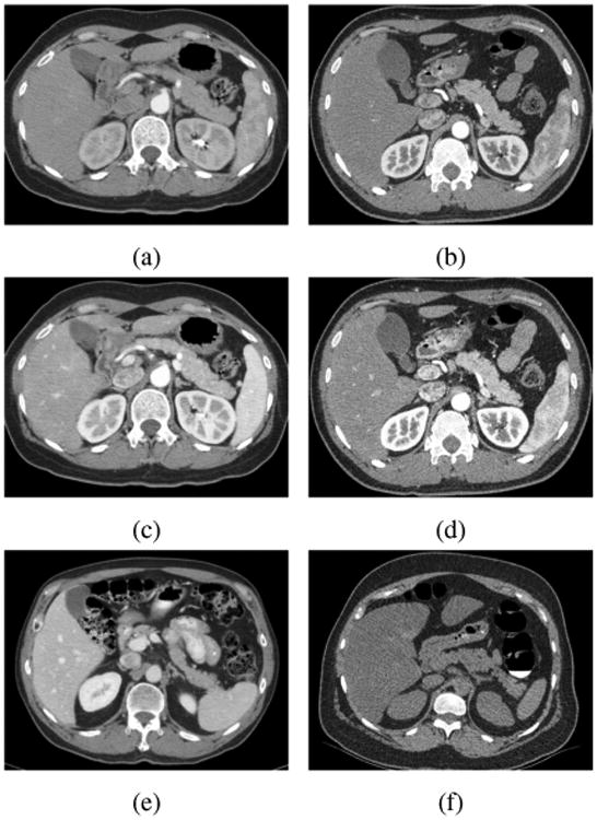
Examples of cross-sectional CT images of our data. See Table 4 for the descriptions of each IC. (a) A-1, (b) A-2, (c) B-1 (d) B-2, (e) C, and (f) D.
Because the liver was segmented using only the conventional single-organ segmentation method, the descriptions of results focuses on the other seven organs.
3.2. Experimental method
Two-fold cross validation was performed. The datasets from each IC was randomly separated into two datasets, that is, training and test datasets. Shape–location priors were constructed using the training dataset from all ICs. Note the unsupervised IC-IM was estimated using the test dataset from each IC, and thus was not based on any intensity information combined with manual tracings.
Segmentation using conventional shape–location priors and/or supervised IC-IM were also performed for comparison purpose. We did not use the training dataset but used the test dataset for constructing the supervised IC-IM, which was also used for the unsupervised IC-IM, because the difference in performance due to the method of IM construction will not be properly evaluated if the different datasets were used for constructing IM. Optimization of segmentation parameters was performed using only the training dataset. Note that the test dataset was totally separated from parameter optimization. The details of the parameter optimization are described in the next sub-section. Initially, segmentation of the liver was performed using conventional shape–location priors and TD-IM (Okada et al., 2008). Subsequent segmentations of other organs were performed using three IMs (TD-IM, unsupervised IC-IM, and supervised IC-IM). The maximum number of stages of multi-organ segmentation was jmax = 4. Two-fold cross validation was performed for five different patterns of two-fold separations of the dataset, which were randomly generated, and the results were averaged. Dice Coefficient (DC) (Dice, 1945), Jaccard Index (JI) (Jaccard, 1901), and Average Symmetric Surface Distance (ASD) (Heimann et al., 2009) were used for quantitative evaluation.
3.3. Parameter optimization
Parameter optimization was performed using leave-one-out cross validation only within a subset of the training dataset for each organ. In order to avoid over-tuning in the parameter optimization, we selected the training data so as to exclude CT data of the same IC as the test data. Because CT data acquired from OUH did not include the same ICs as those from NIH, and vice versa, parameter optimization was performed for one institution using training dataset from the other institution. Segmentation using conventional shape–location priors (described in Section 2.1) was performed, and the set of parameter values with which the best segmentation accuracy achieved were selected as follows (Details of the algorithms including these parameters are described in Appendix B.):
Radius ρ of the structuring element in opening and closing at the final step of PA-based segmentation: The optimal value of ρ was selected so as to maximize the PA-based segmentation accuracy.
Weight parameter λ in SSM-based refinement: The optimal value λ was selected so as to maximize the SSM-based refinement accuracy, given PA-based segmentation results using the optimal ρ.
Threshold values pO and pB to determine regions of hard constraint in graph-cut refinement: Optimal values of pO and pB were selected so as to maximize the graph-cut refinement accuracy, given the segmentation results obtained using PA-based segmentation with the optimal ρ followed by SSM-based refinement with the optimal λ.
We used Jaccard index (JI) as the segmentation accuracy measure in the above procedures.
During cross-validations for parameter optimization, the most frequently selected values for radius ρ in PA-based segmentation, weight parameter λ in SSM-based refinement, values pO and pB in graph-cut refinement were ρ = 1, λ = 0.5, pO = 0.1, and pB = 2, respectively.
3.4. Results
Figure 12 summarizes the results of comparisons of segmentation accuracy between methods using the proposed prediction-based and conventional shape–location priors. In these comparisons, the unsupervised IC-IM was used for intensity modeling. As shown in Fig. 12, significant accuracy improvement by using the proposed priors was observed for all seven organs in comparison with the conventional priors. Significance was determined using paired T-test with significance levels of 0.01 and 0.05. For most organs and evaluation measures, significant improvements in accuracy with a significant level of 0.01 were observed, excepting that the R-kidney in DC and the spleen in ASD showed a significance level of 0.05.
Figure 12.
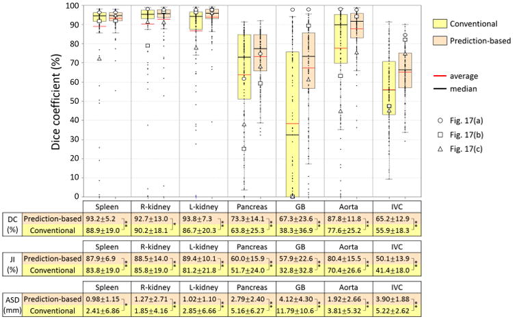
Summary of accuracy evaluation for proposed prediction-based and conventional shape–location priors when unsupervised IC-IM was used for intensity model. Dice coefficients (DCs) of 134 CT data using prediction-based and conventional shape–location priors for each of seven organs were plotted. The averages of DC, Jaccard index (JI), and average symmetric surface distance (ASD) as well as statistical significance are also shown in a table format. In the table, * and ** indicate that significant accuracy improvement with significance levels of 0.05 and 0.01 was observed, respectively. DCs of three cases indicated in Figs. 17(a), (b), and (c) are plotted by ○,□, and Δ, respectively.
Figure 13 shows the accuracy improvement of each segmentation submodule, which corresponds to each block of Fig. 2. The shape-location and intensity priors were the same as used in the proposed method in Fig. 12. The average shape of the prediction-based SSM (conventional SSM only for the liver) was used to evaluate the accuracy of the spatial normalization. The segmentation accuracy was monotonically increased as subsequent submodules were combined. Significant accuracy improvements were observed among all submodules for all organs (p < 0.01).
Figure 13.
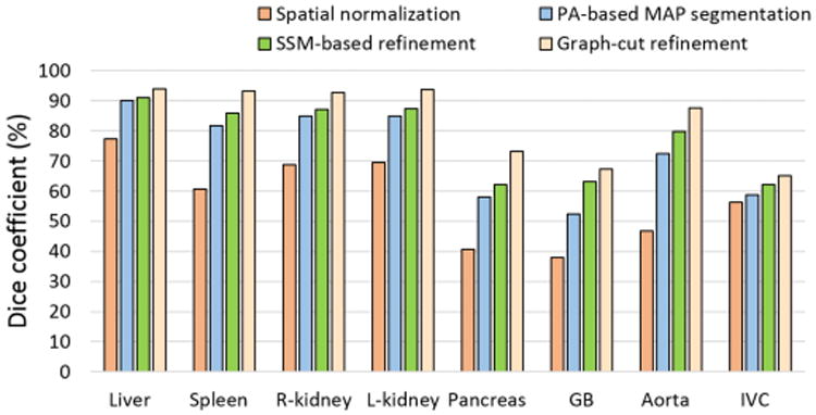
Accuracy improvement of each segmentation submodule corresponding to each block in Fig. 2. The same shape-location and intensity priors were used as the proposed method in Fig. 12. Statistical significance was observed among all submodules for all organs (p < 0.01).
Figure 14 shows the effects of the multi-stage updating in the proposed multi-organ segmentation based on OCG, where average DC at each stage was plotted for each organ. Our multistage updating method does not guarantee the convergence. To confirm the behavior of multi-stage updating, we performed experiments up to Stage 8. Because similar results were obtained in Stage 4 or later, the results up to Stage 4 are shown in Fig. 14. The accuracies at Stage 3 or later (using all available predictor organs) were significantly improved in comparison with Stage 1 (using only the liver as the predictor organ) for the L-kidney (p < 0.05). The accuracies at Stage 2 or later were significantly improved in comparison with Stage 1 for the pancreas (p < 0.05) and aorta (p < 0.01). For the IVC, significant improvement was observed between Stage 1 and Stage 2 (p < 0.05). For the spleen, however, no significant improvement in accuracy was observed (the range of p-value was from 0.084 to 0.337 among Stage 1 and later stages). For the R-kidney and GB, segmentation accuracy was not changed through Stages 1 to 8 because only the liver was used as the predictor organ. The accuracy variations from Stages 3 to 8 were calculated as the difference of the maximum and minimum DCs. The maximum variation was 0.32%, which was observed in L-kidney.
Figure 14.
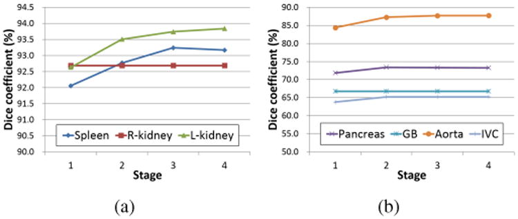
Effects of multi-stage updating in proposed multi-organ segmentation based on OCG. Average DC of 134 CT data at each stage is plotted for each organ. (a) Plots for the spleen, R-kidney, and L-kidney. (b) Plots for the pancreas, GB, aorta, and IVC. Only the liver was used as the predictor at Stage 1. The spleen, R-kidney, and L-kidney were used as the predictors in addition to the liver at Stages 2 to 4.
The proposed method assumes that the liver is initially segmented. Hence, failure of liver segmentation may affect subsequent predictions and segmentation of other organs. In order to examine the effects of segmentation accuracy of the liver on other organs, the datasets used in the experiments were divided into two groups based on the accuracy of liver segmentation, that is, those below and above the lower quartile of DC of liver segmentation. Table 5 shows average DCs of the seven organs for the two groups. Although significant difference was not observed in all seven organs between the two groups, the average DCs of R-kidney, GB, and IVC, which are adjacent to the liver, decreased by 11.0, 19.3, and 9.7 percentage points, respectively, in the group below the lower quartile. For other organs, the accuracy decrease was 0 to 5 percentage points.
Table 5.
Average DCs of two groups of datasets whose accuracies of liver segmentation were below and above the lower quartile (LQ).
| Liver segmentation accuracy | Spleen | R-kidney | L-kidney | Pancreas | GB | Aorta | IVC | |
|---|---|---|---|---|---|---|---|---|
| DC [%] | Below the LQ (Low accuracy) | 91.8 | 84.5 | 91.9 | 69.2 | 52.9 | 87.7 | 58.0 |
| Above the LQ (Medium and high accuracy) | 93.7 | 95.5 | 94.5 | 74.7 | 72.2 | 87.8 | 67.7 |
In order to evaluate the accuracy of the unsupervised IC-IM estimation rather than final segmentation accuracy, similarities between unsupervised and supervised IC-IMs were calculated using normalized cross correlation (NCC). Figure 15 shows average NCCs of the six ICs for each organ. The average NCCs were improved and greater than 0.9 for all organs except for the GB by using the prediction-based PA, while the improvement was prominent especially in the GB.
Figure 15.
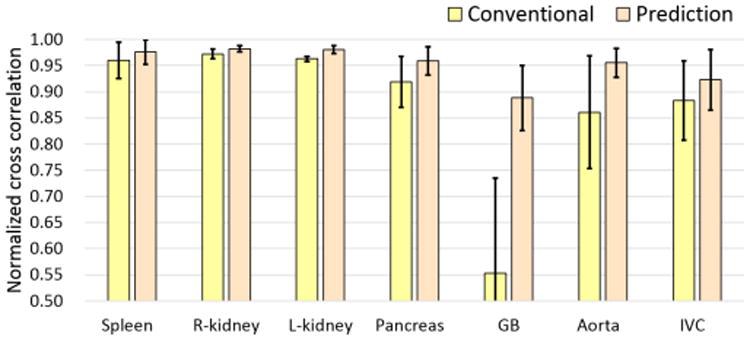
Similarity between supervised and unsupervised IC-IMs. Normalized cross correlations (NCCs) between supervised IC-IM and unsupervised IC-IM using conventional (yellow bar) and prediction-based PAs (orange bar) were shown. NCCs of the six imaging conditions were averaged.
Figure 16 summarizes segmentation accuracies for the three IMs using the proposed prediction-based shape–location priors. We first focus on the results in DC in this paragraph. The average DC of the liver, in which only TD-IM was used, was 94.1%. Average DCs of the spleen, R-kidney, and L-kidney were more than 90% for all three IMs. For the spleen and R-kidney, statistical significance was not observed among three IMs, although the standard deviation (SD) of TD-IM in the R-kidney was larger than the other two IMs. For the L-kidney, statistical significance was observed between TD-IM and supervised IC-IM (p < 0.05). Nevertheless, the decrease in accuracy was not obvious. The average DC of the pancreas was around 73% for all three IMs and statistical significance was not observed among them. However, the SD of TD-IM was slightly larger than other IMs. For the GB, the unsupervised IC-IM was significantly more accurate than TD-IM (p < 0.01). Furthermore, the supervised IC-IM was significantly more accurate than unsupervised IC-IM (p < 0.01). As shown in Fig. 15, the similarity of the estimated IMs between the supervised and unsupervised IC-IMs was lower in the GB than in other organs. Note that the GB is small and has large inter-subject location variability, which makes it difficult to ensure a sufficient amount of high probability area even in the prediction-based PA. For the aorta, TD-IM was significantly less accurate than unsupervised and supervised IC-IMs (p < 0.05 and p < 0.01, respectively), and the SD of TD-IM was larger than other IMs. However, statistical significance was not observed between unsupervised and supervised IC-IMs. For the IVC, statistical significance was not observed among three IMs.
Figure 16.
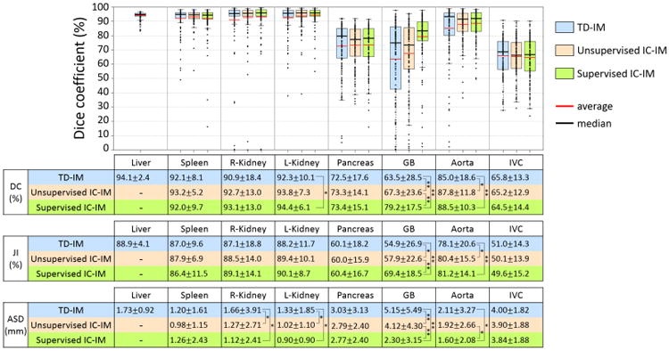
Summary of accuracy evaluation for three intensity models when the proposed prediction-based shape–location priors were utilized. DCs of 134 CT data using TD-IM, unsupervised IC-IM, and supervised IC-IM for each of eight organs were plotted. With respect to the liver, only the result using TD-IM is shown. Average DC, JI, and ASD values and statistical significance are also shown below the plots in a table format. In the table, * and ** indicate that significant accuracy improvement with significance levels of 0.05 and 0.01 was observed, respectively.
Similar results were obtained for evaluations by JI and ASD in Fig. 16. For the kidneys, accuracy in the TD-IM was significantly decreased in comparison with unsupervised and supervised IC-IMs in ASD (p < 0.05). However, statistical significance was not observed between unsupervised and supervised IC-IMs in ASD. For the aorta, supervised IC-IM was significantly more accurate than TD-IM and unsupervised IC-IM in ASD (p < 0.05). The results in Fig. 16 are summarized as follows. Unsupervised IC-IM was regarded as mostly comparable to supervised IC-IM excepting the GB. TD-IM was regarded as less accurate in the kidneys, aorta, and GB, but the accuracy decrease in the kidneys and aorta was not large.
Figure 17 shows illustrative three examples of segmentation results, which effectively demonstrate usefulness of the proposed methods. DC of each organ in these three cases is plotted in Fig. 12. In Fig. 17, the failed regions by the conventional prior are indicated by white arrows. In Fig. 17(a), the pancreas and IVC were better segmented by using the proposed prediction-based prior with different IMs. In the pancreas, the head of the pancreas was better segmented by using TD-IM than the other IMs (the improved part in TD-IM is shown by a black arrow). In Fig. 17(b), the pancreas, GB, aorta, and IVC were missed by the conventional prior while the prediction-based priors were effective. The segmentation result of the R-kidney was leaked into the liver by the conventional prior. In this case, the segmented liver region was leaked into the R-kidney, GB, and IVC. However, these organs were successfully segmented by using the prediction-based priors even when the leaked liver was used for the predictor organ. The regions of the liver leakage are indicated by white arrow heads in Fig. 17(b). In Fig. 17(c), the spleen, L-kidney, pancreas, GB, aorta, and IVC were better segmented by using the proposed prediction-based priors. For the GB, unsupervised IC-IM was worse than TD-IM and supervised IC-IM by the prediction-based prior (the failed part in unsupervised IC-IM is shown by a black arrow). In TD-IM, the pancreas was largely missed by the prediction-based prior while the other IMs were effective. As shown in Fig. 16, the SD of TD-IM for the pancreas was larger than other IMs. Figs. 17(a) and (c) indicate typical results which caused higher SD in TD-IM. In the illustrated three cases, the unsupervised IM combined with the prediction-based priors was superior or equivalent to the conventional priors for the segmentation of all seven organs.
Figure 17.
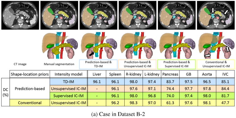
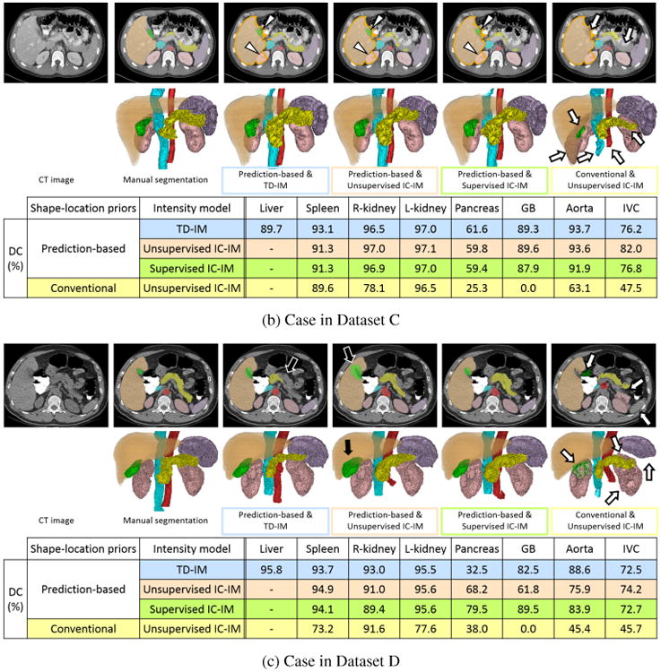
Illustrative segmentation results (a) Case in Dataset B-2 (arterial phase enhancement). (b) Case in Dataset C (portal venous phase enhancement). (c) Case in Dataset D (non-contrast). From the left to the right, input CT image, manual segmentation, and results using the proposed prediction-based shape–location priors & TD-IM (blue), the proposed prediction-based priors & unsupervised IC-IM (orange), the proposed priors & supervised IC-IM (green), and the conventional priors & unsupervised IC-IM (yellow). Upper Axial cross-section. Lower 3D rendering. Orange, purple, pink, yellow, green, red, and cyan volumes and regions indicate the liver, spleen, kidneys, pancreas, GB, aorta, and IVC, respectively. Dice coefficient (DC) of each segmented organ is also shown in a table format. In (b), orange contour indicates the contour of the liver region to show liver leakage. White arrows show the failed region by the conventional priors. Black arrows show the improved or failed regions by the prediction-based priors. Arrow heads show the regions of liver leakage.
4. Discussion
4.1. Summary of the proposed method
In this paper, we have described a general framework of multi-organ segmentation which effectively incorporates interrelations among multiple organs. The main contribution of this paper is that a method for modeling prediction-based conditional shape–location priors based on OCG is developed. In our framework, predictor organs, such as the liver, whose segmentation is sufficiently accurate by using conventional single-organ segmentation methods, are pre-segmented, and the remaining organs are hierarchically segmented using conditional shape–location priors. The prediction-based priors enabled sufficiently accurate estimation of intensity priors without using supervised intensity information. As shown in Fig. 12, the prediction-based priors were a significantly more effective way to estimate intensity priors and use them for segmentation without supervised intensity information in comparison to conventional priors.
As shown in Fig. 16, segmentation accuracy using TD-IM was slightly but significantly less accurate than supervised IC-IM in DC for the L-kidney and aorta. However, it became comparable by using unsupervised IC-IM for these organs. For the GB, the proposed IMs (TD-IM and unsupervised IC-IM) were significantly less accurate than supervised IC-IM, but unsupervised IC-IM was significantly more accurate than TD-IM. From these results that significant improvements were observed in GB (in DC, JI, and ASD), kidneys (in ASD), and aorta (in DC and JI) for unsupervised IC-IM compared to TD-IM, unsupervised IC-IM is considered to be a reasonable way of intensity modeling from a number of untraced CT data. In contrast, significant difference was not observed in the spleen, pancreas, and IVC among the three intensity models (in all of DC, JI, and ASD). Intensity variations are considered to be fairly large in these organs even within the same IC. Therefore, unsupervised and supervised IC-IMs were not so effective in these organs and TD-IM was comparable to them.
4.2. Effectiveness of the proposed method
As shown in Fig. 12, the largest improvement by using the proposed prediction-based priors was observed in the GB. Although the GB is a small organ and its inter-subject variation in location is relatively large, it is in contact with the liver. Therefore, the effect of the prediction of the GB from the segmented liver region was substantial. The improvement of unsupervised IC-IM estimation (Fig. 15) by the proposed prediction-based priors was particularly prominent for the GB.
As shown in Fig. 13, significant accuracy improvements were observed among all submodules for all organs. Among the submodules, improvements due to SSM-based refinement look relatively small (although statistical significance was observed). Therefore, additional experiments were conducted, in which graph-cut refinement was performed directly after PA-based MAP segmentation (without SSM-based refinement). The experimental results showed that the segmentation accuracy without SSM-based refinement was significantly decreased in comparison with that with SSM-based refinement (p < 0.01 for all organs). Therefore, all segmentation submodules were effective.
As shown in Table 5, the segmentation accuracy of the liver affected the accuracy of organs adjacent to the liver. In the experiments, the segmented liver region was often leaked into the GB and IVC. However, segmentation accuracy using prediction-based shape–location priors was improved in comparison with conventional ones even when this leakage occurred. In Fig. 17(b), the R-kidney, GB, and IVC were successfully segmented by using the proposed prediction-based priors although the segmented liver was leaked into them. Even when SSM fitting was performed to mis-segmented liver shape due to leakage in order to generate subject-specific versions of the prediction-based shape–location priors, sufficiently well-approximated liver shape for the predictor organ was recovered since SSM of the liver has specificity for the liver shape. Thus, appropriate predicted shapes of target organs and their prediction-based PAs were obtained (GB and IVC in Fig. 17(b)). Subsequent SSM-based and graph-cut refinements also contributed to the recovery from the failure in PA-based MAP segmentation (R-kidney in Fig. 17(b)). The behaviors of the proposed method as described above were observed in a few cases. The liver segmentation method used in this work was based on our previous work (Okada et al., 2008). It can be replaced by recently developed improved methods (Tomoshige et al., 2014; Umetsu et al., 2014), which showed good performance even for pathological and largely deformed livers. Therefore, improvement of liver segmentation accuracy would be expected.
Multi-stage updating in the proposed method was demonstrated to be useful (Fig. 14). Significant accuracy improvement in most of organs interrelated with multiple predictor organs was attained at Stage 4 (using multiple organs as the predictors) in comparison with Stage 1 (using only the liver), as described in the second paragraph of Section 3.4. Only in the spleen, significant improvement was not observed (although average accuracy increased). In addition, the accuracy decreased from Stage 3 to Stage 4 in the spleen. Our multi-stage updating method does not guarantee the convergence. Therefore, instability may be caused during the iteration. However, accuracy variations were within 0.32% in DC after Stage 3 and did not affect the results of significance test. Regarding the number of iterations, we consider that additional one or two iterations will be sufficient after the OCG reaches a steady state shown in Fig. 9(d). Accuracy variations during the iteration were mainly observed in the spleen and left kidney. Its potential cause is that these organs are the predictor and target organs each other (as shown in Fig. 9) and oscillation phenomena occurred in a few cases. When the OCG is constructed, the constraint to avoid such relations may be effective.
Among the eight organs, the GB was the organ for which supervised intensity information was significantly useful. However, if CT cholangiography data are given, in which the fluid in the GB is contrast-enhanced, our method may be easily adaptable while the conventional method requires a number of manual tracings to obtain supervised intensity information. With respect to the GB, its supervised IC-IM in non-contrast CT data will be generally applicable to most contrast-enhancement protocols and phases excepting CT cholangiography because the GB is usually unaffected by contrast media via blood vessels. Therefore, its supervised IC-IM will be worth being constructed through time-consuming efforts.
The experimental results show the effectiveness of the proposed unsupervised IC-IM although the number of input CT datasets for constructing IMs were about 20 at most. It is considered that collecting 20 or more CT datasets without manual tracing is easy in clinical practice. In the construction of the unsupervised IM, threshold value determined by the 1st percentile in the probability distribution of PA were used for binarization of PA. The number of voxels of the region determined by the 1st percentile were more than several thousand voxels by using prediction-based PA. It is considered that it was sufficient for the estimation of the initial histogram to be used for further MAP segmentation. Once core datasets with manual tracing are prepared for constructing shape–location priors, the proposed method can be applied to CT data of various ICs by collecting untraced CT datasets for the required IC. This feature is important for use in routine clinical practice. The number of training data for shape–location priors was 43 in our two-fold cross validation. It is expected that the segmentation accuracy will be improved by increasing the number of training data. Investigation of the effects of the number of training data on segmentation accuracy will be a future work.
4.3. Comparison with existing methods
We compare the segmentation accuracy of the proposed method with those reported in the previous literatures (Wolz et al., 2013; Linguraru et al., 2012b; Shimizu et al., 2010; Hammon et al., 2013) although the datasets used for evaluation were different. These previous works used supervised intensity information and were tested for one contrast-enhancement pattern of CT data. In the spleen and kidneys, the segmentation accuracy of the proposed method (92.7 to 93.8% in DC) was comparable to or slightly better than state-of-the-art methods using one phase of the contrast-enhanced CT data with supervised intensity information (92.0 to 92.5%, 150 cases (Wolz et al., 2013) and 90.9 to 92.9%, 28 cases (Linguraru et al., 2012b) in DC). In the pancreas, the proposed method (60.0% in JI) was also comparable to or slightly better than the methods using supervised intensity information (55.5%, 150 cases (Wolz et al., 2013), 57.9%, 20 cases (Shimizu et al., 2010), 61.2%, 40 cases (Hammon et al., 2013) in JI from contrast enhanced CT data) in spite that supervised intensity information was not used in the proposed methods. In the GB, the segmentation accuracy of the supervised IC-IM (69.4% in JI) was slightly better and that of unsupervised IC-IM (57.9% in JI) was slightly worse than the multi-organ segmentation method developed by Shimizu et al. (2007) (around 62% in JI), which utilized supervised intensity information inherent in non-contrast CT data and was tested only for 10 cases. Average JIs of the aorta (80.4%) and IVC (50.1%) in the proposed method with unsupervised IC-IM were comparable to or slightly better than the Shimizu's method (around 77% in aorta and 48% in IVC) (Shimizu et al., 2007). From the literatures, segmentation accuracy of the proposed method was summarized as mostly comparable to or slightly better than the state-of-the-art methods in spite that supervised intensity information was not used in it as well as mixture sets of contrast-enhanced and non-contrast CT data were tested.
From the methodological viewpoints, a particular feature which differentiates the proposed method from existing methods is explicit modeling and utilization of spatial interrelations among multiple organ shapes for prediction of the target organ regions. That is, the targets are predicted from neighboring organ regions. In contrast, the machine-learning approaches have typically used low-level image features such as anatomical landmarks for the prediction (Seifert et al., 2009; Montillo et al., 2011; Glocker et al., 2012; Criminisi et al., 2013). Its advantages would be that the salient features are automatically determined during learning processes. That is, the targets are predicted from low-level features. In the statistical and multi-atlas approaches, multi-resolution modeling of multiple organs has been mainly used for the prediction in order to gradually increase the prediction accuracy in a robust manner (Wolz et al., 2013; Iglesias et al., 2013; Cerrolaza et al., 2012, 2013; Bagci et al., 2012). That is, the targets are predicted from lower-resolution organ regions. Overall, each approach uses different context information for the prediction, which is suitable for its methodological characteristics. The proposed method provides a different source of the context information. Approaches to integrate different context information sources will be an important future work, one example of which is described next in Section 4.4.
4.4. Limitations and future work
In this method, spatial normalization is performed based on bone detection by simple thresholding and liver top detection by rough segmentation of the lung. Therefore, our current method for spatial normalization requires that these features and regions are imaged in the field of view (FOV) of input CT data, that is, the whole liver is included in the FOV. One possible method to overcome this limitation would be to use anatomical landmarks (Seifert et al., 2009; Hanaoka et al., 2011). We are currently considering a machine learning approach to perform spatial normalization based on detected anatomical landmarks.
As future work, it is desirable that the method is applicable to CT data with pathologies or missing organs. We are now extending the proposed method in the following points; (1) adding other abdominal organs, such as the gastrointestinal tract, to OCG (Hirayama et al., 2013), and (2) application to organ segmentation under pathological conditions (Fukuda et al., 2013). In addition, the proposed method obviously faces a problem when an organ is missing. A method for detecting missing organs, as proposed in Suzuki et al. (2012a), needs to be incorporated. Because specific patterns of organ shifts are statistically modeled after surgical removal of organs, as shown in Suzuki et al. (2012b), prediction-based shape–location priors would be constructed for each pattern of missing organs in order to reduce instability. With respect to intensity priors, our intensity modeling is currently based on intensity histograms of the organ and background regions. Incorporation of texture information inside the organ regions will improve the segmentation accuracy when neighboring organs have similar intensity histograms but different textures.
5. Conclusion
We have presented a general framework for multi-organ segmentation which is adaptable to various ICs without the need for supervised intensity information. In this paper, an OCG, which encodes the spatial correlations among organs, was introduced. By constructing and utilizing subject-specific shape– location priors based on shape prediction from pre-segmented organs, the segmentation accuracy of abdominal organs was largely improved. The initialization of organ locations and shapes becomes accurate enough to estimate IM in an unsupervised manner by using prediction-based shape–location priors. Average DCs of the liver, spleen, and kidneys were more than 92%. Average DCs of the pancreas, GB, and IVC were around 73%, 67%, and 65%, respectively. These results were comparable to state-of-the-art segmentation methods using supervised intensity information.
Supplementary Material
Highlights.
Multiple abdominal organs were automatically segmented from CT images.
A method for modeling prediction-based conditional shape-location priors is developed.
Organ correlation graph is introduced, which embeds the spatial correlations among organs.
Proposed priors enables the estimation of intensity priors from unsupervised intensity information.
The results were comparable to state-of-the-art methods using supervised intensity information
Acknowledgments
This work was partly supported by MEXT/JSPS Grand-in-Aid for Scientific Research on Innovative Areas No. 21103003 and No. 26108004, and the Intramural Research Program of the National Institutes of Health, Clinical Center, and a philanthropic gift from the Government of Abu Dhabi to Children's National Medical Center.
Appendix A. Automated transformation of upper abdominal CT data to the abdominal normalized space
Figure A.1 shows the processes of automated abdominal spatial normalization. First, bone tissue regions and the liver dome (right lobe) are automatically extracted from the target CT data, and then spatial normalization is performed based on them. The procedure is as follows. Step 1: Bone tissue regions are extracted by thresholding the CT data within a fixed range along the caudal direction from the top axial plane of the 3D field of view of the CT data. The fixed range was the average z-length of the bounding box of the liver in the training data. The bone tissue regions determine their circumscribed two coronal and two sagittal planes of the abdominal space. Step 2: The top of the liver dome is determined by fitting SSM of the lung bases, which is spatially normalized by the liver top axial plane as well as the circumscribed coronal and sagittal planes, to the lung tissue regions extracted by thresholding. In this SSM fitting, the z-coordinate is also variable (in addition to the shape parameter vector of the SSM) and its estimated value is used to determine the liver top axial plane. Step 3: The determined axial, two sagittal, and two coronal reference planes are used to align the target CT data to the normalized space, in which the PAs and SSMs of all the eight organs are defined.
Figure A.1.
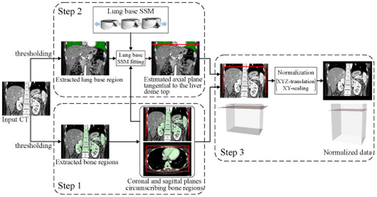
Processes of automated abdominal spatial normalization.
Appendix B. Details of three submodules in single organ segmentation
For simplicity, the organ index k is omitted in the following descriptions.
1. PA-based MAP segmentation
Given target image data I(x), L̂(x) maximizing the posterior probability Prob(L | I) is calculated using PA P(x) and IM H(I) = {HO(I), HB(I)}. The problem is formulated as binary MAP estimation for the target organ and background regions. Using Bayes' theorem, the posterior probability Prob(L | I) is proportional to the product of likelihood Prob(I | L) and the prior probability Prob(L). Using P(x), Prob(L) is defined as
| (B.1) |
We assume that each I(x) is conditionally independent. The likelihood Prob(I(x) | L(x)) is defined as
| (B.2) |
L̂(x)is calculated by
| (B.3) |
After opening and closing using spherical structuring element of radius ρ are applied to L̂(x), we obtain the PA-based segmentation result, which is denoted as LPA(x). Optimization of radius ρ is described in Section 3.3.
2. SSM-based refinement
SSM-based refinement of LPA(x) is performed by repeating edge point detection on the binarized likelihood image and fitting SSM to the detected edge points (Okada et al., 2008). As a threshold value of the likelihood image, the value was calculated to satisfy the following: the intensity distribution within the region of binarized likelihood image include the intensity distribution of target organ and not include that of the background region as possible. To do so, the threshold value of likelihood image is determined by following way. Figure B.2 shows the method for determining the threshold value for the likelihood image. Let p be the probability value of HO(I). The true positive fraction TPF(p) and false positive fraction FPF(p) of HO(I) at the probability p are defined as TPF(p) = Σi HO(I = i) [HO(I = i) ≥ p] and FPF(p) = Σi HB(I = i)[HO(I = i) ≥ p], respectively, where [·] denotes an Iverson bracket, which is equal to 1 when the logical condition enclosed is true and 0 otherwise (Fig. B.2). The threshold value for the likelihood image p̂ is defined as
| (B.4) |
where Youden's index (TPF(p) − FPF(p)) (Youden, 1950) is maximized.
Figure B.2.
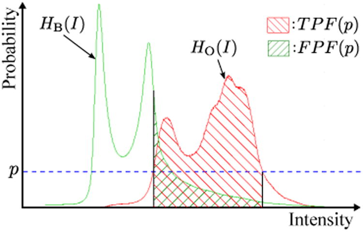
Determination of threshold value p̂ for likelihood image. Red and green plots are the histograms of object HO(I) and background HB(I), respectively. Given a probability value p, TPF(p), FPF(p), and Youden's index can be calculated. The threshold value for likelihood image p̂ is determined so that Youden's index is maximized.
Let M(b) be the surface model generated by SSM s(b) and Xlikelihood the contour points of the binarized likelihood image by the threshold value p̂. We define edge points Xj detected at the j-th iteration as
| (B.5) |
where D(x; M) is the Euclidean distance between point x and the nearest point of x on the surface M, bj−1 is the shape parameter vector of SSM at the (j − 1)-th iteration, and dmax is the maximum distance to limit the search area for edges. In this paper, we used dmax = 20 mm. The maximum distance to limit the search area was also used by Lamecker et al. (2004) to reduce the influence of outliers. The contour points of LPA(x) are used for X1.
Given edge points Xj, the shape parameter vector bj of SSM is defined as
| (B.6) |
where λ is a weight parameter, and CD(b; M(b), Xj) and CM(b) are defined as
| (B.7) |
and
| (B.8) |
respectively, in which |M| denotes the number of vertices of surface M, ‖v‖ the Euclidean norm of vector v, and m the number of principal modes of SSM. The Levenberg-Marquardt algorithm is used for minimization in Eq. (B.6). Optimization of weight parameter λ is described in Section 3.3. The segmentation result of SSM refinement LSSM(x) is obtained by voxelization of the shape model, which is obtained by a fixed number of iterations of edge point detection and fitting to the detected points.
3. Graph-cut refinement
Graph-cut refinement (Boykov and Jolly, 2001) is performed for LSSM. The boundary term and hard constraint in the original formulation (Boykov and Jolly, 2001) are used while the regional term is not used. Let R = {x | LSSM(x) = 1} be the extracted region in LSSM(x). The boundary term B{x,y} is defined as
| (B.9) |
where
is the variance of the intensity value between adjacent voxels, np the total number of pairs of adjacent voxels within R, and N(x) a neighborhood of x. Hard constraint regions for object and background are automatically determined based on segmented region R (while they are manually specified by a user in the original method developed by Boykov and Jolly (2001)). Let H(I; R) be the probability distribution of the intensity histogram within R. The hard constraint regions for object and background
 and ℬ are respectively defined as
| (B.10) |
| (B.11) |
where Rc is the complement of R, pO and pB the values to determine the hard constraint regions for object and background, respectively, and t(p; H(I; R)) = maxt{t | Σi
H(I = i; R)[H(I = i; R) ≥ t] ≥ Z(p)}, in which Z(p) is the probability of a random variable with standard normal distribution
 (0, 1) falling in the range [−p, p]. Optimization of pO and pB is described in Section 3.3.
Appendix C. Training of prediction model using PLSR
Let Xc and Yc be the mean centered matrices of X and Y, respectively. Using PLSR, Yc can be written as
| (C.1) |
where Bpls is the regression coefficient matrix. This matrix can be calculated using the NIPALS algorithm (Yang et al., 2008; Geladi and Kowalski, 1986). The target vector ŷ predicted from the predictor vector x is defined as
| (C.2) |
where μX and μY are the mean vectors of X and Y, respectively. Let X̃i and Ỹi be the datasets except for case i, be the regression coefficient matrix constructed from X̃i and Ỹi, and Bpls,m be the matrix using the first m columns of Bpls. The prediction error εm is defined as
| (C.3) |
where
| (C.4) |
The optimal number of factors of Bpls is defined as
| (C.5) |
Given the predictor vector x, the predicted target vector ŷ is defined as
| (C.6) |
Appendix D. Automated surface subdivision based on canonical correlation analysis
Organ surfaces are recursively subdivided based on a significance level of point-pair correlation within the surface. We use canonical correlation analysis (CCA) to calculate the significance of correlations between two points (Fillard et al, 2007).
Let V0 = {vi} be the vertices of the surface S to be divided and p(u, v) be the significance of correlations between the two points u and v based on CCA. Given the maximum level of division kmax, the processes of the automated surface subdivision are as follows:
p(vi, vj) is calculated among all possible pairs of points (vi, vj)(i ≠ j)in V0.
The level of division k ← 0
- The most uncorrelated point-pair (vV1, vV2) is selected as
(D.1) - All vertices in V0 are separated into the two sets of vertices V1 and V2 based on the significance of the correlations with vV1 and vV2 as follows:
(D.2) (D.3) The sub-shapes S1 and S2 containing only the vertices inV1 and V2 are extracted from S, respectively.
k ← k + 1
The processes 3. to 6. are recursively applied to Si(i = 1, 2) until the level of division reaches kmax.
Once the surface subdivision is performed for the average shape, the surface model represented by SSM can be automatically subdivided using known correspondences.
Footnotes
Publisher's Disclaimer: This is a PDF file of an unedited manuscript that has been accepted for publication. As a service to our customers we are providing this early version of the manuscript. The manuscript will undergo copyediting, typesetting, and review of the resulting proof before it is published in its final citable form. Please note that during the production process errors may be discovered which could affect the content, and all legal disclaimers that apply to the journal pertain.
Contributor Information
Toshiyuki Okada, Email: okada.t@md.tsukuba.ac.jp.
Yoshinobu Sato, Email: yoshi@is.naist.jp.
References
- Aljabar P, Heckemann RA, Hammers A, Hajnal JV, Rueckert D. Multi-atlas based segmentation of brain images: atlas selection and its effect on accuracy. NeuroImage. 2009;46:726–38. doi: 10.1016/j.neuroimage.2009.02.018. [DOI] [PubMed] [Google Scholar]
- Bagci U, Chen X, Udupa JK. Hierarchical Scale-Based Multiobject Recognition of 3-D Anatomical Structures. IEEE Trans Med Imaging. 2012;31:777–89. doi: 10.1109/TMI.2011.2180920. [DOI] [PubMed] [Google Scholar]
- Boykov Y, Jolly MP. Interactive graph cuts for optimal boundary & region segmentation of objects in N-D images. Proc Eighth IEEE Int Conf Comput Vis. 2001:105–12. [Google Scholar]
- Camara O, Colliot O, Bloch I. Computational modeling of thoracic and abdominal anatomy using spatial relationships for image segmentation. Real-Time Imaging. 2004;10:263–73. [Google Scholar]
- Cerrolaza JJ, Herrezuelo NC, Villanueva A, Cabeza R, González Ballester MA, Linguraru MG. Multiresolution Hierarchical Shape Models in 3D Subcortical Brain Structures. In: Mori K, Sakuma I, Sato Y, Barillot C, Navab N, editors. Med Image Comput Comput Assist Interv. Vol. 8150. Springer; Berlin Heidelberg: 2013. pp. 641–8. [DOI] [PubMed] [Google Scholar]
- Cerrolaza JJ, Villanueva A, Cabeza R. Hierarchical statistical shape models of multiobject anatomical structures: application to brain MRI. IEEE Trans Med Imaging. 2012;31:713–24. doi: 10.1109/TMI.2011.2175940. [DOI] [PubMed] [Google Scholar]
- Chen X, Summers RM, Cho M, Bagci U, Yao J. An Automatic Method for Renal Cortex Segmentation on CT Images. Acad Radiol. 2012;19:562–70. doi: 10.1016/j.acra.2012.01.005. [DOI] [PMC free article] [PubMed] [Google Scholar]
- Chu C, Oda M, Kitasaka T, Misawa K, Fujiwara M, Hayashi Y, Nimura Y, Rueckert D, Mori K. Multi-organ Segmentation Based on Spatially-Divided Probabilistic Atlas from 3D Abdominal CT Images. In: Mori K, Sakuma I, Sato Y, Barillot C, Navab N, editors. Med Image Comput Comput Assist Interv. Vol. 8150. Springer; Berlin Heidelberg: 2013. pp. 165–72. [DOI] [PubMed] [Google Scholar]
- Criminisi A, Robertson D, Konukoglu E, Shotton J, Pathak S, White S, Siddiqui K. Regression forests for efficient anatomy detection and localization in computed tomography scans. Med Image Anal. 2013;17:1293–1303. doi: 10.1016/j.media.2013.01.001. [DOI] [PubMed] [Google Scholar]
- Cuingnet R, Prevost R, Lesage D, Cohen LD, Mory B, Ardon R. Automatic Detection and Segmentation of Kidneys in 3D CT Images Using Random Forests. In: Ayache N, Delingette H, Golland P, Mori K, editors. Med Image Comput Comput Assist Interv. Vol. 7512. Springer; Berlin Heidelberg: 2012. pp. 66–74. [DOI] [PubMed] [Google Scholar]
- Dice LR. Measures of the Amount of Ecologic Association Between Species. Ecology. 1945;26:297–302. [Google Scholar]
- Duquette AA, Jodoin PM, Bouchot O, Lalande A. 3D segmentation of abdominal aorta from CT-scan and MR images. Comput Med Imaging Graph. 2012;36:294–303. doi: 10.1016/j.compmedimag.2011.12.001. [DOI] [PubMed] [Google Scholar]
- Fillard P, Pennec X, Thompson P, Ayache N. Evaluating Brain Anatomical Correlations via Canonical Correlation Analysis of Sulcal Lines. Proceedings of MICCAI 2007 workshop on statistical registration: Pair-wise and Group-wise Alignment and Atlas Formation 2007 [Google Scholar]
- Freiman M, Kronman A, Esses S, Joskowicz L, Sosna J. Non-parametric Iterative Model Constraint Graph min-cut for Automatic Kidney Segmentation. In: Jiang T, Navab N, Pluim J, Viergever M, editors. Med Image Comput Comput Assist Interv. Vol. 6363. Springer; Berlin Heidelberg: 2010. pp. 73–80. [DOI] [PubMed] [Google Scholar]
- Fukuda N, Nakamoto M, Okada T, Shoji S, Ukimura O, Gill IS, Hori M, Sato Y. Automated CT segmentation of cancerous kidneys by combining tumor detectors. JAMIT Annual Meeting 2013. 2013 in Japanese. [Google Scholar]
- Geladi P, Kowalski BR. Partial least-squares regression: a tutorial. Anal Chim Acta. 1986;185:1–17. [Google Scholar]
- Glocker B, Pauly O, Konukoglu E, Criminisi A. Joint Classification-Regression Forests for Spatially Structured Multi-object Segmentation. In: Fitzgibbon A, Lazebnik S, Perona P, Sato Y, Schmid C, editors. Comput Vis - ECCV 2012. Vol. 7575. Springer; Berlin Heidelberg: 2012. pp. 870–81. [Google Scholar]
- Hammon M, Cavallaro A, Erdt M, Dankerl P, Kirschner M, Drechsler K, Wesarg S, Uder M, Janka R. Model-Based Pancreas Segmentation in Portal Venous Phase Contrast-Enhanced CT Images. J Digit Imaging. 2013;26:1082–90. doi: 10.1007/s10278-013-9586-7. [DOI] [PMC free article] [PubMed] [Google Scholar]
- Hanaoka S, Masutani Y, Nemoto M, Nomura Y, Yoshikawa T, Hayashi N, Yoshioka N, Ohtomo K. Probabilistic Modeling of Landmark Distances and Structure for Anomaly-proof Landmark Detection. In: Pennec X, Joshi S, Nielsen M, editors. Proceedings of the Third International Workshop on Mathematical Foundations of Computational Anatomy - Geometrical and Statistical Methods for Modelling Biological Shape Variability. 2011. pp. 159–69. [Google Scholar]
- Heimann T, van Ginneken B, Styner MA, Arzhaeva Y, Aurich V, Bauer C, Beck A, Becker C, Beichel R, Bekes G, Bello F, Binnig G, Bischof H, Bornik A, Cashman PMM, Chi Y, Cordova A, Dawant BM, Fidrich M, Furst JD, Furukawa D, Grenacher L, Hornegger J, Kainmüller D, Kitney RI, Kobatake H, Lamecker H, Lange T, Lee J, Lennon B, Li R, Li S, Meinzer HP, Nemeth G, Raicu DS, Rau AM, van Rikxoort EM, Rousson M, Rusko L, Saddi KA, Schmidt G, Seghers D, Shimizu A, Slagmolen P, Sorantin E, Soza G, Susomboon R, Waite JM, Wimmer A, Wolf I. Comparison and evaluation of methods for liver segmentation from CT datasets. IEEE Trans Med Imaging. 2009;28:1251–65. doi: 10.1109/TMI.2009.2013851. [DOI] [PubMed] [Google Scholar]
- Heimann T, Meinzer HP. Statistical shape models for 3D medical image segmentation: a review. Med Image Anal. 2009;13:543–63. doi: 10.1016/j.media.2009.05.004. [DOI] [PubMed] [Google Scholar]
- Hirayama S, Okada T, Hori M, Tomiyama N, Sato Y. Automated segmentation of the upper digestive tract from abdominal contrast-enhanced CT data using hierarchical statistical modeling of organ inter-relations. Inst Electron Inf Commun Eng, Tech Rep. 2013;112:149–154. in Japanese. [Google Scholar]
- Iglesias JE, Sabuncu MR, Leemput KV. A unified framework for cross-modality multi-atlas segmentation of brain MRI. Med Image Anal. 2013;17:1181–91. doi: 10.1016/j.media.2013.08.001. [DOI] [PMC free article] [PubMed] [Google Scholar]
- Isgum I, Staring M, Rutten A, Prokop M, Viergever MA, van Ginneken B. Multi-atlas-based segmentation with local decision fusion– application to cardiac and aortic segmentation in CT scans. IEEE Trans Med Imaging. 2009;28:1000–10. doi: 10.1109/TMI.2008.2011480. [DOI] [PubMed] [Google Scholar]
- Jaccard P. Étude comparative de la distribution florale dans une portion des Alpes et des Jura. Bull Soc Vaud Sci Nat. 1901;37:547–79. [Google Scholar]
- Kainmüller D, Lange T, Lamecker H. Shape constrained automatic segmentation of the liver based on a heuristic intensity model. Proc MICCAI Workshop on 3-D Segmentation in the Clinic: A Grand Challenge. 2007:109–16. [Google Scholar]
- Khalifa F, Gimel'farb G, El-Ghar M, Sokhadze G, Manning S, McClure P, Ouseph R, El-Baz A. A new deformable model-based segmentation approach for accurate extraction of the kidney from abdominal CT images. 18th IEEE Int Conf Image Process (ICIP) 2011:3393–6. [Google Scholar]
- Kohlberger T, Uzunbaş MG, Alvino C, Kadir T, Slosman DO, Funka-Lea G. Organ Segmentation with Level Sets Using Local Shape and Appearance Priors. In: Yang GZ, Hawkes D, Rueckert D, Noble A, Taylor C, editors. Med Image Comput Comput Assist Interv. Vol. 5762. Springer; Berlin Heidelberg: 2009. pp. 34–42. [DOI] [PubMed] [Google Scholar]
- Kurkure U, Avila-Montes O, Kakadiaris I. Automated segmentation of thoracic aorta in non-contrast CT images. 5th IEEE Int Symp Biomed Imaging: From Nano to Macro. 2008:29–32. [Google Scholar]
- Lamecker H, Lange T, Seebaß M. Technical report. Zuse Institue; Berlin: 2004. Segmentation of the liver using a 3D statistical shape model. [Google Scholar]
- Ling H, Zhou S, Zheng Y, Georgescu B, Suehling M, Comaniciu D. Hierarchical, learning-based automatic liver segmentation. IEEE Conf Comput Vis Pattern Recognit. 2008:1–8. [Google Scholar]
- Linguraru M, Richbourg W, Liu J, Watt J, Pamulapati V, Wang S, Summers RM. Tumor Burden Analysis from CT Data of Diseased Patients via Automated Liver and Tumor Segmentation. IEEE Trans Med Imaging. 2012a;31:1965–76. doi: 10.1109/TMI.2012.2211887. [DOI] [PMC free article] [PubMed] [Google Scholar]
- Linguraru M, Sandberg J, Li Z, Shah F, Summers R. Automated Segmentation and Quanitification of Liver and Spleen from CT Images using Normalized Probabilistic Atlases and Enhancement Estimation. Med Phys. 2010;37:771–83. doi: 10.1118/1.3284530. [DOI] [PMC free article] [PubMed] [Google Scholar]
- Linguraru MG, Pura Ja, Pamulapati V, Summers RM. Statistical 4D graphs for multi-organ abdominal segmentation from multiphase CT. Med Image Anal. 2012b;16:904–14. doi: 10.1016/j.media.2012.02.001. [DOI] [PMC free article] [PubMed] [Google Scholar]
- Massoptier L, Casciaro S. Fully Automatic Liver Segmentation through Graph-Cut Technique. 29th Annu Int Conf IEEE Eng Med Biol Soc. 2007:5243–6. doi: 10.1109/IEMBS.2007.4353524. [DOI] [PubMed] [Google Scholar]
- Montillo A, Shotton J, Winn J, Iglesias JE, Metaxas D, Criminisi A. Entangled Decision Forests and Their Application for Semantic Segmentation of CT Images. In: Székely G, Hahn H, editors. Inf Process Med Imaging. Vol. 6801. Springer; Berlin Heidelberg: 2011. pp. 184–96. [DOI] [PubMed] [Google Scholar]
- Okada T, Linguraru MG, Hori M, Summers RM, Tomiyama N, Sato Y. Abdominal Multi-organ CT Segmentation Using Organ Correlation Graph and Prediction-Based Shape and Location Priors. In: Mori K, Sakuma I, Sato Y, Barillot C, Navab N, editors. Med Image Comput Comput Assist Interv. Vol. 8151. Springer; Berlin Heidelberg: 2013. pp. 275–82. [DOI] [PubMed] [Google Scholar]
- Okada T, Linguraru MG, Hori M, Suzuki Y, Summers RM, Tomiyama N, Sato Y. Multi-organ segmentation in abdominal CT images. IEEE Annu Int Conf Eng Med Biol Soc, IEEE. 2012a:3986–9. doi: 10.1109/EMBC.2012.6346840. [DOI] [PMC free article] [PubMed] [Google Scholar]
- Okada T, Linguraru MG, Yoshida Y, Hori M, Summers R, Chen YW, Tomiyama N, Sato Y. Abdominal Multi-Organ Segmentation of CT Images Based on Hierarchical Spatial Modeling of Organ Interrelations. In: Yoshida H, Sakas G, Linguraru MG, editors. Abdom Imaging Comput Clin Appl. Vol. 7029. Springer; Berlin Heidelberg: 2012b. pp. 173–80. [Google Scholar]
- Okada T, Shimada R, Hori M, Nakamoto M, Chen YW, Nakamura H, Sato Y. Automated segmentation of the liver from 3D CT images using probabilistic atlas and multilevel statistical shape model. Acad Radiol. 2008;15:1390–403. doi: 10.1016/j.acra.2008.07.008. [DOI] [PubMed] [Google Scholar]
- Park H, Bland PH, Meyer CR. Construction of an abdominal probabilistic atlas and its application in segmentation. IEEE Trans Med Imaging. 2003;22:483–92. doi: 10.1109/TMI.2003.809139. [DOI] [PubMed] [Google Scholar]
- Sanchez-Castro F, Thierry L, Mory B. Automatic Inferior Vena Cava Segmentation for Hepatic Surgery Planning in Contrast-Enhanced CT Images. Int J Comput Assist Radiol Surg. 2010:S118–S119. [Google Scholar]
- Seifert S, Barbu A, Zhou SK, Liu D, Feulner J, Huber M, Suehling M, Cavallaro A, Comaniciu D. Hierarchical parsing and semantic navigation of full body CT data. Proceedings of SPIE. 2009:725902–725902–8. [Google Scholar]
- Shimizu A, Kimoto T, Kobatake H, Nawano S, Shinozaki K. Automated pancreas segmentation from three-dimensional contrast-enhanced computed tomography. Int J Comput Assist Radiol Surg. 2010;5:85–98. doi: 10.1007/s11548-009-0384-0. [DOI] [PubMed] [Google Scholar]
- Shimizu A, Ohno R, Ikegami T, Kobatake H, Nawano S, Smutek D. Segmentation of multiple organs in non-contrast 3D abdominal CT images. Int J Comput Assist Radiol Surg. 2007;2:135–42. [Google Scholar]
- Suzuki M, Linguraru M, Okada K. Multi-Organ Segmentation with Missing Organs in Abdominal CT Images. In: Ayache N, Delingette H, Golland P, Mori K, editors. Med Image Comput Comput Assist Interv. Vol. 7512. Springer; Berlin Heidelberg: 2012a. pp. 418–25. [DOI] [PubMed] [Google Scholar]
- Suzuki M, Linguraru M, Summers R, Okada K. Analyses of missing organs in abdominal multi-organ segmentation. In: Yoshida H, Sakas G, Linguraru M, editors. Abdom Imaging Comput Clin Appl. Vol. 7029. Springer; Berlin Heidelberg: 2012b. pp. 256–263. [Google Scholar]
- Tomoshige S, Oost E, Shimizu A, Watanabe H, Nawano S. A conditional statistical shape model with integrated error estimation of the conditions; Application to liver segmentation in non-contrast CT images. Med Image Anal. 2014;18:130–143. doi: 10.1016/j.media.2013.10.003. [DOI] [PubMed] [Google Scholar]
- Umetsu S, Shimizu A, Watanabe H, Kobatake H, Nawano S. An automated segmentation algorithm for ct volumes of livers with atypical shapes and large pathological lesions. IEICE Trans Inf Syst. 2014;97:951–963. [Google Scholar]
- Uzunbaş MG, Soldea O, Unay D, Cetin M, Unal G, Erçil A, Ekin A. Coupled nonparametric shape and moment-based intershape pose priors for multiple basal ganglia structure segmentation. IEEE Trans Med Imaging. 2010;29:1959–78. doi: 10.1109/TMI.2010.2053554. [DOI] [PubMed] [Google Scholar]
- Wolz R, Chu C, Misawa K, Fujiwara M, Mori K, Rueckert D. Automated abdominal multi-organ segmentation with subject-specific atlas generation. IEEE Trans Med Imaging. 2013;32:1723–30. doi: 10.1109/TMI.2013.2265805. [DOI] [PubMed] [Google Scholar]
- Yang J, Staib L, Duncan J. Neighbor-constrained segmentation with level set based 3-D deformable models. IEEE Trans Med Imaging. 2004;23:940–8. doi: 10.1109/TMI.2004.830802. [DOI] [PMC free article] [PubMed] [Google Scholar]
- Yang YM, Rueckert D, Bull AMJ. Predicting the shapes of bones at a joint: application to the shoulder. Comput Methods Biomech Biomed Eng. 2008;11:19–30. doi: 10.1080/10255840701552721. [DOI] [PubMed] [Google Scholar]
- Yokota F, Okada T, Takao M, Sugano N, Tada Y, Tomiyama N, Sato Y. Automated CT segmentation of diseased hip using hierarchical and conditional statistical shape models. In: Mori K, Sakuma I, Sato Y, Barillot C, Navab N, editors. Med Image Comput Comput Assist Interv. Vol. 8151. Springer; Berlin Heidelberg: 2013. pp. 190–7. [DOI] [PubMed] [Google Scholar]
- Yoshida Y, Okada T, Hori M, Chen YW, Tomiyama N, Sato Y. Hierarchical spatial normalization based on multi-organ interrelation for atlas-based segmentation: application to gallbladder segmentation from abdominal CT data. Int J Comput Assist Radiol Surg. 2011:S326–S327. [Google Scholar]
- Youden WJ. Index for rating diagnostic tests. Cancer. 1950;3:32–35. doi: 10.1002/1097-0142(1950)3:1<32::aid-cncr2820030106>3.0.co;2-3. [DOI] [PubMed] [Google Scholar]
- Zhang X, Tian J, Deng K, Wu Y, Li X. Automatic Liver Segmentation Using a Statistical Shape Model With Optimal Surface Detection. IEEE Trans Biomed Eng. 2010;57:2622–6. doi: 10.1109/TBME.2010.2056369. [DOI] [PubMed] [Google Scholar]
- Zhou J, Huang W, Zhang J, Yang T, Liu J, Chui CK, Chang S. Segmentation of gallbladder from CT images for a surgical training system. 3rd Int Conf Biomed Eng Inform (BMEI) 2010:536–40. [Google Scholar]
- Zhou X, Kitagawa T, Hara T, Fujita H, Zhang X, Yokoyama R, Kondo H, Kanematsu M, Hoshi H. Constructing a Probabilistic Model for Automated Liver Region Segmentation Using Non-contrast X-Ray Torso CT images. In: Larsen R, Nielsen M, Sporring J, editors. Med Image Comput Comput Assist Interv. Vol. 4191. Springer; Berlin Heidelberg: 2006. pp. 856–63. [DOI] [PubMed] [Google Scholar]
Associated Data
This section collects any data citations, data availability statements, or supplementary materials included in this article.


