ppcor: An R Package for a Fast Calculation to Semi-partial Correlation Coefficients

Abstract

Lack of a general matrix formula hampers implementation of the semi-partial correlation, also known as part correlation, to the higher-order coefficient. This is because the higher-order semi-partial correlation calculation using a recursive formula requires an enormous number of recursive calculations to obtain the correlation coefficients. To resolve this difficulty, we derive a general matrix formula of the semi-partial correlation for fast computation. The semi-partial correlations are then implemented on an R package ppcor along with the partial correlation. Owing to the general matrix formulas, users can readily calculate the coefficients of both partial and semi-partial correlations without computational burden. The package ppcor further provides users with the level of the statistical significance with its test statistic.

1. Introduction

The partial and semi-partial (also known as part) correlations are used to express the specific portion of variance explained by eliminating the effect of other variables when assessing the correlation between two variables (James, 2002; Johnson and Wichern, 2002; Whittaker, 1990). The great number of studies have been published using either partial or semi-partial correlations in many areas including cognitive psychology (e.g., Baum and Rude, 2013), genomics (e.g., Kim and Yi, 2007; Fang et al., 2009; Zhu and Zhang, 2009), medicine (e.g., Vanderlinden et al., 2013), and metabolomics (e.g., Kim et al., 2012; Kim and Zhang, 2013).

The partial correlation can be explained as the association between two random variables after eliminating the effect of all other random variables, while the semi-partial correlation eliminates the effect of a fraction of other random variables, for instance, removing the effect of all other random variables from just one of two interesting random variables. The rationale for the partial and semi-partial correlations is to estimate a direct relationship or association between two random variables. The brief explanation follows to describe the main difference among the correlation, the partial correlation and the semi-partial correlation. Suppose there are three random variables (or vectors), X, Y and Z, and we are interested in the relationship (or association) between X and Y, for illustration purposes. Three situations are taken into consideration as shown in Figure 1. The figure describes three cases that (a) Z is correlated with none of X and Y, (b) only the random variable Y is correlated with Z and (c) Z is correlated with both X and Y. Because Z is independent of both X and Y in Figure 1(a), the correlation, partial correlation and semi-partial correlation all should theoretically have the identical value. When only Y is correlated with Z as shown in Figure 1(b), the partial correlation is exactly same as the semi-partial correlation, but is different from the correlation. However, in case of Figure 1(c), all three correlations are different from each other. For more details on the partial and semi-partial correlations, refer to James (2002) and Whittaker (1990).

Figure 1.

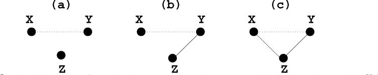
Graphical illustration of partial and semi-partial correlations among the three random variables X, Y, and Z

Several R packages have been developed only for the partial correlation. The R package corpcor (Schafer and Strimmer, 2005) provides the function cor2pcor() for computing partial correlation from correlation matrix and vice versa. The function ggm.estimate.pcor(), which is built in the package GeneNet (Schafer and Strimmer, 2005), allows users to estimate the partial correlation for graphical Gaussian models. The package PCIT (Watson-Haigh et al., 2010) provides an algorithm for calculating the partial correlation coefficient with information theory. The function partial.cor() is included in Rcmdr (Fox, 2005) package for computing partial correlations. The package parcor (Kramer et al., 2009) can be used for regularized estimation of partial correlation matrices. The qp (Castelo and Roverato, 2006) package provides users with q-order partial correlation graph search algorithm. The R package space (Peng et al., 2009) can be used for sparse partial correlation estimation. However, none of these packages provide the level of significance for the partial correlation coefficient such as p-value and statistic. Furthermore, to our knowledge, there exists no R package for semi-partial correlation calculation.

On the other hand, there is no attempt to reduce the computational burden of the higher-order semi-partial correlation coefficients, while the higher-order partial correlation coefficients can be easily calculated using the inverse variance-covariance matrix. This means that a recursive formula (e.g., see Equation (2.2)) should be used for the higher-order semi-partial correlation calculation, hampering the use of the semi-partial correlation for high-dimensional data, such as ‘omics’ data, due to its expensive computation.

For these reasons, we derive a general matrix formula for the semi-partial correlation calculation (see Equation (2.6)). Using this general matrix formula, the semi-partial correlation coefficient can be simple but fast calculated. In order for the partial and the semi-partial correlations to be used practically, an R package ppcor is further developed in the R system for statistical computing (R Development Core Team, 2015). It provides a means for fast computing partial and semi-partial correlation as well as the level of statistical significance. The package ppcor is publicly available from CRAN at http://CRAN.r-project.org/package=ppcor and it is also available in the Supplementary Material at CSAM homepage (http://csam.or.kr).

2. Partial and Semi-partial Correlations

Consider the random vector X = (x₁, x₂, …, x_i, …, x_n)′ where |X| = n. We denote the variance of a variable random x_i and the covariance between two random variables x_i and x_j as v_i (= var(x_i)) and c_ij (= cov(x_i, xj)), respectively. The variance-covariance matrices of random vectors X and X_S (S ⊂ {1, 2, …, n} and |S| < n) are denoted by C_X and C_S, respectively, where X_S is a random sub-vector of the random vector X. The correlation between two random variables x_i and x_j is denoted by $r_{ij}=\frac{c_{ij}}{\sqrt{v_i}\sqrt{v_j}}\left(=\mathit{corr}\left(x_i,x_j\right)\right)$.

Definition 1

The partial correlation of x_i and x_j given x_k is

$$r_{ij|k}=\frac{r_{ij}-r_{ik}{r}_{jk}}{\sqrt{1-r_{ik}^2}\sqrt{1-r_{jk}^2}}$$ (2.1)

and the semi-partial correlation of x_i with x_j given x_k is

$$r_{i\left(j|k\right)}=\frac{r_{ij}-r_{ik}{r}_{jk}}{\sqrt{1-r_{jk}^2}}.$$ (2.2)

Whittaker (1990) defined the partial correlation using the correlation between two residuals. In fact, we can easily see that the definition in Whittaker (1990) is equivalent to the definition in Equation (2.1). Using the above definition, we can readily obtain another version of the definitions of the partial and the semi-partial correlation coefficients as follows.

Corollary 1

The partial correlation of x_i and x_j given x_k, $r_{\mathit{ij}|k}$, is equal to

$$\mathit{corr}\left(\mathit{resid}\left(i|k\right),\mathit{resid}\left(j|k\right)\right)=\frac{c_{ij}-c_{ik}{v}_k^{-1}{c}_{kj}}{\sqrt{v_i-c_{ik}{v}_k^{-1}{c}_{ki}}\sqrt{v_j-c_{jk}{v}_k^{-1}{c}_{kj}}}$$ (2.3)

and the semi-partial correlation of x_i with x_j given x_k, $r_{i\left(j\right|k)}$, is equal to

$$r_{ij|k}\frac{\sqrt{\mathit{var}\left(\mathit{resid}\left(i|k\right)\right)}}{\sqrt{v_i}}=\frac{c_{ij}-c_{ik}{v}_k^{-1}{c}_{kj}}{\sqrt{v_i}\sqrt{v_j-c_{jk}{v}_k^{-1}{c}_{kj}}},$$ (2.4)

where $\mathit{resid}\left(i|k\right)=x_i-{\widehat{x}}_i\left(x_k\right)\text{and}{\widehat{x}}_i\left(x_k\right)=c_{ik}{v}_k^{-1}{x}_k$.

Note that the proof of Corollary 1 is omitted since it is straightforward. Corollary 1 can be further generalized to the case that there are two or more given variables. In other words, it can be extended to the higher-order partial and the higher-order semi-partial correlations. To do this, we need to consider the inverse variance-covariance matrix of X, $D_X=C_X^{-1}$. For the simplicity’s sake, we denote D_X as [d_ij] and C_X as [c_ij], where d_ij and c_ij are the (i, j)-th cell of the matrices D_X and C_X, respectively, and 1 ≤ i, j ≤ n. Then the partial correlation between two variables given a set of variables can be calculated by the following lemma.

Lemma 1. (Whittaker, 1990)

The partial correlation of x_i and x_j given a random vector X_S (= X_(i,j)), r_ij|S, is equal to

$$-\frac{d_{ij}}{\sqrt{d_{ii}}\sqrt{d_{jj}}},$$ (2.5)

where X_S (= X_(i,j)) is the random sub-vector of X after removing the random variables x_i and x_j and its size is |S| (= |X| −2).

Most R packages for calculation of the partial correlation use the matrix-based calculation which is based on Equation (2.5), since this method is much less computationally expensive than the method based on Equation (2.1). In this case, we have to calculate the inverse variance-covariance matrix D_X in order to obtain the partial correlations for all pairs of the random variables of X. Fortunately, it can be easily obtained with a simple code in R. For example, the partial correlation of x_i and x_j given X_(i,j) of X is the (i, j)-th cell of the following matrix:

R> -cov2cor(solve(cov(X)))

However, there is no matrix-based mathematical formula for the semi-partial correlation. Without a general matrix formula, users have to calculate the higher-order semi-partial correlation through a recursive formula in Equation (2.2), which is time-consuming for high-dimensional data. Therefore, it is highly desirable to have a general matrix formula for the fast higher-order semi-partial correlation calculation. In the next theorem, we drive a matrix-based mathematical formula for the semi-partial correlation calculation.

Theorem 1

The semi-partial correlation of x_i with xj given a random vector X_S (= X_(i,j)), r_i(j|S), is equal to

$$r_{ij|S}\frac{1}{\sqrt{d_{ii}-d_{ij}{d}_{jj}^{-1}{d}_{ji}}}\frac{1}{c_{ii}}.$$ (2.6)

Proof

By Equation (2.4), we have the following equation

$$r_{i\left(j|S\right)}=r_{ij|S}\frac{\sqrt{\mathit{var}\left(\mathit{resid}\left(i|S\right)\right)}}{\sqrt{v_i}}$$ (2.7)

Then, using Equation (2.7) and Lemma 1, we have

$$\begin{array}{c}{r}_{i\left(j\right|S)}=-\frac{d_{\mathit{ij}}}{\sqrt{d_{\mathit{ii}}}}\frac{\sqrt{\left|C_X\right|}}{\sqrt{\left|C_S\right|}\sqrt{c_{\mathit{ii}}}}\\ =-\frac{d_{\mathit{ij}}}{\sqrt{d_{\mathit{ii}}}\sqrt{d_{\mathit{jj}}}}\frac{1}{\sqrt{d_{\mathit{ii}}-d_{\mathit{ij}}{d}_{\mathit{jj}}^{-1}{d}_{\mathit{ji}}}}\frac{1}{c_{\mathit{ii}}}\\ =r_{\mathit{ij}|S}\frac{1}{\sqrt{d_{\mathit{ii}}-d_{\mathit{ij}}{d}_{\mathit{jj}}^{-1}{d}_{\mathit{ji}}}}\frac{1}{c_{\mathit{ii}}}.\end{array}$$

Using Theorem 1, we can readily calculate the semi-partial correlation using several lines of an R code. For example, the semi-partial correlation of x_i with x_j given X_(i,j) is the (i, j)-th cell of the matrix obtained in the last line of the following code.

R> cx <- cov(X)
R> dx <- solve(cx)
R> pc <- -cov2cor(dx)
R> diag(pc) <- 1
R> pc/sqrt(diag(cx))/sqrt(abs(diag(dx)-t(t(dxˆ2)/diag(dx))))

It first calculates the variance-covariance matrix of X, which is cx, and its inverse variance-covariance matrix, which is dx. Then the semi-partial correlations are obtained using the partial correlations, which is pc, in the R code above. Note that when the determinant of variance-covariance matrix is numerically zero, the R package ppcor computes its pseudo-inverse using the Moore-Penrose generalized matrix inverse (Penrose, 1995). However, in this case, no statistics and p-values are provided if the number of variables is greater than or equal to the sample size.

While, to our knowledge, no R packages provide the level of statistical significance for partial correlation coefficient, the R package ppcor includes the calculation of statistics and p-values of each correlation coefficient for both partial and semi-partial correlations. Moreover, ppcor provides users with nonparametric partial and semi-partial correlation coefficients based on Kendall’s and Spearman’s rank correlations.

The statistics t_ij|S and t_i(j|S) of the partial and semi-partial correlation of x_i and (with) x_j given x_S (= X_(i,j)) are calculated, based on the works in Weatherburn (1968) and Sheskin (2003), by

$$t_{ij|S}=r_{ij|S}\sqrt{\frac{N-2-g}{1-r_{ij|S}^2}};t_{i\left(j|S\right)}=r_{i\left(j|S\right)}\sqrt{\frac{N-2-g}{1-r_{i\left(j|S\right)}^2}}$$ (2.8)

where N is the sample size and g is the total number of given (or controlled) variables. Using Equation (2.8), their p-values are calculated by

$$p_{ij|S}=2{\mathrm{\Phi }}_t\left(-\left|t_{ij|S}\right|,N-2-g\right);p_{i\left(j|S\right)}=2{\mathrm{\Phi }}_t\left(-\left|t_{i\left(j|S\right)}\right|,N-2-g\right),$$ (2.9)

where Φ_t(·) is the cumulative density function of a Student’s t distribution with the degree of freedom N − 2 − g. It is known that the standard error is $1/\sqrt{N-2-g}$ (Olkin and Finn, 1995; Stanley and Doucouliagos, 2012; Sharma, 2012).

In case of Kendall’s rank correlation, the statistics pare computed by (Abdi, 2007)

$$z_{ij|S}=r_{ij|S}\sqrt{\frac{9(N-\mathrm{g}-2)(N-g+1)}{2(2N-2g+1)}};z_{i\left(j|S\right)}=r_{i\left(j|S\right)}\sqrt{\frac{9(N-2-g)(N-g+1)}{2(2N-2g+1)}}$$ (2.10)

Using Equations (2.10), their p-values are calculated by

$$p_{\mathit{ij}|S}=2\mathrm{\Phi }(-|z_{\mathit{ij}|S}\left|\right);p_{i\left(j\right|S)}=2\mathrm{\Phi }(-|z_{i\left(j\right|S)}\left|\right),$$ (2.11)

where Φ(·) is the cumulative density function of a standard normal distribution. The standard error is $\sqrt{2(2N-2g+1)}/\sqrt{9(N-g-2)(N-g+1)}$ (Abdi, 2007).

3. Examples

The R package ppcor provides users with four functions which are pcor(), pcor.test(), spcor(), and spcor.test(). The function pcor() (spcor()) calculates the partial (semi-partial) correlations of all pairs of two random variables of a matrix or a data frame and provides the matrices of statistics and p-values of each pairwise partial (semi-partial) correlation. In order to compute the pairwise partial (semi-partial) correlation coefficient of a pair of two random variables given one or more random variables, pcor.test() ( spcor.test()) can be also used instead. We can see how to use these functions through the following examples. First the test data, y.data, need to be created after loading the package with the following R codes.

R> library(ppcor)
R> y.data <- data.frame(
+ hl = c(7,15,19,15,21,22,57,15,20,18),
+ disp = c(0,0.964,0,0,0.921,0,0,1.006,0,1.011),
+ deg = c(9,2,3,4,1,3,1,3,6,1),
+ BC = c(1.78e-02,1.05e-06,1.37e-05,7.18e-03,0,0,0,4.48e-03,2.10e-06,0)
+)

This test data, y.data, consists of 10 samples from four variables, hl, disp, deg, and BC. This data set is available from Drummond et al. (2006) and Kim and Yi (2007). The original data cover the relationship between sequence and functional evolutions in yeast proteins. Here we look at only part of the large data for the illustrative purpose. Note that hl, disp, deg, and BC stand for half life, dispensability, degree, and betweenness-centrality, respectively. Please refer to Drummond et al. (2006) and Kim and Yi (2007) for more details.

We can then calculate all pairwise partial correlations of each pair of two variables given other variables with

R> pcor(x=y.data,method=“spearman”)

Then we obtain the following output:

$estimate
	Hl	disp	deg	BC
hl	1.0000000	−0.7647345	−0.1367596	−0.7860646
disp	−0.7647345	1.0000000	−0.4845966	−0.4506273
deg	−0.1367596	−0.4845966	1.0000000	0.4010940
BC	−0.7860646	−0.4506273	0.4010940	1.0000000
$p.value
	Hl	disp	deg	BC
hl	0.00000000	0.02708081	0.7467551	0.02071908
disp	0.02708081	0.00000000	0.2236095	0.26248897
deg	0.74675508	0.22360945	0.0000000	0.32471409
BC	0.02071908	0.26248897	0.3247141	0.00000000
$statistic
	hl	disp	deg	BC
hl	0.0000000	−2.907150	−0.3381686	−3.114899
disp	−2.9071501	0.000000	−1.3569947	−1.236464
deg	−0.3381686	−1.356995	0.0000000	1.072529
BC	−3.1148991	−1.236464	1.0725286	0.000000
$n
[1]	10
$gp
[1]	2
$method
[1]	“spearman”

The output has six values, estimate, which is the partial correlation coefficient, p-value, which is the level of statistical significance, statistic, which is the test statistic for p-value, n, which is the total number of samples, gp, which is the number of given or controlled variables, and method, which is the used correlation method among Pearson’s, Kendall’s, and Spearman’s correlation methods. In case that the users are interested in the partial correlation between hl and disp given deg and BC, we can compute the partial correlation with

R> pcor.test(x=y.data$hl,y=y.data$disp,z=y.data[,c(“deg”,“BC”)]
+, method=“spearman”)

Then we obtain the following output:

$estimate	p.value	statistic	n	gp	Method
1 −0.7647345	0.02708081	−2.90715	10	2	spearman

Similarly, the semi-partial correlations can be calculated with

R> spcor(x=y.data,method=“spearman”)

Then we obtain the following output:

$estimate
	hl	disp	deg	BC
hl	1.00000000	−0.4254609	−0.04949092	−0.4558649
disp	−0.59319449	1.0000000	−0.27689034	−0.2522965
deg	−0.06380762	−0.2560457	1.00000000	0.2023709
BC	−0.42262366	−0.1677612	0.14551866	1.0000000
$p.value
	hl	Disp	deg	BC
hl	0.0000000	0.2933025	0.9073559	0.2562889
disp	0.1211334	0.0000000	0.5067562	0.5466351
deg	0.8806850	0.5404845	0.0000000	0.6307871
BC	0.2968811	0.6912998	0.7309799	0.0000000
$statistic
	hl	disp	deg	BC
hl	0.0000000	−1.1515898	−0.1213762	−1.2545787
disp	−1.8048658	0.0000000	−0.7058372	−0.6386584
deg	−0.1566153	−0.6488095	0.0000000	0.5061789
BC	−1.1422336	−0.4168368	0.3602815	0.0000000
$n
[1]	10
$gp
[1]	2
$method
[1]	“spearman”

The semi-partial correlation of hl with disp given deg and BC is calculated with

R> spcor.test(x=y.data$hl,y=y.data$disp,z=y.data[,c(“deg”,“BC”)]
+, method=“spearman”)

Then we obtain the following output:

estimate	p.value	statistic	n	Gp	Method
1 −0.4254609	0.2933025	−1.15159	10	2	spearman

It should be noted that, if a general matrix formula for the semi-partial correlation is not available, users have to calculate all pairs of each variable with the function spcor.test using two loops. To see how fast the general matrix formula can compute the semi-partial correlation, we compared the computational time by generating a data matrix with the size of 500 × 100 (i.e., the number of variables is 100 and the number of samples 500). When the function spcor() used, the total amount of computation time was 0.02 second, while it took 135.33 second when the function spcor.test() used with two loops. It demonstrates that the general matrix formula dramatically reduce the computational burden of the higher-order semi-partial correlation calculation. Note that this simulation was implemented on a desktop with Intel Core 2 Duo CPU 3.00 GHz.

4. Conclusions

A general matrix formula for the semi-partial correlation is derived. Lack of this general matrix formula has hampered implantation of the higher-order semi-partial correlation for high-dimensional ‘omics’ data analysis because it requires an enormous number of recursive calculations to obtain the correlation coefficient when using a recursive formula in Equation (2.2). However, using the derived matrix formula in Theorem 1, we can clearly see that the higher-order semi-partial correlation coefficient is calculated as simple but fast as the partial correlation does. The developed R package ppcor further provides users not only with a function to readily calculate the higher-order both partial and semi-partial correlations but also with statistics and p-values of the correlation coefficients.

5. Computational Details

The results in this paper were obtained using R 3.2.2 with the package ppcor. R and the ppcor package are available from CRAN at “http://CRAN.R-Project.org/ and in the Supplementary Material at CSAM homepage (http://csam.or.kr). Note that, in this latest version of the package R, the p-values for Pearsons and Spearmans correlations are calculated based on the t-distribution and the Moore-Penrose generalized inverse matrix will be used when variance-covariance matrix is singular.

References

- Abdi H. Kendall rank correlation. In: Salkind NJ, editor. Encyclopedia of Measurement and Statistics. Thousand Oaks (CA): Sage; 2007. pp. 508–510. [Google Scholar]
- Baum ES, Rude SS. Acceptance-enhanced expressive writing prevents symptoms in participants with low initial depression. Cognitive Therapy and Research. 2013;37:35–42. [Google Scholar]
- Castelo R, Roverato A. A Robust Procedure for Gaussian Graphical Model Search from Microarray Data with p Larger than n. J Mach Learn Res. 2006;7:2621–2650. [Google Scholar]
- Drummond DA, Raval A, Wilke CO. A Single Determinant Dominates the Rate of Yeast Protein Evolution. Molecular Biology and Evolution. 2006;23:327–337. doi: 10.1093/molbev/msj038. [DOI] [PubMed] [Google Scholar]
- Fang XZ, Luo L, Reveille JD, Xiong M. Discussion: Why do we test multiple traits in genetic association studies? Journal of the Korean Statistical Society. 2009;38:17–23. doi: 10.1016/j.jkss.2008.10.006. [DOI] [PMC free article] [PubMed] [Google Scholar]
- Fox J. The R Commander: A Basic-statistics Graphical User Interface to R. Journal of Statistical Software. 2005;14:1–42. [Google Scholar]
- James S. Applied Multivariate Statistics for the Social Sciences. Lawrence Erlbaum Associates, Inc; Mahwah, NJ: 2002. [Google Scholar]
- Johnson RA, Wichern DW. Applied Multivariate Statistical Analysis. Prentice Hall; 2002. [Google Scholar]
- Kim S, Yi S. Understanding Relationship between Sequence and Functional Evolution in Yeast Proteins. Genetica. 2007;131:151–156. doi: 10.1007/s10709-006-9125-2. [DOI] [PubMed] [Google Scholar]
- Kim S, Zhang X. Comparative Analysis of Mass Spectral Similarity Measures on Peak Alignment for Comprehensive Two-Dimensional Gas Chromatography Mass Spectrometry. Computational and Mathematical Methods in Medicine. 2013;2013:509761. doi: 10.1155/2013/509761. [DOI] [PMC free article] [PubMed] [Google Scholar]
- Kim S, Koo I, Jeong J, Wu S, Shi X, Zhang X. Compound identification using partial and semipartial correlations for gas chromatography-mass spectrometry data. Analytical Chemistry. 2012;12:6477–6487. doi: 10.1021/ac301350n. [DOI] [PMC free article] [PubMed] [Google Scholar]
- Kramer N, Schafer J, Boulesteix AL. Regularized Estimation of Large Scale Gene Association Networks using Gaussian Graphical Models. BMC Bioinformatics. 2009;10:384. doi: 10.1186/1471-2105-10-384. [DOI] [PMC free article] [PubMed] [Google Scholar]
- Olkin I, Finn JD. Correlations Redux. Vol. 118. Psychological Bulletin; 1995. pp. 155–164. [Google Scholar]
- Peng J, Wang P, Zhou N, Zhu J. Partial Correlation Estimation by Joint Sparse Regression Models. J Am Stat Assoc. 2009;104:735–746. doi: 10.1198/jasa.2009.0126. [DOI] [PMC free article] [PubMed] [Google Scholar]
- Penrose R. A Generalized Inverse for Matrices. Proc Cambridge Phil Soc. 1995;51:406–413. [Google Scholar]
- R Development Core Team. R: A Language and Environment for Statistical Computing. R Foundation for Statistical Computing; Vienna, Austria: 2011. URL “ http://www.R-project.org/. [Google Scholar]
- Schafer J, Strimmer K. A Shrinkage Approach to Large-scale Covariance Matrix Estimation and Implications for Functional Genomics. Statist Appl Genet Mol Biol. 2005;4:32. doi: 10.2202/1544-6115.1175. [DOI] [PubMed] [Google Scholar]
- Schafer J, Strimmer K. An Empirical Bayes Approach to Inferring Large-scale Gene Association Networks. Bioinformatics. 2005;21:754–764. doi: 10.1093/bioinformatics/bti062. [DOI] [PubMed] [Google Scholar]
- Sharma JK. Business Statistics. Pearson Education; India: 2012. [Google Scholar]
- Sheskin DJ. Handbook of Parametric and Nonparametric Statistical Procedures. Third. CRC Press; 2003. [Google Scholar]
- Stanley TD, Doucouliagos H. Meta-Regression Analysis in Economics and Business. Routledge; 2012. [Google Scholar]
- Vanderlinden LA, Saba LM, Kechris K, Miles MF, Hoffman PL, Tabakoff B. Whole brain and brain regional coexpression network interactions associated with predisposition to alcohol consumption. PLoS ONE. 2013;8:e68878. doi: 10.1371/journal.pone.0068878. [DOI] [PMC free article] [PubMed] [Google Scholar]
- Watson-Haigh NS, Kadarmideen HN, Reverter A. PCIT: An R Package for Weighted Gene Co-expression Networks Based on Partial Correlation and Information Theory Approaches. Bioinformatics. 2010;26:411–413. doi: 10.1093/bioinformatics/btp674. [DOI] [PubMed] [Google Scholar]
- Weatherburn CE. A first course mathematical statistics. Cambridge; 1968. [Google Scholar]
- Whittaker J. Graphical Models in Applied Multivariate Statistics. John Wiley & Sons; 1990. [Google Scholar]
- Zhu WS, Zhang HP. Why do we test multiple traits in genetic association studies? Journal of the Korean Statistical Society. 2009;38:1–10. doi: 10.1016/j.jkss.2008.10.006. [DOI] [PMC free article] [PubMed] [Google Scholar]
Associated Data
This section collects any data citations, data availability statements, or supplementary materials included in this article.