Transmission network of the 2014–2015 Ebola epidemic in Sierra Leone

Abstract

Understanding the growth and spatial expansion of (re)emerging infectious disease outbreaks, such as Ebola and avian influenza, is critical for the effective planning of control measures; however, such efforts are often compromised by data insufficiencies and observational errors. Here, we develop a spatial–temporal inference methodology using a modified network model in conjunction with the ensemble adjustment Kalman filter, a Bayesian inference method equipped to handle observational errors. The combined method is capable of revealing the spatial–temporal progression of infectious disease, while requiring only limited, readily compiled data. We use this method to reconstruct the transmission network of the 2014–2015 Ebola epidemic in Sierra Leone and identify source and sink regions. Our inference suggests that, in Sierra Leone, transmission within the network introduced Ebola to neighbouring districts and initiated self-sustaining local epidemics; two of the more populous and connected districts, Kenema and Port Loko, facilitated two independent transmission pathways. Epidemic intensity differed by district, was highly correlated with population size (r = 0.76, p = 0.0015) and a critical window of opportunity for containing local Ebola epidemics at the source (ca one month) existed. This novel methodology can be used to help identify and contain the spatial expansion of future (re)emerging infectious disease outbreaks.

1. Introduction

The 2014–2015 West African Ebola epidemic is the most severe Ebola outbreak on record. It is believed to have emerged in the Guéckédou region of Guinea during December 2013 [1], and spread to adjacent nations, Liberia in March [2] and Sierra Leone (SL) in May [3,4]. On 25 May 2014, SL reported its first confirmed Ebola case from Kailahun [3], a district on the border, south of Guinea and west of Liberia. By 26 April 2015, 12 371 Ebola cases and 3899 deaths had been reported in SL [5].

Quantification of local growth rates and the geographical spread of (re)emerging infectious diseases are crucial for determining the level and speed of intervention needed to contain an epidemic. Previous studies have used models to simulate and project the propagation of infectious diseases, such as influenza, over national and larger scales and to infer key spatial and temporal epidemiological characteristics of these outbreaks [6–10]. Detailed data resolving population structure and movement are typically needed to calibrate these models; however, such data are not readily available in West Africa [11,12]. Furthermore, observations of Ebola incidence and mortality have been error-laden and biased; indeed, the US Centers for Disease Control and Prevention estimated that only 40% of Ebola cases have been reported [13], and the underreporting rate could vary by region over time. To address these challenges, we here develop a modified patch network model of intermediate complexity for Ebola transmission, which we use in conjunction with a Bayesian inference method, implemented via data assimilation, and district-level incidence data for SL. The combined model-inference system enables simulation and inference of the spatial–temporal spread and characteristics of Ebola in SL.

2. Results

2.1. Framework of the spatio-temporal inference system

A number of epidemiological model structures have been used to simulate Ebola transmission [6,7,13–20]. For Ebola, a person, initially susceptible (S) to the disease, becomes infected when exposed (E) to the virus, then becomes infectious (I) following an incubation period, and is finally removed (R) from the diseased pool owing to recovery or death. Accordingly, we model the propagation of Ebola through a population using a susceptible–exposed–infectious–removed (SEIR) compartmental model [21]. This choice is also based on our previous work indicating that more parsimonious model structures, such as the SEIR model, tend to be more easily optimized than more complex modelling frameworks [22,23]. In a network of multiple districts, residents within each district may contract the disease locally or when traveling to other districts. For instance, new infections at district 1 within a three-district network would occur at a rate of

2.1

where the single digit subscripts are district indices; β is the transmission rate; respectively, denote the number of infectious, susceptible and total number of people present in each district at a given time, i.e. including both local residents and visitors; c₁₁, c₂₁ and c₃₁ are, respectively, the proportions of residents of district 1 that stay local and that travel to districts 2 and 3. The summation (equation (2.1)) includes the number of cases infected locally (first summand) and those infected outside their home district (the second and third summands). This formula assumes that the subpopulation within each district is well mixed, and that new infections in a given district are allocated to local residents and visitors in proportion to their corresponding percentages among the total number of susceptibles; for instance, the total new infection rate in district 1 is 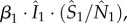with a portion, local residents.

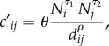
The proportions form a matrix, e.g. 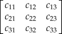for a three-district network, which represents the connectivity among districts. Previous studies [10,24] have computed the raw interdistrict commute flow using a gravity formula

2.2

where N_i and N_j are the population size for the two districts, d_ij is the distance between the two districts, θ is a proportionality constant and the exponents τ₁, τ₂ and ρ together determine the connectivity between the two districts [8,10]. The model is then calibrated using detailed human mobility data (e.g. ground commute flow) and the raw numbers are adjusted to compute the [c_ij] matrix (as detailed in the Material and methods section). As commuter data are not available for SL, we normalize all inputs for population size and distance such that the proportionality constant, θ, which heavily relies on mobility data, is eliminated. Further, we use the area of each district to gauge local mobility (see Material and methods for details of the modified gravity model).

We then couple this modified gravity connection formula with the SEIR network model, and use the ensemble adjustment Kalman filter (EAKF), in conjunction with district-level incidence data, to estimate all state variables (i.e. S, E, I, for each district) and model parameters, including the transmission rate β for each district, the incubation period, the infectious period and the three exponents (τ₁, τ₂ and ρ) for the gravity model. The EAKF [15,23,25–27] is a data assimilation method that uses an ensemble of system replicas to represent the distribution of possible model state and parameter values. It approximates a Bayesian update to the model states and parameters using the observational data and an estimate of the errors in the data. When tested against a model-synthesized dataset resembling the incidence record for SL, our inference method was able to sensibly estimate the state variables and model parameters (see electronic supplementary material, figures S1–S3).

2.2. Model fitting to the district epidemic curves

We applied the inference method to district-level incidence data from the week ending 25 May 2014, the first week of the Ebola epidemic in SL, to the week ending 25 January 2015. Of the 14 SL districts, four in the northwest (Western Area Urban, Western Area Rural, Port Loko and Bombali) recorded the greatest numbers of Ebola cases; the peripheral districts, Bonthe and Pujehun, only had sporadic cases; the remaining districts had moderate outbreaks. The epidemic started from Kailahun [3], then spread west to Kenema and Bo, and then to the rest of SL. Our inference framework is able to recreate the epidemic trajectories for each of the 14 districts (figure 1), and our estimates of key model parameters (table 1) are in line with past studies [28,29]. Note, however, that estimates for the three exponents in the gravity model are not comparable to previous studies [10,30]; this discrepancy is not unexpected as our gravity model is framed differently (see Material and methods).

Figure 1.

Epidemic trajectories and model fits generated by the SEIR-network-EAKF. Weekly incidence records for each district are shown as coloured ‘x’; solid line in the corresponding colour is the average simulated incidence over 300 500-member ensemble runs. Dates shown on the x-axis (dd/mm/yy) are endings of epidemic weeks.

Table 1.

Estimates of key epidemiological parameters. These estimates are aggregated over 300 500-member ensemble runs and shown as mean and standard deviation (parentheses). The SEIR-network-EAKF updated the estimates each week as new weekly incidence data were assimilated; consequently, parameter estimates are shown at four different time points: (i) the onset, defined as the first of three consecutive weeks with non-decreasing numbers of cases; (ii) self-sustained transmission (T_ss), defined as the first week during which over 80% of cases are infected locally; (iii) the maximum epidemic forcing, defined as the week with the highest effective reproductive number R_e; and (iv) the week ending 25 January 2015. R_e was treated as an independent parameter for each district, whereas other parameters were treated as common parameters for all districts. The three time points vary by district; common parameters were estimated at the time points as defined for Western Area Urban. The times for each district are available in the electronic supplementary material, table S2.

	onset	self-sustained (Tss)	maximum epidemic forcing	25 Jan 2015
Re: Bo	1.26 (0.10)	1.31 (0.15)	1.65 (0.17)	1.08 (0.12)
Re: Bombali	1.03 (0.09)	1.10 (0.11)	1.87 (0.12)	0.76 (0.13)
Re: Bonthe	0.79 (0.16)	—	0.85 (0.20)	0.85 (0.20)
Re: Kailahun	1.38 (0.05)	1.56 (0.10)	1.89 (0.18)	0.88 (0.15)
Re: Kambia	0.96 (0.13)	1.11 (0.21)	1.25 (0.21)	1.25 (0.21)
Re: Kenema	1.29 (0.11)	1.92 (0.29)	2.16 (0.19)	0.98 (0.17)
Re: Koinadugu	1.07 (0.11)	1.33 (0.11)	1.33 (0.11)	0.78 (0.12)
Re: Kono	1.00 (0.1)	1.12 (0.13)	1.56 (0.20)	0.96 (0.16)
Re Moyamba	1.06 (0.15)	1.17 (0.17)	1.32 (0.29)	0.44 (0.20)
Re: Port Loko	1.07 (0.09)	1.21 (0.14)	1.82 (0.11)	0.90 (0.23)
Re: Pujehun	1.05 (0.11)	0.93 (0.12)	1.11 (0.15)	0.83 (0.14)
Re: Tonkolili	1.08 (0.10)	1.18 (0.13)	1.56 (0.13)	0.89 (0.12)
Re: Western Area Rural	0.95 (0.10)	0.95 (0.10)	1.85 (0.38)	0.81 (0.11)
Re: Western Area Urban	1.00 (0.10)	1.00 (0.10)	2.22 (0.09)	0.71 (0.25)
incubation period (days)	14.27 (0.94)	14.27 (0.94)	9.64 (1.06)	10.72 (1.11)
infectious period (days)	12.35 (0.79)	12.35 (0.79)	11.32 (0.98)	10.92 (2.53)
gravity model: τ1	0.47 (0.03)	0.47 (0.03)	0.46 (0.04)	0.49 (0.08)
gravity model: τ2	0.50 (0.03)	0.50 (0.03)	0.50 (0.04)	0.51 (0.06)
gravity model: ρ	8.04 (0.37)	8.04 (0.37)	7.93 (0.79)	7.13 (1.28)

2.3. The Ebola transmission network in Sierra Leone

To sort out the transmission path of Ebola from district to district, we compute the number of new cases infected locally versus externally for each district during each week. This computation allows identification of the source of self-sustained local epidemic transmission, as well as the source of the first cases in each district (see electronic supplementary material, table S3). Here, we focus on the former issue. We posit that importation of cases is critical at the very beginning of each local outbreak before transmission is sustained locally. Accordingly, we define the week that a district acquired over 80% of its new infections locally, following the onset of local outbreak, as the onset of self-sustained transmission (T_ss), and identify the district that contributed the largest number of new infections prior to T_ss as the most likely source of infection (see Material and methods and electronic supplementary material for sensitivity analysis).

A clear transmission network emerges (figure 2). Two major transmission paths exist, one spreading from Kailahun to the west and the other from Western Area Urban to the east. The first path emerged on the week ending 25 May 2014 in Kailahun, then spread to adjacent Kenema, over the weeks ending 15 June through 6 July 2014 and produced 21−67% of incidence each week in Kenema during those four weeks prior to T_ss (the range shows the minimum and maximum weekly contributions over the period, same elsewhere). The other adjacent district, Kono, also imported a substantial number of cases (32−41%) during 25 August−7 September 2014, followed by local, sustained transmission. From Kenema, the Ebola epidemic spread farther westwards to Bo (23 June−7 September 2014, 30−72%), southwards to Pujehun (18 August−21 September 2014, 13−27%) and northwards to Tonkolili (4−24 August 2014, 11−14%). These findings are consistent with a recent field investigation that reported the emergence of Ebola epidemic in Sierra Leone, in particular, the spread from Kailahun to Kenema [31].

Figure 2.

Transmission network within Sierra Leone, inferred by the SEIR-network-EAKF. The arrows denote the sources of infection, color-coded by different transmission paths. Transmission paths in red originated in Western Area Urban and those in blue originated in Kailahun. The width of the arrow is proportional to contribution from the source (percentage associated with the end of each arrow) during the dates (dd/mm/yy) indicated next to the percentages. A solid arrow indicates all 300 simulation runs inferred the same path; a dashed arrow indicates only a portion of runs inferred a particular path; the transparency of an arrow also indicates the level of agreement among all runs; greater transparency implies less consensus among runs. Districts labelled in bold are inferred as initial sources of infection by all runs (those attached to solid arrows or no arrows for districts with sporadic cases) or only a fraction of the 300 runs (those attached to dashed arrows). Districts are coloured by their population sizes (indicated in the legend).

The second path initiated from Western Area Urban, which encompasses the Capital Freetown, during 5 July−3 August 2014. This was a relatively quiet period with only two to six cases recorded each week. Ebola incidence then increased rapidly and spread to other districts in western SL. Western Area Rural likely imported a small number of cases from the capital area during the week ending 17 August 2014, prior to T_ss (see electronic supplementary material, figure S5 and figure S7). Ebola emerged in Port Loko, the largest district near Western Area Urban, around the same time; our estimates indicate that 14−17% of Port Loko cases each week during 21 July−3 August 2014 were imported from Western Area Urban. Port Loko then served as a source of transmission for the region: the epidemic spread from there southwards to Moyamba (1−21 September 2014, 14−23%), likely contributed to the spread of Ebola in Kambia (8 September 2014−11 January 2015, 20−62%), and may have seeded Bombali (the week ending 24 August 2014, 17%). The importation to Bombali was less obvious; two-thirds of simulations (n = 300) suggest that the epidemic in the district started locally rather than from Port Loko. These first cases could have originated zoonotically, from outside the country (a source not included in our model), or could have been imported from other districts through longer-distance travel. Regardless, the epidemic then spread from Bombali to Koinadugu (13 October−28 December 2014), and importation from Bombali may have enhanced the transmission in Tonkolili during 1−21 September 2014 (15−17%).

2.4. Spatial expansion characteristics

The two transmission paths converged in Tonkolili; however, it took the Kailahun path three months (25 May−24 August 2014) to reach Tonkolili, compared with less than two months for the Western Area Urban path (28 July−21 September 2014). For both paths, spread occurred more readily to adjacent districts, and a strong source region existed along the path, i.e. Kenema in the east and Port Loko in the west, which borders and facilitated spread to many other districts. This finding indicates that control of outbreaks prior to their spread to these critical, well-connected source districts might delay or reduce importation to surrounding districts and reduce overall case levels. Here, we estimate this window of opportunity as having been approximately one month (25 May−6 July 2014, i.e. the time lag of self-sustained transmission between Kailahun and Kenema) for the Kailahun transmission path, but much shorter for the Western Area Urban path, which traversed a region of greater population and connectedness.

To explore potential differences in local transmission characteristics, we estimated the effective reproductive number, R_e, independently for each district. R_e is the average number of secondary cases arising from a primary case, and thus an indicator of force of infection. To sustain an epidemic, R_e should be above 1. R_e is marginally above 1 for most districts at the onset of local epidemic (table 1); at its maximum, R_e ranges from 0.85 ± 0.20 (mean ± s.d., same elsewhere) in Bonthe, where only sporadic cases were recorded, to 2.22 ± 0.09 in Western Area Urban, where the largest number of cases were reported. These maximum R_e estimates are highly correlated with the population size of each district (r = 0.76, p = 0.0015), and less so with population density (r = 0.46, p = 0.10). Note this finding is not an artefact of the built-in population information in the gravity network connectivity model (see equation (4.2) in Material and methods), as R_e was evaluated at its maximum when local transmission has become the major force of infection. Indeed, the most populated districts (figure 2), i.e. Western Area Urban (16.4% of the nation's total population), Kenema (10.3%), Port Loko (8.8%) and Bombali (7.8%) also had the largest R_e and the highest incidence. This finding indicates that areas with larger populations were more likely to sustain more intense outbreaks and serve as major source regions (e.g. Western Area Urban, Kenema and Port Loko) to neighbouring areas, which is consistent with the transmission network shown in figure 2; it again highlights the importance of early control in these areas. Western Area Rural, where the third largest number of cases was reported, has the second smallest population size. Our estimates indicate that 7.2 ± 2.7% of cases were infected while travelling in the neighbouring epidemic centre, Western Area Urban (table 2).

Table 2.

Transmission contributed from other districts in the network. The numbers of cases infected locally as well as externally from each of the other districts were summed from 25 May 2014 to 25 January 2015; the percentage of imported infections, the most likely source of these infections and the contribution of that source were then calculated. Estimates are aggregated over 300 simulation runs and shown as mean and standard deviation (parentheses).

district	percentage imported (%)	most likely source	percentage from the most likely source (%)
Bo	17 (4.3)	Kenema	14 (2.2)
Bombali	7.2 (3.5)	Port Loko	3.4 (1.8)
Bonthe	20 (12)	Moyamba	12 (5.2)
Kailahun	3.9 (1.2)	Kenema	3.4 (1)
Kambia	37 (14)	Port Loko	33 (11)
Kenema	16 (2.8)	Kailahun	9 (0.95)
Koinadugu	39 (7.9)	Bombali	25 (3.6)
Kono	7.3 (2.1)	Kailahun	3.7 (0.54)
Moyamba	33 (10)	Port Loko	12 (3.6)
Port Loko	18 (5.6)	Western Area Urban	9.4 (2.7)
Pujehun	17 (7.7)	Bo	8.8 (3.8)
Tonkolili	13 (6.3)	Bombali	5.5 (2.4)
Western Area Rural	7.2 (2.7)	Western Area Urban	7.2 (2.7)
Western Area Urban	0.018 (0.023)	Western Area Rural	0.018 (0.023)

For each district, the relative contributions of new infections from other districts varied over the course of the epidemic. For instance, Kenema initially seeded infection in Pujehun; however, later in the epidemic, Bo became the primary source of imported infections for Pujehun. In contrast, some districts remained strong sources throughout the epidemic. For example, Kailahun produced 9.0 ± 0.95% of all cases in Kenema, more than half of all imported cases (table 2). Throughout the epidemic, imported infections remained a significant force of infection for most districts, particularly those with moderate outbreaks, e.g. Koinadugu (39 ± 7.9%), Kambia (37 ± 14%) and Moyamba (33 ± 10%) (table 2).

3. Discussion

During the 2014–2015 Ebola epidemic, a number of issues complicated and potentially obfuscated modelling efforts. First, owing to the scope of the outbreak and the limited surveillance and public health infrastructure in the three most affected West African countries—Guinean, Liberia and SL—observational error, particularly underreporting [13], was unavoidable. This observational error undermines model inference; however, data assimilation methods, such as the EAKF used here, are equipped to handle and explicitly account for observational error [25]. To further allow for observational error effects, we considered six filter settings, running simulations with three different levels of observation error variance (see Material and methods), and used the agreement of inference among the six settings as an indicator of the confidence, or reliability, of the inference (figure 2).

A second concern involves system stochasticity [32], seemingly random processes that arise owing to variations of behaviour or changes in the intensity of intervention measures. To account for these effects, modelling studies have used stochastic model structures [14,17,20,32]. The SEIR network model used here is deterministic; however, the EAKF, used in conjunction with the model, to some extent introduces stochasticity to the system through its ensemble formulation and the random selection of initial state variable and parameter conditions. Indeed, we alternatively built and tested our network model-inference framework using a stochastic SEIR model as the core (see electronic supplementary material). Findings with this alternative stochastic structure generated similar transmission networks and parameter estimates (electronic supplementary material, figure S4 and table S1).

Additional complicating issues, which were not resolved observationally nor represented in the model structure, include differences in transmission risk in different settings (e.g. community, hospital, versus funeral), heterogeneity in population mixing and contact patterns and resulting variations in infection risk at differing geographical scales, potential asymptomatic infections and pre-existing immunity owing to undetected prior circulation of Ebola in the region. Our parsimonious SEIR-network model does not represent these processes; however, despite its simplicity, the system was able to identify major transmission pathways of Ebola spread between districts as well as key characteristics of source regions. For instance, our inference suggests that districts with higher spatial connectivity and larger populations (e.g. Kenema and Port Loko) could be key regional source districts for control. Future work may construct more complex models to investigate the aforementioned issues, were detailed data available to constrain the system. Future work may also apply the model-filter framework to district-level data for Guinea and Liberia, two other countries with intense Ebola transmission, to further test the findings reported here. In addition, our findings may be tested as more detailed viral sequence data, and field investigations become available.

Detailed, timely understanding of the spatial–temporal progression of (re)emerging infectious disease is needed to devise effective control and containment strategies of these outbreaks. Here, we have presented a novel spatial inference system that enables estimation of this spatial–temporal progression of disease. The method uses only district-level incidence data, as well as the area and population of each district and interdistrict distances. All these data can be compiled in near real-time, even during a public health crisis. The core network model presented here uses a normalized, non-dimensional framework that could be easily applied to other diseases and different regions. In the future, this methodology can be used to help public health officials more effectively combat (re)emerging infectious disease.

4. Material and methods

4.1. Data

Weekly incidence data for each of the 14 districts in SL were obtained from the Sierra Leone Ministry of Health and Sanitation. These data were compiled based on each patient's district of origin, as opposed to the district of report. For instance, although the index case in SL was sent for testing at Kenema Government Hospital and reported in Kenema district [1], this patient case was originally from Kailahun district and thus counted as a case for Kailahun. Incidence records are the same as released in the Ebola situation reports [33] and include numbers of suspected, confirmed and probable cases, as defined by the World Health Organization [34], from the week ending 25 May 2014 to the week ending 25 January 2015. We combined these three categories for the simulations reported in the main text.

4.2. Network transmission model

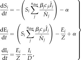
We used an SEIR model to simulate the propagation of Ebola in each district, as our previous work suggests that parsimonious model forms, when used in conjunction with data assimilation methods and observations, can be more easily constrained [22]. Transmission between districts is formulated as a patch network model [35]. We assume that interdistrict transmission occurs when susceptible individuals travel from their home district to other districts and interact with infectious individuals therein. Specifically, the SEIR-network model is formulated as follows

4.1

where the single digit subscripts (i or j) denote district; S_i, E_i, I_i are, respectively, the number of susceptible, exposed and infectious people in district i; β_i is the local transmission rate in district i; α is transmission from outside the network domain, e.g. from outside SL or zoonotic spillover, and is arbitrarily set to one per 10 days in this study (we also tested lower values for α and the difference in model estimates was nominal); Z is the incubation period, D is the infectious period, and both variables are assumed the same for all districts; the basic reproductive number for district i, R_0i, is linked to the transmission rate and infectious period through the relationship R_0i = β_i·D; c_ji is the proportion of residents of district i travelling to district j; a hat sign (^) over a variable denotes the number of people present in the district at a given time point, regardless of home district; is the number of people present in district i at time t, i.e. 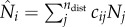with N_j as the population size for district j and n_dist as the total number of districts (i.e. n_dist = 14 for SL); is the number of infectious people present in district i at time t, and is approximated as I_i, because symptomatic individuals are less likely to travel to other districts (except for medical transfer for treatment) and cause infections elsewhere. Note that the approximation of with I_i here is not a choice of convenience; rather, without this approximation, e.g. calculated as done for , symptomatic, infectious individuals are assumed to have the same interdistrict mobility, which is less likely given the severity of Ebola virus disease.

4.3. Modified gravity model

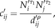
The quantities c_ij (i = 1,…, n_dist, j = 1, … , n_dist) in equation (4.1) form a matrix, C = [c_ij]_{i = 1, …} , n_{dist, j = 1, …} , n_dist, that represents the strength of connection between each district pair. Past studies [8,10,24] have used gravity type formulations to compute interlocale commuter flow rates (e.g. equation (2.2)). Population size for each district in SL and interdistrict distances are publicly available [33,36]; however, mobility data, previously used to calibrate the four parameters in the gravity model (equation (2.2)) [10] are not available for SL. As such, we reframed equation (2.2) using scaled, proportions of population size and distance. In so doing, the proportionality parameter θ, which is heavily dependent on commuter data, is eliminated and equation (2.2) becomes

4.2

where the new dimensionless model inputs are 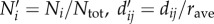(note that d_ii, the within-district distance, is computed as 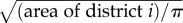, with N_tot as the national population in SL, and a proxy radius for the country). These quantities are then further adjusted, so that the proportions of all residents in a given home-district, i.e. those staying local (c_ii) plus those travelling to each of the other districts (c_ij, i≠j), sum to 1. That is,

4.3

We use the proxy radius for each district (i.e. ) to gauge within-district versus interdistrict mobility, which partly accounts for the effect of population density; that is, residents of more densely populated districts (e.g. the capital region) are less likely to travel to less populated regions (e.g. a remote district). Furthermore, as all inputs are normalized by the characteristic quantities of the country (e.g. area and population of the country), the model framework can be readily applied to other regions. For instance, by using characteristic quantities for Guinea or Liberia, the same model could also be used without relying on mobility data for these countries.

Equations (4.2) and (4.3) are then used to calculate the connectivity matrix needed for equation (4.1). Note, however, by combing equations (2.2), (4.2) and (4.3), the scaling done in equation (4.2) is not necessary, as the normalization in equation (4.3) would cancel out the common factor . The exponents τ₁, τ₂ and ρ, which determine the influence of donor and recipient population size and distance, are estimated by the data assimilation method described below.

4.4. Data assimilation method

We applied the EAKF [15,25] in conjunction with the SEIR-network model and weekly incidence records for all 14 districts. The EAKF uses multiple system replicas, termed ensemble members, to represent the prior and posterior distributions of each state variable and parameter. Each ensemble member is initialized as a random draw from an initial distribution for each of the model state variables and model parameters; it is then propagated per the SEIR-network model (prediction step), and adjusted using weekly incidence data from the 14 districts per the EAKF algorithm (update step). This prediction–update cycle is done sequentially, and an update is triggered by the arrival of new data (e.g. weekly in this study). Specifically, the EAKF computes the posterior ensemble mean per the Kalman filter update algorithm [37] as follows

4.4

where the subscript k denotes week, and obs, prior and post, denote the observation, prior and posterior, respectively; z is the observed weekly incidence; x is the observed state variable, i.e. the model counterpart of z calculated by the SEIR-network model; and are, respectively, the posterior and prior ensemble mean; σ² is variance. Each ensemble member, , is then adjusted towards the ensemble mean as follows

4.5

This adjustment (equation (4.5)) ensures that the posterior variance equals the value predicted by Bayes' theorem [26,38]. Note that the posterior ensemble mean is computed using the linear formula (equation (4.4)) as prescribed by the Kalman filter [37]; however, the propagation of the ensemble per the underlying dynamical model (e.g. the SEIR-network model in this study) preserves much of the nonlinear dynamics of the system.

Initial priors for the model-filter runs were as follows: S_i ∼ Unif [40%N_i, 100%N_i]; R_i ∼ Unif [0.5, 3.5]; Z ∼ Unif [2, 14]; D ∼ Unif [5, 14]; τ₁ ∼ Unif [0.3, 0.7]; τ₂ ∼ Unif [0.3, 0.7]; ρ ∼ Unif [2, 8]; initial prior values for E_i and I_i were randomly drawn from a truncated normal distribution (restricted to non-negative values) with mean equal to the first observation, most of which were zero, and standard deviation equal to twice the observation standard deviation. Note that the ensemble can migrate outside these prior ranges over the course of filtering.

To account for observational errors in the data, the EAKF was run with or without adaptive covariance inflation [39,40], and at three observation error covariance (OEV, i.e. in equations (4.4) and (4.5)) levels, i.e. six settings in total. Covariance inflation intentionally widens the spread of the ensemble prior to avoid filter divergence [41]. The three OEV levels were one, four or four times the observation and thus varied through time with observed incidence. Five hundred ensemble members were used for each ensemble run. To account for the stochasticity in initialization of the model, 50 model-filter ensemble runs, each with a different set of initial model state variables and parameters, were performed for each filter setting (i.e. combination of covariance inflation and OEV), i.e. 300 ensemble runs in total.

4.5. Inference of key epidemiological parameters

We applied the SEIR-network-EAKF framework to district-level incidence data from the week ending 25 May 2014, the very beginning of the Ebola epidemic in SL, to the week ending 25 January 2015. The SEIR-network model, used in conjunction with the EAKF and data, constitutes a state-space, or hidden Markov, model that allows estimation of unobserved, or latent, state variables (e.g. numbers of susceptible and exposed people) [42]. Estimates of all state variables (i.e. number of susceptible, infected and infectious, at each week for each district) and model parameters (i.e. the basic reproductive number R₀ for each district, the incubation period, Z, the infectious period, D and the three exponents in the gravity model) are updated each week through the EAKF filtering process. That is, the parameters are time-varying and reflect potential fluctuations owing to exogenous effectors such as timeliness of reporting/treatment and travel restrictions over the course of the epidemic. However, when the model-filter framework was run using fixed values for the incubation period and infectious period (electronic supplementary material, figure S5), the inferred transmission network was similar as reported in figure 2. We treated R₀ as an independent parameter for each district to explore differences in the force of transmission among districts.

In our model-filter framework, the filter can adjust the population susceptibility to reflect changes in population vulnerable to infection. For a disease such as Ebola, a decrease in population susceptibility over time may occur owing to an increase of the number of infected (i.e. depletion of actual susceptibles) or from an increase in awareness of the disease and precautions and intervention measures taken that reduce the chance of transmission and effectively remove individuals from the susceptible pool [43]. In addition, our previous study suggests that population susceptibility and the basic reproductive number tend to compensate for each other, whereas estimates of the effective reproductive number (calculated as R_e = R₀S/N for a non-network model) are generally more accurate [23]. As such, we here focus on the effective reproductive number R_e, and did not analyse the population susceptibility or the basic reproductive number R₀. The effective reproductive number, R_e, represents the number of secondary cases arising from a primary case during the course of the epidemic. It is an indicator of the observed force of transmission, given population susceptibility, intervention measures in place and the transmissibility of the infecting pathogen. In this study, we calculated R_e for each district as

We defined the week with the maximum R_e as the time of maximum epidemic forcing. Estimates of R_e at local outbreak onset, T_ss, the time of maximum epidemic forcing and the week ending 25 January 2015 for each district are shown in table 1. The incubation period, Z, infectious period D, and the three exponents for the gravity model were assumed the same for all districts; these parameters are presented using the time points determined for the Western Area Urban, the district with the largest number of Ebola cases in SL.

4.6. Construction of the transmission network among districts

We posit that cross-district transmission is critical at the very beginning of a local outbreak prior to sustained local transmission. Accordingly, the most likely source of infection (referred to as the source-district) is identified as the outside district that contributes the largest number of new infections during the period from the onset of the local outbreak to the week prior to self-sustained transmission (T_ss). We defined the onset of a local outbreak as the first of three consecutive weeks with non-decreasing incident cases and the onset of T_ss as the week in which more than 80% of incidence occurs locally. These identified timings for each district are shown in electronic supplementary material, table S2.

To construct the transmission network among the 14 districts in SL, we first computed the numbers of new cases infected locally as well as in each of the other 13 districts during each week for each district based on equations (4.1)–(4.3) and the state variables and parameters estimated by the filter. We then recursively identified each district's source-district until no further source-district could be identified. The terminal source-district is the source-district of a transmission path. For each identified source-district, we also calculated the percentage of new infections contributed to a given sink-district from local outbreak onset to the week prior to T_ss. This route-searching procedure was carried out separately for each of the 300 ensemble runs.

Some pathways were identified by all ensemble runs, whereas some only by a fraction of runs. Transmission paths identified for ensemble runs carried out with the same filter setting (i.e. the same covariance inflation and OEV options) showed greater agreement than among those with different filter settings. Therefore, we grouped the ensemble runs to identify transmission paths by each filter setting and used the agreement among filter settings as an indicator of the reliability, or confidence, in the inference (figure 2). Greater agreement for a particular transmission path (e.g. all six filter settings identifying the same path) suggests higher confidence in the inferred path and vice versa.

Authors' contributions

W.Y. and J.S. conceived the study; W.Z., D.K., R.Y., Y.C., Z.C., A.Kam, B.K. and C.L. collected the data; W.Y., S.K., A.Kar. and J.S. developed the method; W.Y. performed the experiment; W.Y. and J.S. analysed the inference and drafted the paper; all other authors commented on the paper.

Competing interests

J.S. discloses consulting for J.W.T. and Axon Advisors, as well as partial ownership of SK Analytics.

Funding

This study was supported by US National Institutes of Health (GM100467, GM110748, GM088558 and ES009089) and the Research and Policy for Infectious Disease Dynamics (RAPIDD) programme of the Science and Technology Directorate, US Department of Homeland Security.

References

- 1.Gire SK, et al. 2014. Genomic surveillance elucidates Ebola virus origin and transmission during the 2014 outbreak. Science 345, 1369–1372. ( 10.1126/Science.1259657) [DOI] [PMC free article] [PubMed] [Google Scholar]
- 2.BBC. 2014. Ebola: Liberia confirms cases. Senegal shuts border. See http://www.bbc.co.uk/aboutthebbc/
- 3.Sierra Leone Ministry of Health and Sanitation. 2014. Ebola virus disease situation report (SitRep) - 28 May 2014. See https://communityresponsegroup.files.wordpress.com/2014/07/ebola-situation-report_vol-1.pdf.
- 4.World Health Organization. 2014. Ebola virus disease, West Africa - update (Disease Outbreak News, 28 May 2014). See http://www.who.int/csr/don/2014_05_28_ebola/en/.
- 5.World Health Organization. 2015. Ebola situation report - 8 April 2015. See http://apps.who.int/ebola/current-situation/ebola-situation-report-8-april-2015.
- 6.Merler S, et al. 2015. Spatiotemporal spread of the 2014 outbreak of Ebola virus disease in Liberia and the effectiveness of non-pharmaceutical interventions: a computational modelling analysis. Lancet Infect. Dis. 15, 204–211. ( 10.1016/S1473-3099(14)71074-6) [DOI] [PMC free article] [PubMed] [Google Scholar]
- 7.Gomes MF, Piontti AP, Rossi L, Chao D, Longini I, Halloran ME, Vespignani A. 2014. Assessing the international spreading risk associated with the 2014 West African Ebola outbreak. PLoS Curr. Outbreaks. 2 Sep 2014, 1st edn. ( 10.1371/currents.outbreaks.cd818f63d40e24aef769dda7df9e0da5) [DOI] [PMC free article] [PubMed] [Google Scholar]
- 8.Balcan D, Colizza V, Goncalves B, Hu H, Ramasco JJ, Vespignani A. 2009. Multiscale mobility networks and the spatial spreading of infectious diseases. Proc. Natl Acad. Sci. USA 106, 21 484–21 489. ( 10.1073/pnas.0906910106) [DOI] [PMC free article] [PubMed] [Google Scholar]
- 9.Riley S. 2007. Large-scale spatial-transmission models of infectious disease. Science 316, 1298–1301. ( 10.1126/science.1134695) [DOI] [PubMed] [Google Scholar]
- 10.Viboud C, Bjornstad ON, Smith DL, Simonsen L, Miller MA, Grenfell BT. 2006. Synchrony, waves, and spatial hierarchies in the spread of influenza. Science 312, 447–451. ( 10.1126/science.1125237) [DOI] [PubMed] [Google Scholar]
- 11.Halloran ME, et al. 2014. Ebola: mobility data. Science 346, 433. [DOI] [PMC free article] [PubMed] [Google Scholar]
- 12.Wesolowski A, Buckee C, Bengtsson L, Wetter E, Lu X, Tatem A. 2014. Commentary: containing the Ebola outbreak: the potential and challenge of mobile network data. PLoS Curr. Outbreaks. [DOI] [PMC free article] [PubMed] [Google Scholar]
- 13.Meltzer MI, et al. 2014. Estimating the future number of cases in the Ebola epidemic: Liberia and Sierra Leone, 2014–2015. MMWR Surveill. Summ. 63(Suppl 3), 1–14. [PubMed] [Google Scholar]
- 14.Pandey A, et al. 2014. Strategies for containing Ebola in West Africa. Science 346, 991–995. ( 10.1126/science.1260612) [DOI] [PMC free article] [PubMed] [Google Scholar]
- 15.Shaman J, Yang W, Kandula S. 2014. Inference and forecast of the current West African Ebola outbreak in Guinea, Sierra Leone and Liberia. PLoS Curr. Outbreaks. 31 Oct 2014, 1st edn ( 10.1371/currents.outbreaks.3408774290b1a0f2dd7cae877c8b8ff6) [DOI] [PMC free article] [PubMed] [Google Scholar]
- 16.Legrand J, Grais RF, Boelle PY, Valleron AJ, Flahault A. 2007. Understanding the dynamics of Ebola epidemics. Epidemiol. Infect. 135, 610–621. ( 10.1017/S0950268806007217) [DOI] [PMC free article] [PubMed] [Google Scholar]
- 17.Camacho A, et al. 2015. Temporal changes in Ebola transmission in Sierra Leone and implications for control requirements: a real-time modelling study. PLoS Curr. Outbreaks. 10 Feb 2015, 1st edn ( 10.1371/currents.outbreaks.406ae55e83ec0b5193e30856b9235ed2) [DOI] [PMC free article] [PubMed] [Google Scholar]
- 18.Rivers C, Lofgren E, Marathe M, Eubank S, Lewis B. 2014. Modeling the impact of interventions on an epidemic of Ebola in Sierra Leone and Liberia. PLoS Curr. Outbreaks. ( 10.1371/currents.outbreaks.4d41fe5d6c05e9df30ddce33c66d084c) [DOI] [PMC free article] [PubMed] [Google Scholar]
- 19.Chowell G, Viboud C, Hyman J, Simonsen L. 2015. The Western Africa Ebola virus disease epidemic exhibits both global exponential and local polynomial growth rates. PLoS Curr. Outbreaks. 21 Jan 2015, 1st edn ( 10.1371/currents.outbreaks.8b55f4bad99ac5c5db3663e916803261) [DOI] [PMC free article] [PubMed] [Google Scholar]
- 20.Drake JM, Kaul RB, Alexander LW, O'Regan SM, Kramer AM, Pulliam JT, Ferrari MJ, Park AW. 2015. Ebola cases and health system demand in Liberia. PLoS Biol. 13, e1002056 ( 10.1371/journal.pbio.1002056) [DOI] [PMC free article] [PubMed] [Google Scholar]
- 21.Keeling MJ, Rohani P. 2007. Introduction to simple epidemic model. In Modeling infectious diseases in humans and animals, 19, 1st edn Princeton, NJ: Princeton University Press. [Google Scholar]
- 22.Columbia University. 2015. Columbia prediction of infectious diseases. See http://cpid.iri.columbia.edu.
- 23.Yang W, Lipsitch M, Shaman J. 2015. Inference of seasonal and pandemic influenza transmission dynamics. Proc. Natl Acad. Sci. USA 112, 2723–2728. ( 10.1073/pnas.1415012112) [DOI] [PMC free article] [PubMed] [Google Scholar]
- 24.Tuite AR, Tien J, Eisenberg M, Earn DJ, Ma J, Fisman DN. 2011. Cholera epidemic in Haiti, 2010: using a transmission model to explain spatial spread of disease and identify optimal control interventions. Ann. Intern. Med. 154, 593–601. ( 10.7326/0003-4819-154-9-201105030-00334) [DOI] [PubMed] [Google Scholar]
- 25.Anderson JL. 2001. An ensemble adjustment Kalman filter for data assimilation. Mon. Weather Rev. 129, 2884–2903. () [DOI] [Google Scholar]
- 26.Shaman J, Karspeck A. 2012. Forecasting seasonal outbreaks of influenza. Proc. Natl Acad. Sci. USA 109, 20 425–20 430. ( 10.1073/pnas.1208772109) [DOI] [PMC free article] [PubMed] [Google Scholar]
- 27.Yang W, Karspeck A, Shaman J. 2014. Comparison of filtering methods for the modeling and retrospective forecasting of influenza epidemics. PLoS Comput. Biol. 10, e1003583 ( 10.1371/journal.pcbi.1003583) [DOI] [PMC free article] [PubMed] [Google Scholar]
- 28.WHO Ebola Response Team. 2014. Ebola virus disease in West Africa: the first 9 months of the epidemic and forward projections. N. Engl. J. Med. 371, 1481–1495. ( 10.1056/NEJMoa1411100) [DOI] [PMC free article] [PubMed] [Google Scholar]
- 29.WHO Ebola Response Team. 2015. West African Ebola epidemic after one year: slowing but not yet under control. N. Engl. J. Med. 372, 584–587. ( 10.1056/NEJMc1414992) [DOI] [PMC free article] [PubMed] [Google Scholar]
- 30.Garcia AJ, Pindolia DK, Lopiano KK, Tatem AJ. 2014. Modeling internal migration flows in sub-Saharan Africa using census microdata. Migration Stud. ( 10.1093/migration/mnu036) [DOI] [Google Scholar]
- 31.Wauquier N, et al. 2015. Understanding the emergence of Ebola virus disease in Sierra Leone: stalking the virus in the threatening wake of emergence. PLoS Curr. Outbreaks. 20 April 2015, 1st edn. ( 10.1371/currents.outbreaks.9a6530ab7bb9096b34143230ab01cdef) [DOI] [PMC free article] [PubMed] [Google Scholar]
- 32.King AA, Domenech de Cellés M, Magpantay FMG, Rohani P. 2015. Avoidable errors in the modelling of outbreaks of emerging pathogens, with special reference to Ebola. Proc R. Soc. B 282, 20150347 ( 10.1098/rspb.2015.0347) [DOI] [PMC free article] [PubMed] [Google Scholar]
- 33.Sierra Leone Ministry of Health and Sanitation. 2015. Ebola situation report. See http://health.gov.sl/?page_id=583.
- 34.World Health Organization. 2015. Ebola situation report - 29 April 2015. See http://apps.who.int/ebola/current-situation/ebola-situation-report-29-april-2015.
- 35.Keeling MJ, Rohani P. 2007. Coupled lattice model with commuter-like coupling. In Modeling infectious diseases in humans and animals, 256, 1st edn Princeton, NJ: Princeton University Press. [Google Scholar]
- 36.ArcGIS. 2015. Sierra Leone districts admin_2 2012. See http://www.arcgis.com/home/item.html?id=0802ee3332124e20956f3740e8c646a1.
- 37.Kalman RE. 1960. A new approach to linear filtering and prediction problems. J. Basic Eng. 82, 35–45. ( 10.1115/1.3662552) [DOI] [Google Scholar]
- 38.Shaman J, Karspeck A, Yang W, Tamerius J, Lipsitch M. 2013. Real-time influenza forecasts during the 2012–2013 season. Nat. Commun. 4, 2837 ( 10.1038/ncomms3837) [DOI] [PMC free article] [PubMed] [Google Scholar]
- 39.Anderson JL. 2007. An adaptive covariance inflation error correction algorithm for ensemble filters. Tellus A 59, 210–224. ( 10.1111/j.1600-0870.2006.00216.x) [DOI] [Google Scholar]
- 40.Anderson JL. 2009. Spatially and temporally varying adaptive covariance inflation for ensemble filters. Tellus A 61, 72–83. ( 10.1111/j.1600-0870.2008.00361.x) [DOI] [Google Scholar]
- 41.van Leeuwen PJ. 2009. Particle filtering in geophysical systems. Mon. Weather Rev. 137, 4089–4114. ( 10.1175/2009MWR2835.1) [DOI] [Google Scholar]
- 42.Doucet A, Johansen AM. 2009. A tutorial on particle filtering and smoothing: fifteen years later. Handb. Nonlinear Filter. 12, 656–704. [Google Scholar]
- 43.Funk S, Gilad E, Watkins C, Jansen VAA. 2009. The spread of awareness and its impact on epidemic outbreaks. Proc. Natl Acad. Sci. USA 106, 6872–6877. ( 10.1073/pnas.0810762106) [DOI] [PMC free article] [PubMed] [Google Scholar]
Associated Data
This section collects any data citations, data availability statements, or supplementary materials included in this article.