Abstract
Diffusion Spectrum Imaging (DSI) reveals detailed local diffusion properties at the expense of substantially long imaging times. It is possible to accelerate acquisition by undersampling in q-space, followed by image reconstruction that exploits prior knowledge on the diffusion probability density functions (pdfs). Previously proposed methods impose this prior in the form of sparsity under wavelet and total variation (TV) transforms, or under adaptive dictionaries that are trained on example datasets to maximize the sparsity of the representation. These compressed sensing (CS) methods require full-brain processing times on the order of hours using Matlab running on a workstation. This work presents two dictionary-based reconstruction techniques that use analytical solutions, and are two orders of magnitude faster than the previously proposed dictionary-based CS approach. The first method generates a dictionary from the training data using Principal Component Analysis (PCA), and performs the reconstruction in the PCA space. The second proposed method applies reconstruction using pseudoinverse with Tikhonov regularization with respect to a dictionary. This dictionary can either be obtained using the K-SVD algorithm, or it can simply be the training dataset of pdfs without any training. All of the proposed methods achieve reconstruction times on the order of seconds per imaging slice, and have reconstruction quality comparable to that of dictionary-based CS algorithm.
Keywords: Diffusion Spectrum Imaging, undersampling, regularization, Principal Component Analysis, compressed sensing
Introduction
Diffusion Spectrum Imaging (DSI) is a diffusion imaging acquisition technique that involves acquisition of the full q-space samples and yields a complete description of the diffusion probability density function (pdf) for voxels in the target volume [1, 2]. As DSI yields both angular and radial information about water diffusion, pdf-based fiber tracking was shown to outperform orientation distribution function (odf) based tractography that relies only on angular structure of diffusion [3]. Even though DSI is capable of representing complex fiber distributions, encoding the full q-space entails substantially long scan times on the order of an hour or longer.
Reducing the acquisition time in DSI is a well-motivated problem with solution proposals that can be categorized under two branches. The first class of techniques reduces acquisition time by modifying the imaging sequence to allow for acquisition of multiple imaging slices at once. Methods in this category include parallel imaging based Simultaneous Multi-Slice (SMS) approach [4–6] and Simultaneous Image Refocusing (SIR) technique [7, 8]. High quality diffusion image reconstruction with 3-fold acceleration was recently demonstrated in this domain [6, 9, 10]. The second branch of methods involves undersampling in q-space and using reconstruction that imposes prior knowledge on the diffusion pdfs. Compressed sensing (CS) reconstruction based on sparsity prior in wavelet and total variation (TV) transforms was proposed by Menzel et al. [11]. More recently, imposing a sparsity prior with respect to a dictionary trained for sparse representation of pdfs was shown to yield better reconstruction than using fixed transforms (wavelet and TV) [12]. This technique combines the CS algorithm FOCUSS (FOCal Underdetermined System Solver) [13] and the sparse dictionary training method K-SVD [14], where a dictionary trained using pdfs from a particular subject was demonstrated to generalize to provide good reconstruction of other subjects. Even though the dictionary-based CS method reduces reconstruction errors up to 2 times relative to wavelet and TV reconstruction, computation time remained a serious bottleneck for both of these methods. Reported reconstruction times are 27 seconds per voxel for wavelet and TV, and 12 seconds per voxel for dictionary-FOCUSS [12] in Matlab on a workstation with a 2.4GHz Intel Xeon processor and 12GB memory. These lead to several days of reconstruction, making iterative CS methods infeasible for clinical applications.
Other elegant articles that employ CS techniques for reconstruction of diffusion pdfs include [15–17]. Combination of CS reconstruction with dictionary learning for pdf estimation was explored in [18] and [19]. Sparsity enforcing reconstruction was also investigated in other diffusion imaging techniques, such as high angular resolution diffusion imaging (HARDI) [20, 21] and multi-shell imaging [22].
In this work, we propose two dictionary-based reconstruction algorithms that overcome the computational bottleneck while retaining high reconstruction quality. The first proposal is to apply Principal Component Analysis (PCA) on training data and derive a lower dimensional representation of diffusion pdfs. This way, fewer PCA coefficients are required to represent individual pdfs, effectively reducing the acceleration factor of the undersampled acquisition. The second method constrains the reconstructed pdfs to remain in the column space of a dictionary, but instead of using iterative CS reconstruction, Tikhonov regularization is applied on the dictionary transform coefficients. This admits a closed-form expression, which is shown to be equivalent to the regularized pseudoinverse solution. The dictionary involved in the reconstruction can either be obtained using the K-SVD training algorithm, or it can simply be the training dataset of pdfs without any training. All proposed methods require a single matrix multiplication to reconstruct the pdfs of an entire imaging slice, hence attaining at least 2-orders of magnitude speed up in computation relative to iterative CS algorithms. We report computation times on the order of seconds per slice in Matlab for these methods, and show that the reconstruction quality is comparable to that of Dictionary-FOCUSS on in vivo datasets.
The main contributions of this work are,
Two simple, L2-based algorithms for reconstruction of undersampled q-space with computation times as fast as 5 seconds per slice are proposed,
Requiring the pdfs to remain in the range of a dictionary is demonstrated to be the crucial step in reconstruction, rather than enforcing sparsity with respect to this dictionary,
Dictionary training for representation of pdfs is simplified: using a training set of pdfs without any dictionary optimization is shown to be sufficient,
A compact dictionary can be obtained with K-SVD training, this substantially reduces the reconstruction time while yielding the same performance as employing an overcomplete representation as in [12],
The proposed L2-based methods and Dictionary-FOCUSS are compared in terms of reconstruction quality in pdf, q-space, and odf representations. Proposed algorithms are shown to be comparable to Dictionary-FOCUSS in all cases, while being much more practical.
For reproducibility of the results, Matlab implementation of the proposed algorithms is made available at: http://web.mit.edu/berkin/www/Fast_DSI_Recon_Toolbox_v2.zip
Theory
Brief descriptions of DSI reconstruction with
Prespecified transforms (wavelet and TV penalties),
Dictionary training with K-SVD,
Dictionary-FOCUSS algorithm that applies CS with respect to a K-SVD trained dictionary,
Proposal I: PCA-based reconstruction, and
Proposal II: Tikhonov regularization on dictionary coefficients, are presented.
i. CS Recovery with Prespecified Transforms
Letting p ∈ ℂN represent the 3-dimensional diffusion pdf at a particular voxel as a column vector, and q ∈ ℂM denote the corresponding undersampled q-space information, CS recovery with wavelet and TV penalties aims to solve the convex optimization problem at a single voxel,
| Eq.1 |
where FΩ is the undersampled Fourier transform operator, Ψ is a wavelet transform operator, TV(․) is the Total Variation penalty, and α and β are regularization parameters that need to be determined. CS recovery with wavelet and TV regularization was initially proposed in [11], and was compared to dictionary-based reconstruction in [12]. Other options such as Ψ = I have been previously explored [16]. This unconstrained formulation relaxes the data consistency constraint FΩp = q to a least-squares penalty due to . As this linear system will no longer be satisfied with equality at the end of the unconstrained optimization, the part of the reconstructed q-space can be replaced with the originally acquired data where it is available. This would ensure data consistency, and increase the fidelity of the reconstruction relative to the fully-sampled data. As proposed in [11], acquired samples q can be substituted back to the q-space of minimizer of Eq.1 p̂ using the relation p̃ = F−1[(F − FΩ)p̂ + q], where F represents the fully-sampled Fourier transform operator. This expression keeps the CS estimated content for all of the missing q-space points, while inserting the sampled q-space data back to match FΩp̃ = q with equality.
ii. Dictionary Training with K-SVD
Given an ensemble P ∈ ℂN×L formed by concatenating L example pdfs collected from a training dataset as column vectors, the K-SVD algorithm [14] aims to find the best possible dictionary for the sparse representation of this dataset by solving either one of the following problems,
| Eq.2 |
| Eq.3 |
where X is the matrix that contains the transform coefficient vectors as its columns, D ∈ ℝN×K is the trained dictionary, ε is a fixed constant that adjusts the data fidelity, s is an input parameter that determines the sparsity level of the transform coefficients, and ‖․‖F is the Frobenius norm. The K-SVD works iteratively, first by fixing D and finding an optimally sparse X using orthogonal matching pursuit, then by updating each column of D and the transform coefficients corresponding to this column to increase data consistency. The dependence of reconstruction performance of sparsity- and consistency-based dictionaries on the training parameters ε, s and the number of dictionary columns K is explored in the Results section.
iii. CS Recovery with FOCUSS using a Dictionary
The FOCUSS algorithm aims to find a sparse solution to the underdetermined linear system FΩDx = q, where x is the vector of transform coefficients in the transform space defined by the dictionary D using the following iterations,
For iteration number t = 1, … T,
| Eq.4 |
| (5) |
| Eq.6 |
Here, Wt is a diagonal weighting matrix whose jth diagonal entry is denoted as , xt is the estimate of transform coefficients at iteration t whose jth entry is . The final reconstruction in diffusion pdf space is obtained via the mapping p = DxT+1. This reconstruction method is denoted as Dictionary-FOCUSS.
To see how FOCUSS enforces a sparse solution intuitively, let x = Ws at convergence. Eq.5 now reduces to
| Eq.7 |
And the weighted L2-term becomes .
iv. Proposal I: Reconstruction with Principal Component Analysis
PCA is a technique that seeks the best approximation of a given set of data points using a linear combination of a set of vectors which retain maximum variance along their directions. PCA starts by subtracting the mean from the data points to center these samples [23]. Again beginning with a collection of pdfs P ∈ ℂN×L, whose ith column is a training pdf pi ∈ ℂN, we obtain a modified matrix Z ∈ ℂN×L by subtracting the mean pdf from each column,
| Eq.8 |
where zi is the ith column of Z. Next, the covariance matrix ZZH is diagonalized to produce an orthonormal matrix U and a matrix of eigenvalues Λ,
| Eq.9 |
It is possible to obtain a reduced-dimensionality representation by generating the matrix UT which contains the T columns of U that correspond to the T largest eigenvalues in Λ. For a given pdf p, the PCA projection becomes,
| Eq.10 |
The location of the projected point pca in the larger dimensional pdf space is,
| Eq.11 |
With the preceding definitions, we can estimate the target pdf from undersampled q-space in the least-square sense,
| Eq.12 |
Expressed in terms of the PCA coefficients,
| Eq.13 |
The solution to the least squares problem in Eq.13 is computed using the pseudoinverse, pinv(․),
| Eq.14 |
The result in pdf space is finally given by
| Eq.15 |
The reconstruction matrix UTpinv (FΩUT) needs to be computed only once. The dimension of the PCA space T is a parameter that needs to be determined. A possible way to choose this parameter is by optimizing the reconstruction performance with respect to an error metric on the training dataset. This point will be discussed in more detail under Methods.
PCA-based reconstruction can easily be extended so that all pdfs in a given slice can be estimated at once. Letting Q denote the matrix whose ith column corresponds to the undersampled q-space data qi from voxel i, all pdfs in the slice are obtained by,
| Eq.16 |
In this expression, Pmean is the matrix obtained by concatenating the mean pdf pmean as column vectors. The compact expression in Eq.16 allows by-passing voxel-by-voxel reconstruction and leads to additional computational savings. Finally, the acquired q-space samples were substituted back in the reconstructed signals’ q-space for increased data consistency.
v. Proposal II: Dictionary-based Reconstruction with Regularized Pseudoinverse
Given a dictionary D, Tikhonov regularized reconstruction of dictionary coefficients at a particular voxel x are found by solving,
| Eq.17 |
Since this objective function is strictly convex, the unique global optimizer is found by setting the gradient equal to zero,
| Eq.18 |
Alternatively, we can relate Eq.18 to the singular values of the observation matrix FΩD by letting FΩD = UΣVH,
| Eq.19 |
Hence, the Tikhonov regularized solution can be found by applying singular value decomposition (SVD) to the observation matrix FΩD and modifying ith singular value due to [24, 25]. Defining Σ+ = (ΣHΣ + λ · I)−1ΣH to be the diagonal matrix with entries , the solution matrix VΣ+UH in the last line of Eq.19 needs to be computed only once. The regularization parameter λ can be selected to optimize the reconstruction performance on the training dataset that was used to generate the dictionary D. This point is addressed in more detail under the Methods section. The result in pdf space is finally computed as p̃ = Dx̃. Regularized pseudoinverse reconstruction is denoted as PINV in the remainder of the text. Similar to PCA, all pdfs in a single slice can be estimated at once due to P̃ = DVΣ+UHQ.
Herein, two different dictionaries are considered for reconstruction; using K-SVD training or directly using the training dataset of pdfs as the dictionary by setting D = P. Tikhonov-regularized reconstruction with K-SVD-trained dictionary is denoted with PINV(K-SVD), and reconstruction with the training pdfs as the dictionary is denoted with PINV(PDF) for the remainder of this work. Similar to PCA, acquired q-space samples are substituted back in the reconstructed pdfs’ q-space.
Methods
To test the performance of the various reconstruction algorithms, diffusion EPI acquisitions were obtained from three healthy volunteers (subjects A, B, and C) using a 3T system (Magnetom Skyra Connectom, Siemens Healthcare, Erlangen, Germany) equipped with the AS302 “CONNECTOM” gradient with Gmax = 300 mT/m (here we used Gmax = 200 mT/m) and Slew = 200 T/m/s. A custom-built 64-channel RF head array [26] was used for reception with imaging parameters of 2.3 mm isotropic voxel size, FOV = 220×220×130, matrix size = 96×96×57, bmax = 8000 s/mm2, 514 directions full sphere q-space sampling (corners of q-space were zero-padded since they were not sampled) organized in a Cartesian grid with interspersed b=0 images every 20 TRs (for motion correction, 25 b=0 images in total), in-plane acceleration = 2× (using GRAPPA reconstruction algorithm [27]), TR/TE = 5.4 s / 60 ms, total imaging time ~50 min. In addition, at 5 q-space points ([1,1,0], [0,2,−1], [0,0,3], [0,4,0], and [5,0,0]) residing on 5 different shells of DSI q-space samples, 10 averages were collected for noise quantification. The corresponding b-values for these 5 points were 640, 1600, 2880, 5120, and 8000 s/mm2. Eddy current related distortions were corrected using the reversed polarity method [28]. Motion correction (using interspersed b=0) was performed using FLIRT [29] with sinc interpolation.
Variable-density undersampling (using a power-law density function [30]) with R=3, 5, and 9 acceleration factors was applied in q-space on a 12×12×12 grid. Three different dictionaries were trained with data from slice 30 of subjects A, B, and C. Reconstruction experiments were applied on test slices that are different than the training slices. In particular, two single-slice reconstruction experiments were performed,
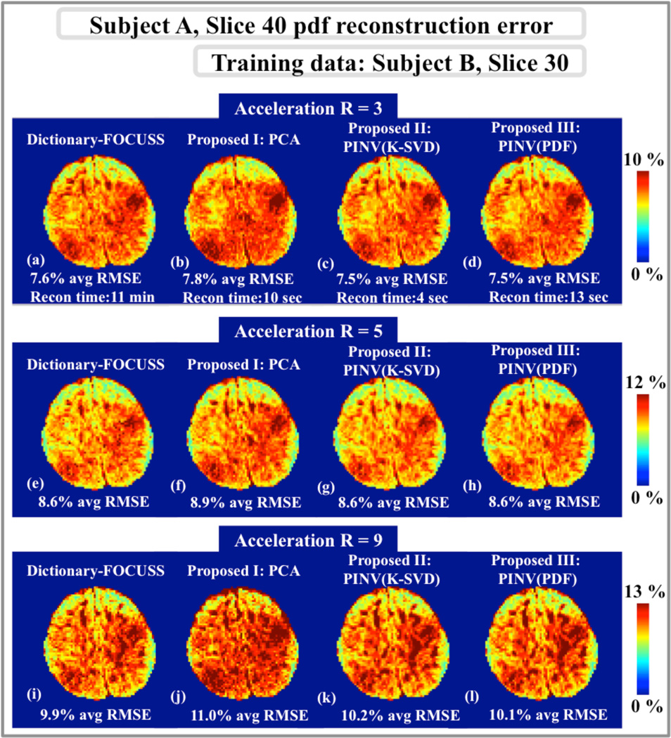
First, voxels in slice 40 of subject A were retrospectively undersampled in q-space, and reconstructed using all methods under consideration: Dictionary-FOCUSS, PCA, Tikhonov regularization with K-SVD dictionary (PINV(K-SVD)) and with training dataset itself as the dictionary (PINV(PDF)). The training data were sampled from slice 30 of subject B.
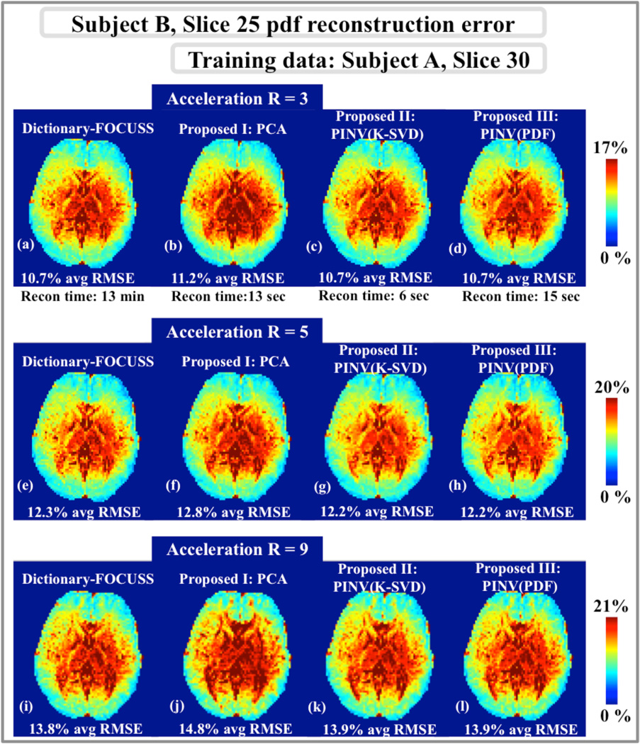
Second, voxels in slice 25 of subject B were retrospectively undersampled, and again reconstructed with Dictionary-FOCUSS, PCA, PINV(K-SVD) and PINV(PDF). In this experiment, the training data were obtained from slice 30 of subject A.
In these experiments, slice 30 was selected for training, and slices 25 and 40 were chosen for test based on their anatomical location, so that the test slices would reside on lower and upper parts of the brain, while the training slice was one of the middle slices. Three different acceleration factors, R=3, 5, and 9 were applied for dictionary-based reconstruction. By taking the fully-sampled data as ground-truth, the fidelity of the reconstruction methods were compared using root-mean-square error (RMSE) normalized by the ℓ2-norm of ground-truth as the error metric both in pdf domain and q-space.
The performance of K-SVD-trained dictionaries was evaluated for a range of training parameters ε (consistency constraint), s (sparsity level) and K (dictionary size). The lowest error was obtained with sparsity-constrained training at sparsity level s=10 and dictionary size K=258. All subsequent PINV(K-SVD) and Dictionary-FOCUSS reconstructions in the current work employed this “optimal” dictionary. Testing Dictionary-FOCUSS reconstruction error for various iteration number settings revealed that 5 outer loops of reweighted ℓ2 updates with 30 inner iterations to solve Eq. 5 yielded equivalent results to the previously reported 10 outer and 50 inner loops in [12]. Another source of performance gain for Dictionary-FOCUSS was the smaller size of the optimal dictionary (258 columns) as opposed to the overcomplete 3191-column dictionary employed in [12]. The combined effect of reduced iteration number and smaller dictionary size yielded about 45-times speed up for Dictionary-FOCUSS compared to reported speed in [12], without degrading the reconstruction performance.
Tikhonov regularization parameter λ for PINV and the dimension of the PCA space T were determined using the training data. In particular, reconstruction experiments were performed on the training dataset with the same undersampling pattern used for the test dataset, and the parameter that yielded the lowest RMSE was selected as the optimal regularization parameter. For PINV(K-SVD), at all acceleration factors and for both of subjects A and B, λ=0.01 was seen to yield the lowest RMSE values on the training set. Regarding PINV(PDF), λ=0.03 was the optimal parameter for all acceleration factors on subject A. For subject B, lowest error at R=3 and 5 was obtained with λ=0.1, while the optimal setting was λ=0.03 at R=9. The optimal dimension of the PCA space for subject A was found to be T=(50, 26, 22) at accelerations R=(3, 5, 9), respectively. For subject B, the corresponding values were T=(45, 27, 13).
To map the performance of the methods across the brain, reconstruction experiments on multiple slices across the whole brain were performed using Dictionary-FOCUSS, PCA, PINV(K-SVD), and PINV(PDF). Mean and standard deviation of RMSE in pdf domain for each slice were computed for subjects A and B.
In order to explore whether dictionary reconstruction generalizes across subjects, slice 40 of subject A was reconstructed using Dictionary-FOCUSS, PCA, PINV(K-SVD), and PINV(PDF) with dictionaries trained on data from subjects A, B, and C at R=3.
Since the fully-sampled data are corrupted by noise, computing RMSEs relative to them will include contributions from both reconstruction errors and additive noise. To address this, the additional 10 average data acquired at the selected five q-space points were used. As a single average full-brain DSI scan takes ~50 min, it was not practical to collect 10 averages for all of the undersampled q-space points. As such, we rely on both error metrics, namely: the RMSE relative to 1 average fully-sampled dataset and the RMSE relative to gold standard data for five q-space points.
To investigate how reconstruction error varies as a function of q-space location, at R=3, q-space images at the “missing” (not sampled) directions were computed using the pdfs estimated by all methods under consideration. RMSE values were obtained for all missing q-space directions by taking the fully-sampled 1 average dataset as ground truth.
Odf visualizations for a region of interest selected on slice 40 of subject A were computed for all methods at 3-fold undersampling. Additionally, fiber tractography solutions were computed for PCA, PINV(K-SVD) and PINV(PDF) reconstructions at 3-fold acceleration and for the fully-sampled dataset. We compared the images of a single subject, reconstructed from data using each of the three proposed reconstruction methods or reconstructed from fully sampled data, in terms of the tractography solutions that they produced. Streamline deterministic DSI tractography was performed on each data set in trackvis (http://trackvis.org) and 18 white-matter pathways were labeled. The labeling was performed following the protocol described in [31], where two regions of interest (ROIs) are drawn for each pathway in parts of the anatomy that the pathway is known to traverse. To eliminate variability due to manual labeling in the two data sets and make our comparison as unbiased as possible, the ROIs used here were not drawn manually on the each data set. Instead we obtained the ROIs from a different data set of 33 healthy subjects, where we had previously labeled the same pathways [32]. We averaged the respective ROIs from the 33 subjects in MNI space [33] and performed affine registration to map the average ROIs to the native space of each of the four data sets (fully sampled or 3-fold accelerated with the three proposed reconstruction methods). In each of the four data sets, we identified the tractography streamlines that went through the ROIs corresponding to each of the 18 pathways.
Results
Dictionary-FOCUSS, PCA, PINV(K-SVD), and PINV(PDF) reconstruction errors relative to fully-sampled pdfs in slice 40 of subject A are presented in Fig.1. All dictionary-based methods use the same training pdfs that were collected from slice 30 of subject B. At acceleration factor R=3, Dictionary-FOCUSS, PCA, PINV(K-SVD), and PINV(PDF) had 7.6%, 7.8%, 7.5%, and 7.5% average error, respectively. At the higher acceleration factor of R=5, Dictionary-FOCUSS, PCA, PINV(K-SVD), and PINV(PDF) yielded 8.6%, 8.9%, 8.6%, and 8.6% RMSE, respectively. At R=9, the average RMSE figures were 9.9%, 11.0%, 10.2%, and 10.1% for Dictionary-FOCUSS, PCA, PINV(K-SVD), and PINV(PDF). The computation times were 11 min for Dictionary-FOCUSS, 10 sec for PCA, 4 sec for PINV(K-SVD), and 13 sec for PINV(PDF).
Fig.1.
Pdf reconstruction error maps for slice 40 of subject A. a, b, c and d: At acceleration R=3, Dictionary-FOCUSS yielded 7.6% error in 11 min, PCA method resulted in 7.8% RMSE in 10 sec, PINV(K-SVD) had 7.5% error in 4 sec, and PINV(PDF) gave 7.5% error in 13 sec. e, f, g and h: At R=5, the dictionary-based methods yielded 8.6%, 8.9%, 8.6%, and 8.6% RMSE. i, j, k and l: At R=9, the reconstruction errors were 9.9%, 11.0%, 10.2%, and 10.1% for Dictionary-FOCUSS, PCA, PINV(K-SVD), and PINV(PDF), respectively.
Fig.2 compares pdf reconstruction errors obtained with the reconstruction methods under consideration for slice 25 of subject B. The training data for the dictionary-based methods were the pdfs in slice 30 of subject A. At acceleration R=3, Dictionary-FOCUSS, PCA, PINV(K-SVD), and PINV(PDF) returned 10.7%, 11.2%, 10.7%, and 10.7% average RMSE, respectively. At the higher acceleration factor of R=5, Dictionary-FOCUSS, PCA, PINV(K-SVD), and PINV(PDF) yielded 12.3%, 12.8%, 12.2%, and 12.2% RMSE, respectively. At R=9, the errors were 13.8%, 14.8%, 13.9%, and 13.9% for Dictionary-FOCUSS, PCA, PINV(K-SVD), and PINV(PDF). The computation times were 13 min for Dictionary-FOCUSS, 13 sec for PCA, 6 sec for PINV(K-SVD), and 15 sec for PINV(PDF).
Fig.2.
Pdf reconstruction error maps for slice 25 of subject B. a, b, c and d: At acceleration R=3, Dictionary-FOCUSS yielded 10.7% error in 13 min, the PCA method resulted in 11.2% error in 13 sec, PINV(K-SVD) had 10.7% RMSE in 6 sec, and PINV(PDF) obtained 10.7% error in 15 sec. e, f, g and h: At R=5, the four dictionary-based methods yielded 12.3%, 12.8%, 12.2%, and 12.2% RMSE. i, j, k and l: At R=9, the reconstruction errors were 13.8%, 14.8%, 13.9%, and 13.9% for Dictionary-FOCUSS, PCA, PINV(K-SVD), and PINV(PDF), respectively.
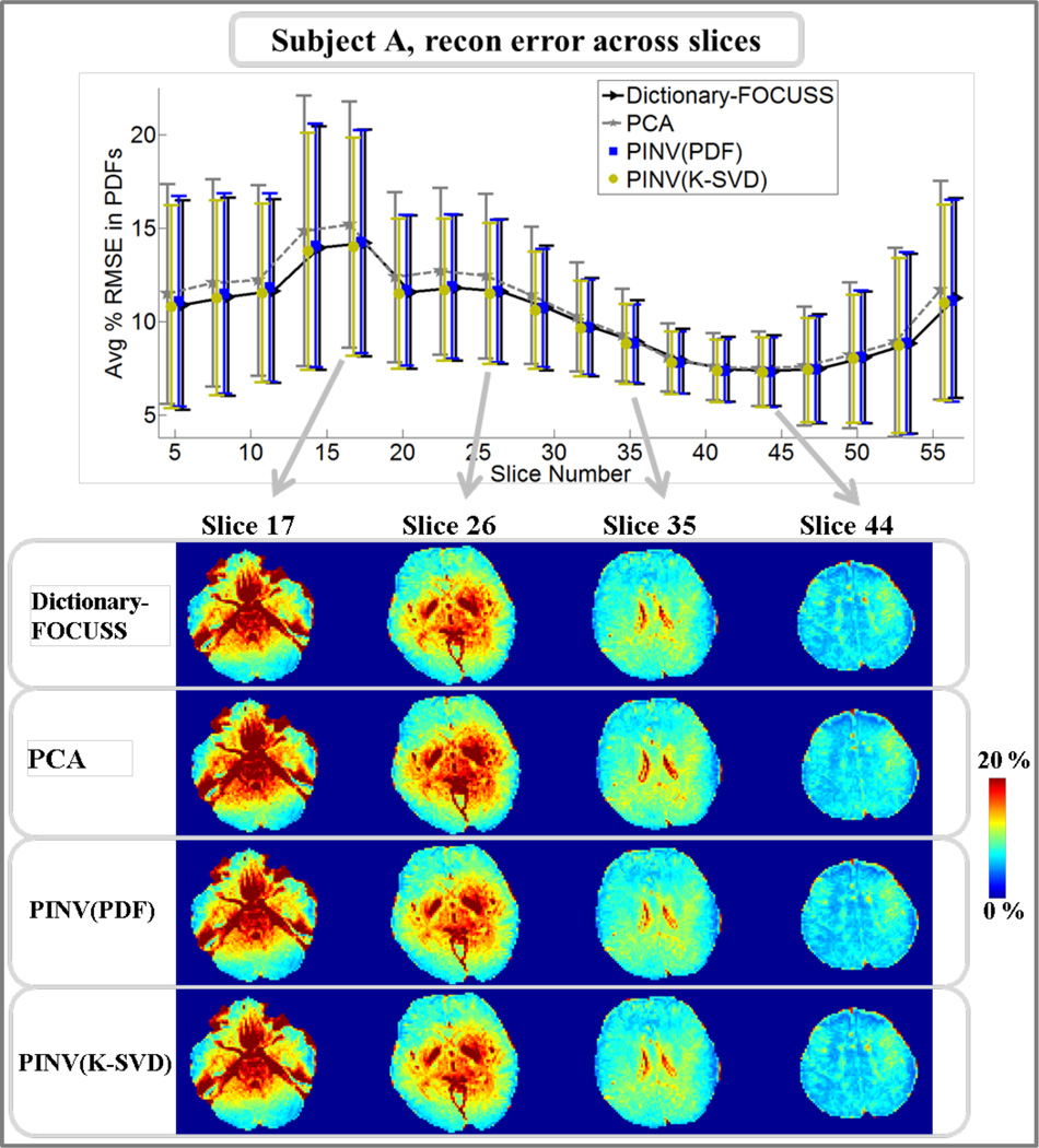
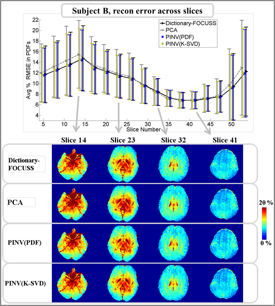
Pdf reconstruction errors for subject A across slices are plotted for Dictionary-FOCUSS, PCA, PINV(K-SVD), and PINV(PDF) in Fig.3. At four slices, RMSE maps are also depicted for comparison. The mean RMSE averaged across all slices was found to be 10.2% for Dictionary-FOCUSS, 10.8% for PCA, 10.1% for PINV(K-SVD), and 10.3% for PINV(PDF). Results from the same analysis are presented in Fig.4 for subject B. In this case, the mean RMSE averaged across all slices was found to be 10.2% for Dictionary-FOCUSS, 10.5% for PCA, 10.1% for PINV(K-SVD), and 10.1% for PINV(PDF).
Fig.3.
Upper panel: average and standard deviation of pdf reconstruction errors in each slice for subject A. Lower panel: comparison of Dictionary-FOCUSS, PCA, PINV(PDF), and PINV(K-SVD) error maps at four different slices.
Fig.4.
Upper panel: average and standard deviation of pdf reconstruction errors in each slice for subject B. Lower panel: comparison of Dictionary-FOCUSS, PCA, PINV(PDF), and PINV(K-SVD) error maps at four different slices.
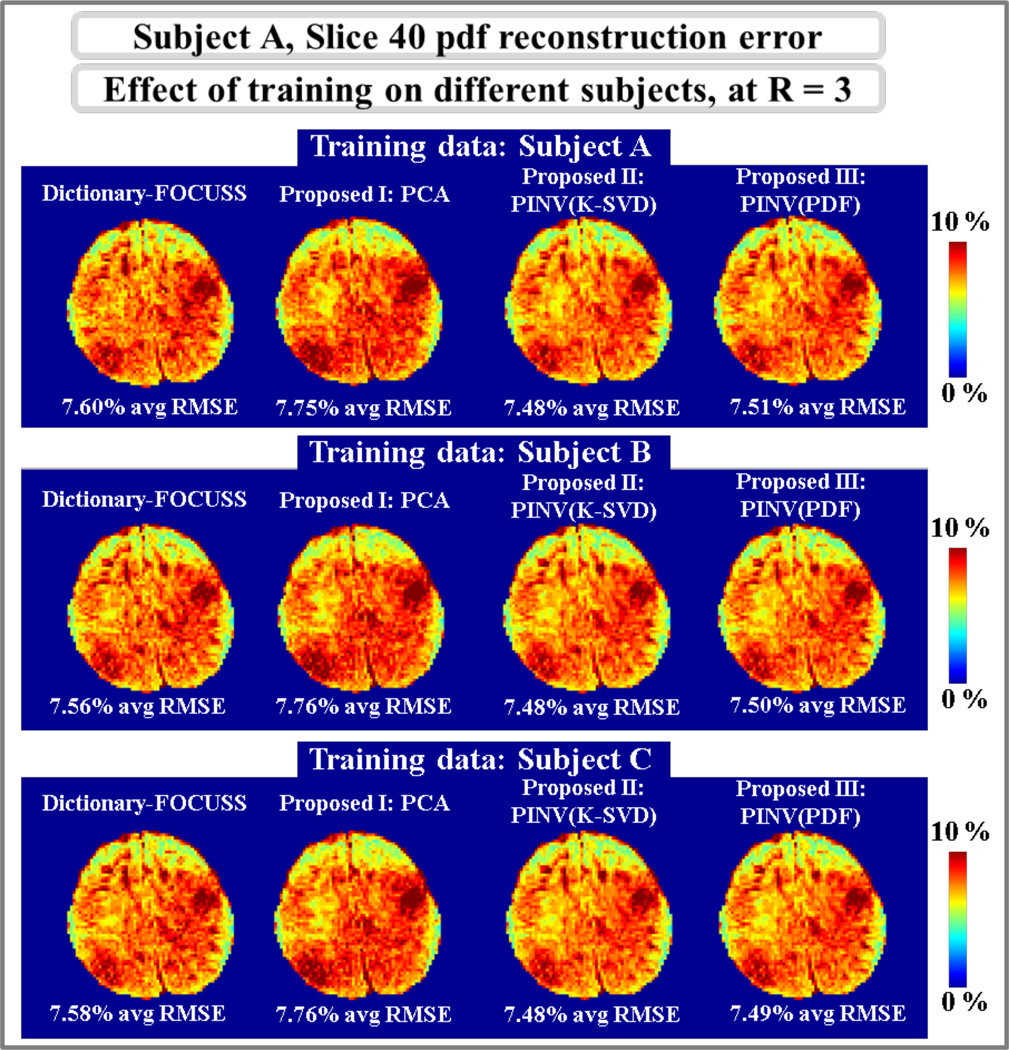
Using training data obtained from three different subjects, A, B and C, dictionary-based reconstruction at R=3 undersampling was performed on slice 40 of subject A. The resulting error maps are depicted in Fig.5, where Dictionary-FOCUSS had 7.60%, 7.56%, and 7.58% average RMSE with dictionaries trained on subjects A, B, and C, respectively. The mean errors were 7.75%, 7.76%, and 7.76% for PCA, 7.48% with all dictionaries for PINV(K-SVD) and 7.51%, 7.50%, and 7.49% for PINV(PDF) using training data from subjects A, B, and C.
Fig.5.
Top row: Reconstruction error maps of dictionary-based methods with training data from subject A. Middle row: training data from subject B. Bottom row: training data from subject C.
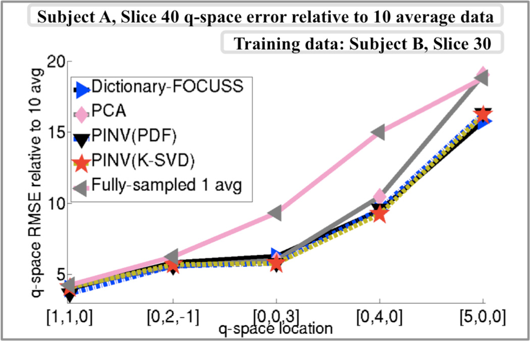
To isolate the reconstruction error from the contribution of noise to the RMSE figures, comparison against the 10 average dataset collected at 5 different q-space points is presented in Fig.6. The comparison is based on slice 40 of subject A at 3-fold undersampling, while the data used for dictionary training were slice 30 of subject B. The average error for each of the curves in Fig.6 were 10.7% for fully-sampled 1 average data, 8.3% for Dictionary-FOCUSS, 9.0% for PCA, 8.2% for PINV(K-SVD), and 8.2% for PINV(PDF) reconstruction.
Fig.6.
q-space reconstruction errors relative to the 10 average data collected in five q-locations. On average, the RMSE figures were 10.7% for 1 average fully-sampled data, 8.3% for Dictionary-FOCUSS, 9.0% for PCA, 8.2% for PINV(K-SVD) and 8.2% for PI NV(PDF).
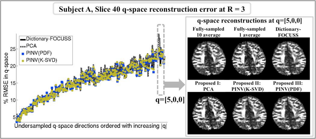
Reconstruction errors at acceleration R=3 for slice 40 of subject A at the “missing” q-space points are plotted in Fig.7. When averaged over all missing q-space points, the RMSEs were found to be 15.5% for Dictionary-FOCUSS, 15.8% for PCA, 15.4% for PINV(K-SVD), and 15.4% for PINV(PDF). The panel on the right shows the q-space images at the location [5,0,0] estimated by the six reconstruction methods, as well as the fully-sampled 10 average and 1 average images.
Fig.7.
Left: q-space reconstruction errors at the missing directions relative to the 1 average fully sampled data. When averaged over the missing q-space points, the RMSEs were found to be 15.5% for Dictionary-FOCUSS, 15.8% for PCA, 15.4% for PINV(K-SVD), and 15.4% for PINV(PDF). Right: q-space reconstructions at the point q=[5,0,0].
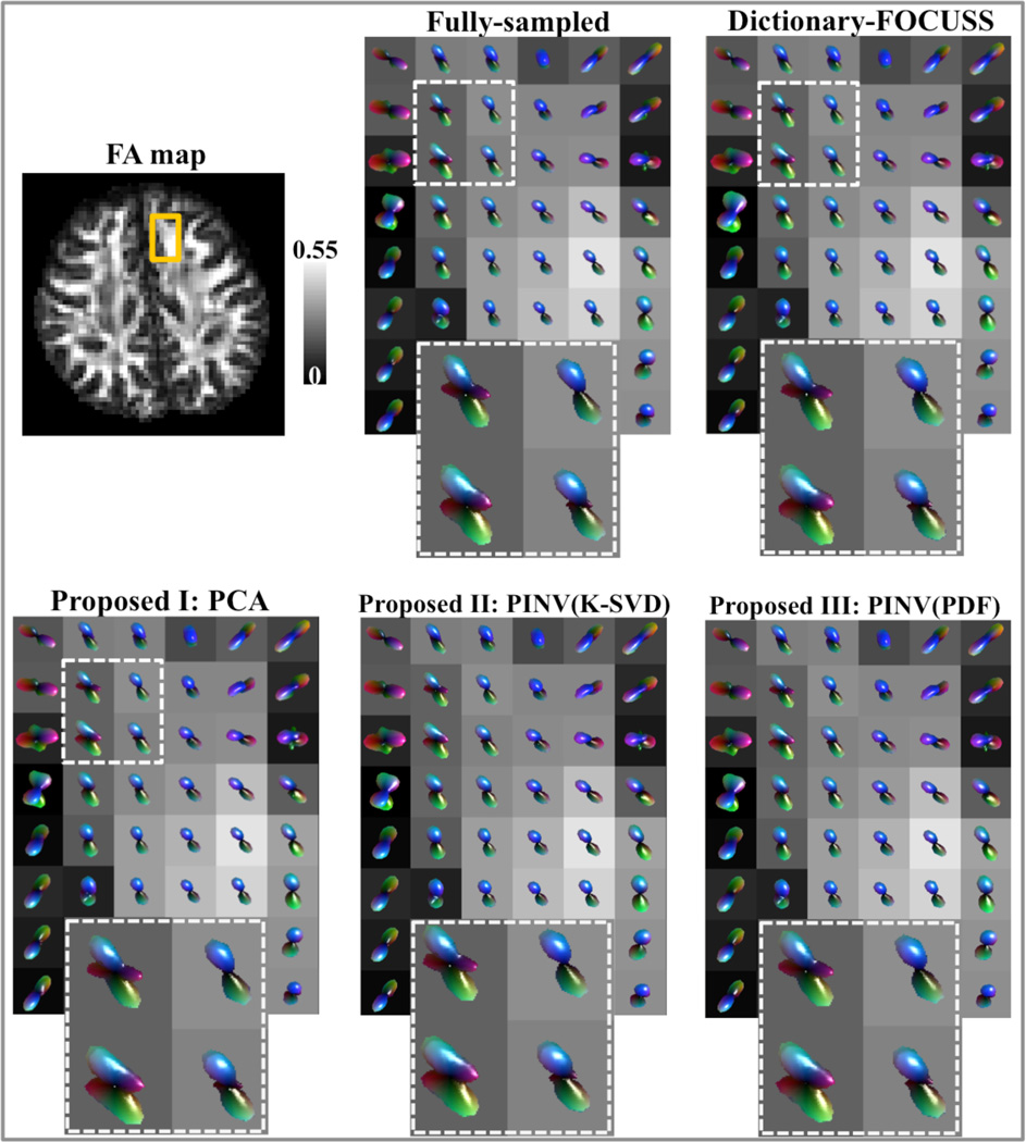
Odf visualizations based on the pdfs reconstructed by the four methods at 3-fold acceleration are compared with the glyphs obtained from the fully-sampled data for slice 40 of subject A in Fig.8. The region of interest is marked on the Fractional Anisotropy (FA) map, inside which four voxels are further magnified.
Fig.8.
Odf visualizations at R=3 for Dictionary-FOCUSS, PCA, PINV(K-SVD), and PINV(PDF) are compared against the glyphs obtained with fully-sampled data.
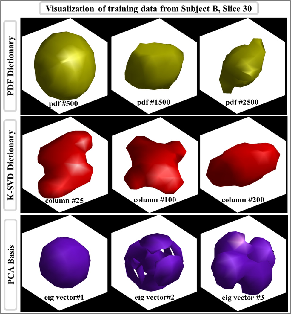
Isosurface plots for three example pdfs from the pdf training dataset, three columns from the 258-column K-SVD dictionary, and the first three eigenvectors in the PCA-basis are depicted in Fig.9. For each plot in PDF and K-SVD dictionaries, the isosurface level was determined to be at 5% of the maximum value in the column vector. For the PCA eigenvectors, isosurface was computed at 20% of the maximum value in each vector.
Fig.9.
Isosurface plots of PDF, K-SVD, and PCA based dictionary columns obtained from slice 30 of subject B.
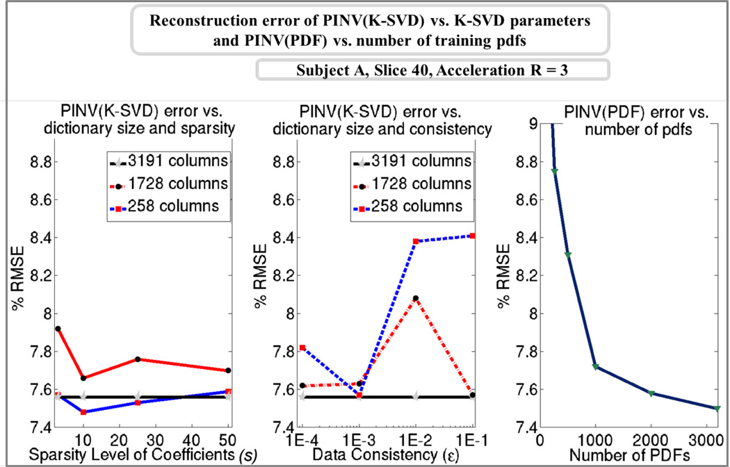
The dependence of K-SVD based Tikhonov-regularized reconstruction PINV(K-SVD) on the K-SVD training parameters ε (data consistency constraint), s (sparsity level), and K (the number of dictionary columns) is explored in Fig.10. For sparsity-based training, transform coefficients with at most s = (3, 10, 25, 50) non-zero elements were considered. With data consistency-based K-SVD training, consistency levels of ε = (10−4, 10−3, 10−2, 10−1) were employed. In both cases, three dictionary sizes were used. K = 258 corresponds to the rank of the real part of the pdf training set P used in generating the K-SVD dictionaries. K = 1728 is equal to the dimension of the pdf signals, and yields a square-sized dictionary. K = 3191 is the number of training pdf samples, which allows an overcomplete representation. Among the 24 K-SVD dictionaries, sparsity-based training with K = 258 columns and s = 10 elements gave the smallest error of 7.48% while reconstructing slice 40 of subject A at 3-fold acceleration. This parameter setting was chosen to be optimal one and was used in all results reported with Dictionary-FOCUSS and PINV(K-SVD). Additionally, Fig.10 investigates the reconstruction performance of PINV(PDF) as a function of the number of pdfs in the training dataset. The lowest error of 7.50% was obtained when all 3191 pdfs were included in the PDF dictionary.
Fig.10.
Left: Error of sparsity-based K-SVD trained dictionary reconstruction for different dictionary sizes and sparsity levels. Middle: Error of consistency-based trained dictionary reconstruction as a function of dictionary size and data consistency constraint. Right: Dependence of PINV(PDF) performance on the amount of pdfs included in the PDF dictionary.
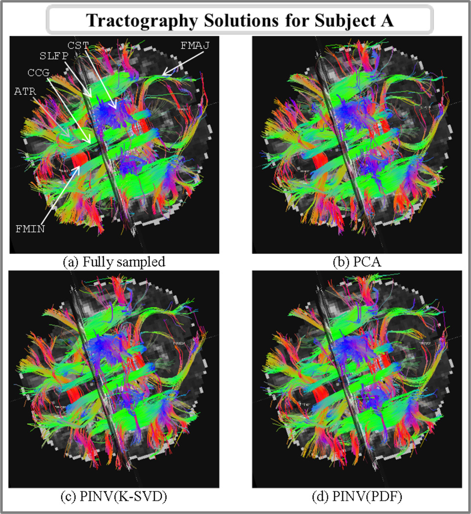
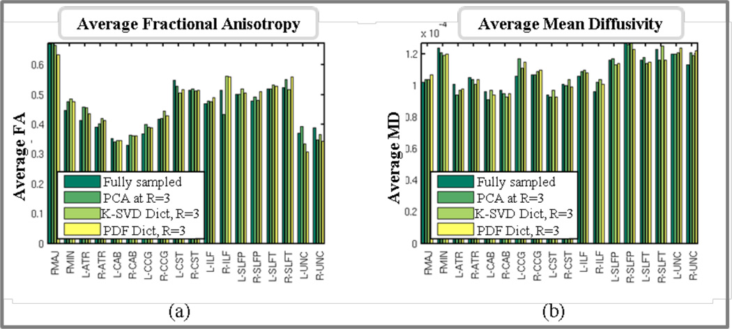
Fig. 11 shows the tractography solutions of subject A in the fully sampled and 3-fold accelerated reconstructions using the PCA, PINV(K-SVD) and PINV(PDF) methods. Fig. 12 shows plots of the average fractional anisotropy (FA) and mean diffusivity (MD) of each of the 18 white-matter pathways, as calculated from each of these four reconstructions.
Fig.11.
Axial view of white-matter pathways labeled from streamline DSI tractography in fully sampled data and 3-fold accelerated data reconstructed with PCA, PINV(K-SVD) and PINV(PDF). The following pathways are visible in this view: corpus callosum - forceps minor (FMIN), corpus callosum - forceps major (FMAJ), anterior thalamic radiations (ATR), cingulum - cingulate gyrus bundle (CCG), superior longitudinal fasciculus - parietal bundle (SLFP), and the superior endings of the corticospinal tract (CST).
Fig.12.
Average FA (left) and MD (right) for each of the 18 labeled pathways, as obtained from the fully sampled data and 3-fold accelerated data reconstructed with PCA, PINV(K-SVD) and PINV(PDF). Intra-hemispheric pathways are indicated by “L-” (left) or “R-” (right). The pathways are: corpus callosum - forceps major (FMAJ), corpus callosum - forceps minor (FMIN), anterior thalamic radiation (ATR), cingulum - angular (infracallosal) bundle (CAB), cingulum - cingulate gyrus (supracallosal) bundle (CCG), corticospinal tract (CST), inferior longitudinal fasciculus (ILF), superior longitudinal fasciculus - parietal bundle (SLFP), superior longitudinal fasciculus - temporal bundle (SLFT), uncinate fasciculus (UNC).
Discussion
The three proposed methods PINV(K-SVD), PINV(PDF), and PCA were demonstrated to have reconstruction quality comparable to that of Dictionary-FOCUSS in pdf and odf domains and q-space based on Figs. 1 through 8. At the same time, they attained 2 orders of magnitude reduction in computation time relative to Dictionary-FOCUSS. With this initial implementation, which reconstructs an entire slice at once and runs on Matlab, processing times as low as 5 seconds per slice are already achievable. While being feasible for clinical application of accelerated DSI, the presented methods do not sacrifice reconstruction quality for computation speed.
The governing idea of this work is that the key to good reconstruction quality is the priors encoded in a dictionary, and not the particular type regularization applied on the transform coefficients. Constraining the reconstructed pdfs to be a linear combination of the dictionary columns is shown to be a much stronger prior than sparsity or smoothness constraints on the linear combination weights. As such, simple ℓ2-regularized reconstruction yields as good results as the iterative ℓ1 solution, as long as a dictionary is involved. Indeed, using the same dictionary made of 258 columns that requires at most 10 dictionary columns to represent the training dataset, Dictionary-FOCUSS with ℓ1-regularization, and PINV(K-SVD) with ℓ2-constraint yield very similar results. To further support the claim that sparsity is not essential, we proposed PCA and PINV(PDF) methods that include no sparsity assumption in either training or reconstruction steps. In fact, PINV(PDF) is so simple that it only requires the reconstructed pdfs to be in the range of training pdfs, but it works equally well as the other more involved methods presented in this work. The advantage of using a K-SVD trained dictionary is that it allows a more compact representation, while a couple of thousand pdfs are required to achieve good reconstruction quality in PINV(PDF) (Fig.10). To show that K-SVD trained 258-column dictionary and the 3191-column dictionary made from training pdfs have equivalent representation power, we computed the difference in the range of these dictionaries via,
| Eq.20 |
Here, residual is the energy of the part of one dictionary that cannot be represented by the other one. To arrive at this relation, note that left singular vectors corresponding to the non-zero singular values of a matrix span the range of this matrix. By applying SVD on the K-SVD trained dictionary and the dictionary made of training pdfs and keeping the 258 columns corresponding to the significant singular values, the matrices G and H that span the range of these two dictionaries are obtained. The expression (GGH − I)H then gives the difference between the span of one dictionary and its projection onto the range of the other. For K-SVD and PDF dictionaries, residual was computed to be 8.9·10−12, which is negligibly small. As such, PINV(PDF) method by-passes sparsity assumptions and dictionary training without compromising representative power.
To further support the point that the presence of a dictionary that represents the pdfs is essential, we set the dictionary in PINV reconstruction to the identity matrix I, so that ℓ2-penalty is applied on the pdfs themselves, rather than dictionary transform coefficients. At 3-fold acceleration, this resulted in a substantially high error of 68.6% for slice 40 of subject A. Moreover, if ℓ1-regularization is applied on the pdfs by setting the dictionary to the identity matrix I in the FOCUSS algorithm, 15.6% RMSE is obtained. In contrast, using a pdf-based dictionary with PINV(PDF) reduced this error 7.5% (Fig.1).
An alternative approach to improving reconstruction speed is to increase the convergence rate of iterative CS algorithms through Nesterov-type gradient descent algorithms [34]. These optimal methods rely on a weighted combination of all previous gradients, and reduce the number of iterations required to reach a certain solution precision. With the FISTA algorithm [34], wavelet-based deblurring was seen to require 10 times fewer number of iterations compared to gradient descent. However, even with optimal descent techniques, processing time of CS algorithms would still remain above an hour for full brain reconstruction, which may not be a clinically feasible interval. Further, ℓ1 regularization parameters need to be determined for such optimal CS algorithms. Parallel programming and optimized implementation in an efficient language such as C++ are two potential sources of performance gain for all methods considered in the current work.
For all of the proposed methods, there is also one parameter that needs to be tuned, namely, the ℓ2 regularization parameter for PINV(K-SVD) and PINV(PDF), and the number of columns kept in PCA. We propose to use the fully-sampled training dataset to determine “optimal” parameters with respect to the RMSE metric. Using the same undersampling pattern that will be applied on the test dataset, the parameter setting that yields the lowest reconstruction RMSE on the training dataset is determined by parameter sweeping. We note that there are other established ways to determine these regularization parameters (e.g., L-curve method [25], cross-validation). With the assumption that fully-sampled data exist for dictionary training, we further utilized this set for parameter extraction. For subject A, the dimension of the PCA space was determined by minimizing the reconstruction error on the training set from subject B to obtain the optimal values T=(50, 26, 22) at R=(3, 5, 9). Instead, if the parameters were determined by optimizing the performance on subject A, the optimal values would be T=(49, 24, 23). This set of parameters would yield 7.7%, 8.9% and 10.9% at R=(3, 5, 9), compared to 7.8%, 8.9%, and 11.0% obtained in Fig.1 with the parameters determined on the training set. The difference is mild, causing a change of at most 0.1% in the average error.
Similarly for subject B, the optimal parameter setting was found to be T=(45, 27, 13) based on the training dataset from subject A. Assuming that it was possible to optimize the parameters with data from subject B, T=(45, 22, 13) would have been obtained. In this case, the only difference is at R=5, where the RMSE in Fig.2h would decrease from 12.8% to 12.6% if T=22 was used instead of T=27. Hence, the PCA parameters extracted from the training dataset generalize very well to the test dataset and yield close to optimal reconstruction performance.
Because the optimal PCA dimension was seen to differ across subjects (for A, T=(50, 26, 22) and for B, T=(45, 27, 13)), we tested the effect of applying the optimal T determined for subject A while reconstructing B and vice versa. Regarding slice 40 of subject A, the error values became 7.7%, 9.0% and 11.5% at R=(3, 5, 9), compared to 7.8%, 8.9% and 11.0% RMSE in Fig.1. Regarding the reconstruction of slice 25 of subject B, the RMSEs would change to 11.5%, 12.8%, and 15.8% at R=(3, 5, 9) compared to 11.2%, 12.8% and 14.8% obtained in Fig.2. These results suggest that optimal number of columns for PCA reconstruction generalizes across subjects, except when very high acceleration factors are employed.
The number of PCA columns that yielded the lowest error was seen to decrease as the acceleration factor increased. PCA reconstruction in Eq.15 involves the solution of a least squares problem via the pseudoinverse of FΩQT, and this problem is ill-conditioned if the condition number of FΩQT is large. In this case, small errors in the entries of this matrix can lead to large errors in the solution vector. While keeping the number of columns T fixed, it was observed that the condition number increased as the acceleration factor increased. For instance, letting T=100, cond (FΩQT) was computed to be 6.8 at R=3, 113.2 at R=5, and 2.0·1014 at R=9. This indicates that smaller number of columns needs to be used at higher accelerations to keep the least squares problem well-conditioned.
The regularization parameter λ for PINV(K-SVD) and PINV(PDF) was seen to be relatively insensitive to changes in the acceleration factor R. For reconstruction of subject A, the optimal parameters were determined on the training dataset from subject B, and were found to be λ=10−2 for PINV(K-SVD) and λ=3·10−2 for PINV(PDF) for all undersampling factors. If the optimal parameters were determined on the test data itself, λ=10−2 for PINV(K-SVD) and λ=3·10−2 for PINV(PDF) would again be obtained at R = 3 and 5. However, slightly lower regularization parameters of λ=3·10−3 and λ=10−2 would be obtained at R = 9. Regarding subject B, the optimal parameters determined on the training dataset were λ=10−2 for PINV(K-SVD) and λ=10−1 for PINV(PDF) at all acceleration factors, except that λ=3·10−2 at R = 9 was chosen for PINV(PDF). If these parameters were determined on the test data itself, λ=10−2 for PINV(K-SVD) and λ=10−1 for PINV(PDF) at all R factors would be selected. Based on this analysis, the regularization parameters selected on the fully-sampled training dataset are seen to generalize well to reconstruction of undersampled test data. These parameters are also insensitive to the acceleration factor employed, further increasing the robustness of the proposed Tikhonov-regularized methods.
To explore whether dictionary-based methods generalize across healthy subjects, dictionaries trained on three different subjects were employed in reconstruction of a single slice from subject A. For all of the dictionary-based methods, essentially the same RMSE values were obtained with data from each subject (Fig.5). While this indicates that the proposed methods generalize well among young and healthy subjects, it remains an open question whether the same observation can be made across different age groups or patient populations. The impact of using different imaging parameters on generalization of dictionary reconstruction also warrants further investigation. It is especially likely that employing different scan parameters would cause the pdf shapes to change, as this would correspond to a different snapshot of the diffusion process.
When 10 average data were taken as ground truth (Fig.6), all four dictionary-based methods at 3-fold acceleration were seen to yield lower error than the fully-sampled 1 average data. This could indicate that dictionary-based techniques successfully estimate the missing q-space samples as well as denoise the q-space. In accordance with this conclusion, K-SVD was recently proposed as a denoising tool for high-angular diffusion imaging (HARDI) [35], where training and denoising were performed on q-space images.
Regarding the PCA method, using a lower dimensional space reduces the number of coefficients that need to be estimated from the sampled q-space points. Considering the case at R=3 with T=50 principal components, the projected pdfs reside in a 50-dimensional space whose coordinates need to be determined using 171 q-space samples (at 3-fold undersampling for 515 directions). Rather than operating in the pdf space with 12×12×12 = 1728 dimensions, PCA method seeks 50 coefficients, thus substantially reduces the effective undersampling factor of the problem. This is thanks to the prior information encoded in the training pdf dataset.
Optimization of the dictionary trained with the K-SVD algorithm with respect to the training parameters was investigated in Fig.10. The lowest RMSE of 7.48% was obtained with the smallest dictionary of column size K=258 at the sparsity level s=10. However, the performance is relatively insensitive to the training parameters, e.g. 7.56% RMSE is obtained with the overcomplete dictionary at any sparsity or consistency level. The reason why the overcomplete dictionary remains the same while the parameters change is that, it is possible to represent any training pdf using a single dictionary coefficient, as the number of columns is equal to the number of training pdfs. Hence, using an overcomplete dictionary would simplify the parameter selection in K-SVD training while remaining close to optimal in terms of reconstruction quality. The Dictionary-FOCUSS results reported in [12] were all obtained with overcomplete dictionaries. This selection substantially increases the reconstruction times, since the overcomplete dictionary is about 10 times larger than the optimal 258-column dictionary employed here. By reducing the number of iterations about 3 times and the dictionary size about 12 times, we were able to obtain 45-times speed up in Dictionary-FOCUSS reconstruction relative to [12], without degrading the RMSE values. Still, the proposed methods are two orders of magnitude faster than this newly optimized version of Dictionary-FOCUSS reconstruction.
Rather than matching the q-space data with equality, it is possible to formulate FOCUSS reconstruction in Eq.5 as an unconstrained optimization problem [36] as follows,
| Eq.21 |
Via the mapping x = Ws, this update step would result in ℓ1-regularized reconstruction,
| Eq.22 |
where γ is a regularization parameter that needs to be determined. At R=3 on slice 40 of subject A, equality constrained reconstruction yielded 7.56% RMSE. With parameter sweeping, the optimal γ was found to be 10−4, with an error of 7.54%. Since the improvement in performance is negligible and the parameter γ needs to be tuned, regularized version of FOCUSS was not used in this work.
In addition to comparison in pdf domain and q-space as well as validation with respect to low-noise 10 average dataset, reconstruction methods were also compared against the fully-sampled acquisition in terms of fidelity in odf reconstruction and fiber tractography. Fig.8 demonstrates good correspondence between the fully-sampled odfs and all four dictionary-based methods at 3-fold undersampling.
Example atoms from PDF, K-SVD and PCA based dictionaries are plotted in Fig.9. Top row depicts iso-probability surfaces for three individual pdfs that were sampled from Subject B. In the middle row, three columns of K-SVD-trained dictionary are reformatted to the three-dimensional grid for display purposes. The final row shows the first three eigenvectors of the PCA representation. As opposed to the K-SVD atoms, the columns of the PCA basis do not resemble individual pdfs, since they represent the principal components of the training dataset. These eigenvectors summarize the variance in the dataset within a small number dimensions, hence they are not visually similar to the pdf isosurfaces plotted in the top row.
Visual inspection of the tractography solutions (Fig. 11) showed that similar white-matter pathways could be obtained from the images reconstructed from the fully sampled data and the 3-fold accelerated data with PCA, PINV(K-SVD) and PINV(PDF). The mean Hausdorff distance between the pathways obtained from the fully sampled reconstruction and each of the accelerated reconstructions, averaged over all 18 pathways was 3.2mm for PCA and 4.5mm for both PINV(K-SVD) and PINV(PDF). This is less than 2 voxels, which we have previously found to be the inter-rater test-retest reliability of manually labeling the pathways [32].
We also found good agreement between the average FA and MD values in the four data sets (Fig. 12). The mean difference between the average FA values in the fully sampled and 3-fold accelerated reconstructions, as a percentage of the value in the fully sampled data, was 5.0%, 5.2%, and 6.0%, respectively, for the PCA, PINV(K-SVD), and PINV(PDF) reconstructions. The same errors for the average MD values were, respectively, 3.2%, 3.1%, and 3.4%.
Conclusion
To accelerate the acquisition speed of DSI, two dictionary-based reconstruction algorithms that estimate diffusion pdfs from undersampled q-space were proposed. Using the same training data, these methods decrease the computation time by 2 orders of magnitude relative to dictionary-based compressed sensing algorithm [12], making the use of such algorithms feasible for clinical applications. Experiments on in vivo data show that the proposed algorithms yield comparable reconstruction quality to that of dictionary-based CS in terms of pdf, odf and tractrography solutions. The proposed methods do not make sparsity assumptions on the reconstructed pdfs, instead constrain them to be a linear combination of the dictionary columns. These fast ℓ2-based algorithms also simplify the training step: dictionaries obtained with simple linear algebra operations or without any training perform equally well as the more involved K-SVD training. Further, it is demonstrated that a dictionary trained using pdfs from a single slice of a particular subject generalizes well to slices at different anatomical regions from another subject.
Acknowledgement
NIH R01 EB007942; NIBIB K99EB012107; NIBIB R01EB006847; K99/R00 EB008129; NCRR P41RR14075 and the NIH Blueprint for Neuroscience Research U01MH093765 The Human Connectome project; Siemens Healthcare; Siemens-MIT Alliance; MIT-CIMIT Medical Engineering Fellowship
References
- 1.Callaghan PT, Eccles CD, Xia Y. Nmr Microscopy of Dynamic Displacements - K-Space and Q-Space Imaging. Journal of Physics E-Scientific Instruments. 1988 Aug;21(8):820–822. [Google Scholar]
- 2.Wedeen VJ, Hagmann P, Tseng WY, Reese TG, Weisskoff RM. Mapping complex tissue architecture with diffusion spectrum magnetic resonance imaging. Magn Reson Med. 2005 Dec;54(6):1377–1386. doi: 10.1002/mrm.20642. [DOI] [PubMed] [Google Scholar]
- 3.Merlet S, Philippe AC, Deriche R, Descoteaux M. Tractography via the ensemble average propagator in diffusion MRI. Med Image Comput Comput Assist Interv. 2012;15(Pt 2):339–346. doi: 10.1007/978-3-642-33418-4_42. [DOI] [PubMed] [Google Scholar]
- 4.Larkman DJ, Hajnal JV, Herlihy AH, Coutts GA, Young IR, Ehnholm G. Use of multicoil arrays for separation of signal from multiple slices simultaneously excited. Journal of Magnetic Resonance Imaging. 2001 Feb;13(2):313–317. doi: 10.1002/1522-2586(200102)13:2<313::aid-jmri1045>3.0.co;2-w. [DOI] [PubMed] [Google Scholar]
- 5.Moeller S, Yacoub E, Olman CA, Auerbach E, Strupp J, Harel N, Ugurbil K. Multiband Multislice GE-EPI at 7 Tesla, With 16-Fold Acceleration Using Partial Parallel Imaging With Application to High Spatial and Temporal Whole-Brain FMRI. Magnetic Resonance in Medicine. 2010 May;63(5):1144–1153. doi: 10.1002/mrm.22361. [DOI] [PMC free article] [PubMed] [Google Scholar]
- 6.Setsompop K, Cohen-Adad J, Gagoski BA, Raij T, Yendiki A, Keil B, Wedeen VJ, Wald LL. Improving diffusion MRI using simultaneous multi-slice echo planar imaging. Neuroimage. 2012 Oct 15;63(1):569–580. doi: 10.1016/j.neuroimage.2012.06.033. [DOI] [PMC free article] [PubMed] [Google Scholar]
- 7.Reese TG, Benner T, Wang R, Feinberg DA, Wedeen VJ. Halving Imaging Time of Whole Brain Diffusion Spectrum Imaging and Diffusion Tractography Using Simultaneous Image Refocusing in EPI. Journal of Magnetic Resonance Imaging. 2009 Mar;29(3):517–522. doi: 10.1002/jmri.21497. [DOI] [PMC free article] [PubMed] [Google Scholar]
- 8.Feinberg DA, Reese TG, Wedeen VJ. Simultaneous echo refocusing in EPI. Magn Reson Med. 2002 Jul;48(1):1–5. doi: 10.1002/mrm.10227. [DOI] [PubMed] [Google Scholar]
- 9.Feinberg DA, Moeller S, Smith SM, Auerbach E, Ramanna S, Glasser MF, Miller KL, Ugurbil K, Yacoub E. Multiplexed Echo Planar Imaging for Sub-Second Whole Brain FMRI and Fast Diffusion Imaging. PLoS One. 2010 Dec 20;5(12) doi: 10.1371/journal.pone.0015710. [DOI] [PMC free article] [PubMed] [Google Scholar]
- 10.Setsompop K, Gagoski BA, Polimeni JR, Witzel T, Wedeen VJ, Wald LL. Blipped-controlled aliasing in parallel imaging for simultaneous multislice echo planar imaging with reduced g-factor penalty. Magn Reson Med. 2012 May;67(5):1210–1224. doi: 10.1002/mrm.23097. [DOI] [PMC free article] [PubMed] [Google Scholar]
- 11.Menzel MI, Tan ET, Khare K, Sperl JI, King KF, Tao XD, Hardy CJ, Marinelli L. Accelerated Diffusion Spectrum Imaging in the Human Brain Using Compressed Sensing. Magnetic Resonance in Medicine. 2011 Nov;66(5):1226–1233. doi: 10.1002/mrm.23064. [DOI] [PubMed] [Google Scholar]
- 12.Bilgic B, Setsompop K, Cohen-Adad J, Yendiki A, Wald LL, Adalsteinsson E. Accelerated diffusion spectrum imaging with compressed sensing using adaptive dictionaries. Magn Reson Med. 2012 Dec;68(6):1747–1754. doi: 10.1002/mrm.24505. [DOI] [PMC free article] [PubMed] [Google Scholar]
- 13.Gorodnitsky IF, Rao BD. Sparse signal reconstruction from limited data using FOCUSS: A re-weighted minimum norm algorithm. Ieee Transactions on Signal Processing. 1997 Mar;45(3):600–616. [Google Scholar]
- 14.Aharon M, Elad M, Bruckstein A. K-SVD: An algorithm for designing overcomplete dictionaries for sparse representation. Ieee Transactions on Signal Processing. 2006 Nov;54(11):4311–4322. [Google Scholar]
- 15.Merlet SL, Paquette M, Deriche R, Descoteaux M. Ensemble Average Propagator Reconstruction via Compressed Sensing: Discrete or Continuous Bases?. 20th annual meeting of the International Society for Magnetic Resonance in Medicine; Melbourne, Australia. 2012. [Google Scholar]
- 16.Merlet S, Deriche RD. Compressed sensing for accelerated EAP recovery in diffusion MRI. CDMRI'10. 2010 [Google Scholar]
- 17.Lee N, Singh M. Compressed Sensing based Diffusion Spectrum Imaging. 18th Annual ISMRM Scientific Meeting and Exhibition 2010; Stockholm, Sweden. [Google Scholar]
- 18.Merlet S, Caruyer E, Deriche R. Parametric dictionary learning for modeling EAP and ODF in diffusion MRI. Med Image Comput Comput Assist Interv. 2012;15(Pt 3):10–17. doi: 10.1007/978-3-642-33454-2_2. [DOI] [PubMed] [Google Scholar]
- 19.Gramfort A, Poupon C, Descoteaux M. Sparse DSI: learning DSI structure for denoising and fast imaging. Med Image Comput Comput Assist Interv. 2012;15(Pt 2):288–296. doi: 10.1007/978-3-642-33418-4_36. [DOI] [PubMed] [Google Scholar]
- 20.Michailovich O, Rathi Y, Dolui S. Spatially regularized compressed sensing for high angular resolution diffusion imaging. IEEE Trans Med Imaging. 2011 May;30(5):1100–1115. doi: 10.1109/TMI.2011.2142189. [DOI] [PMC free article] [PubMed] [Google Scholar]
- 21.Tristan-Vega A, Westin CF. Probabilistic ODF estimation from reduced HARDI data with sparse regularization. Med Image Comput Comput Assist Interv. 2011;14(Pt 2):182–190. doi: 10.1007/978-3-642-23629-7_23. [DOI] [PMC free article] [PubMed] [Google Scholar]
- 22.Rathi Y, Michailovich O, Setsompop K, Bouix S, Shenton ME, Westin CF. Sparse multi-shell diffusion imaging. Med Image Comput Comput Assist Interv. 2011;14(Pt 2):58–65. doi: 10.1007/978-3-642-23629-7_8. [DOI] [PMC free article] [PubMed] [Google Scholar]
- 23.Miranda AA, Le Borgne YA, Bontempi G. New routes from minimal approximation error to principal components. Neural Processing Letters. 2008 Jun;27(3):197–207. [Google Scholar]
- 24.Hansen PC. The Truncated Svd as a Method for Regularization. Bit. 1987;27(4):534–553. [Google Scholar]
- 25.Hansen PC. The L-Curve and its Use in the Numerical Treatment of Inverse Problems. Computational inverse problems in electrocardiology. 2000:119–142. [Google Scholar]
- 26.Keil B, Blau JM, Hoecht P, Biber S, Hamm M, Wald LL. A 64-channel brain array coil for 3T imaging. 20th Annual ISMRM Scientific Meeting and Exhibition 2012; Melbourne, Australia. [Google Scholar]
- 27.Griswold MA, Jakob PM, Heidemann RM, Nittka M, Jellus V, Wang J, Kiefer B, Haase A. Generalized autocalibrating partially parallel acquisitions (GRAPPA) Magn Reson Med. 2002 Jun;47(6):1202–1210. doi: 10.1002/mrm.10171. [DOI] [PubMed] [Google Scholar]
- 28.Bodammer N, Kaufmann J, Kanowski M, Tempelmann C. Eddy current correction in diffusion-weighted imaging using pairs of images acquired with opposite diffusion gradient polarity. Magnetic Resonance in Medicine. 2004 Jan;51(1):188–193. doi: 10.1002/mrm.10690. [DOI] [PubMed] [Google Scholar]
- 29.Jenkinson M, Bannister P, Brady M, Smith S. Improved optimization for the robust and accurate linear registration and motion correction of brain images. Neuroimage. 2002 Oct;17(2):825–841. doi: 10.1016/s1053-8119(02)91132-8. [DOI] [PubMed] [Google Scholar]
- 30.Lustig M, Donoho D, Pauly JM. Sparse MRI: The application of compressed sensing for rapid MR imaging. Magn Reson Med. 2007 Dec;58(6):1182–1195. doi: 10.1002/mrm.21391. [DOI] [PubMed] [Google Scholar]
- 31.Wakana S, Caprihan A, Panzenboeck MM, Fallon JH, Perry M, Gollub RL, Hua K, Zhang J, Jiang H, Dubey P, Blitz A, van Zijl P, Mori S. Reproducibility of quantitative tractography methods applied to cerebral white matter. Neuroimage. 2007 Jul 1;36(3):630–644. doi: 10.1016/j.neuroimage.2007.02.049. [DOI] [PMC free article] [PubMed] [Google Scholar]
- 32.Yendiki A, Panneck P, Srinivasan P, Stevens A, Zollei L, Augustinack J, Wang R, Salat D, Ehrlich S, Behrens T, Jbabdi S, Gollub R, Fischl B. Automated probabilistic reconstruction of white-matter pathways in health and disease using an atlas of the underlying anatomy. Front Neuroinform. 2011;5:23. doi: 10.3389/fninf.2011.00023. [DOI] [PMC free article] [PubMed] [Google Scholar]
- 33.Talairach J, Tournoux P. Co-planar stereotaxic atlas of the human brain : 3-dimensional proportional system : an approach to cerebral imaging. Stuttgart ; New York: G. Thieme ; New York: Thieme Medical Publishers; 1988. [Google Scholar]
- 34.Beck A, Teboulle M. A Fast Iterative Shrinkage-Thresholding Algorithm for Linear Inverse Problems. Siam Journal on Imaging Sciences. 2009;2(1):183–202. [Google Scholar]
- 35.Patel V, Shi YG, Thompson PM, Toga AW. K-Svd for Hardi Denoising. 2011 8th Ieee International Symposium on Biomedical Imaging: From Nano to Macro; 2011. pp. 1805–1808. [Google Scholar]
- 36.Cotter SF, Rao BD, Engan K, Kreutz-Delgado K. Sparse solutions to linear inverse problems with multiple measurement vectors. Ieee Transactions on Signal Processing. 2005 Jul;53(7):2477–2488. [Google Scholar]


