motifDiverge: a model for assessing the statistical significance of gene regulatory motif divergence between two DNA sequences

Abstract

Next-generation sequencing technology enables the identification of thousands of gene regulatory sequences in many cell types and organisms. We consider the problem of testing if two such sequences differ in their number of binding site motifs for a given transcription factor (TF) protein. Binding site motifs impart regulatory function by providing TFs the opportunity to bind to genomic elements and thereby affect the expression of nearby genes. Evolutionary changes to such functional DNA are hypothesized to be major contributors to phenotypic diversity within and between species; but despite the importance of TF motifs for gene expression, no method exists to test for motif loss or gain. Assuming that motif counts are Binomially distributed, and allowing for dependencies between motif instances in evolutionarily related sequences, we derive the probability mass function of the difference in motif counts between two nucleotide sequences. We provide a method to numerically estimate this distribution from genomic data and show through simulations that our estimator is accurate. Finally, we introduce the R package motifDiverge that implements our methodology and illustrate its application to gene regulatory enhancers identified by a mouse developmental time course experiment. While this study was motivated by analysis of regulatory motifs, our results can be applied to any problem involving two correlated Bernoulli trials.

1. INTRODUCTION

Next-generation sequencing increasingly provides insight into the locations of regulatory regions in the genomes of many organisms, and it gives information about the cell types and developmental stages in which these regulatory elements are active [1]. RNA sequencing (RNA-seq, [2, 3]) enables accurate quantification of gene expression, and techniques such as DNase sequencing (DNase-seq, [4]) and Formaldehyde-Assisted Isolation of Regulatory Elements (FAIRE-seq, [5]) pinpoint which parts of a genome are in open chromatin and therefore may be associated with regulatory activity in a given cell type. These methods can be coupled with chromatin immunoprecipitation followed by sequencing (ChIP-seq, [6]) for histone modifications, transcription factors (TFs) and co-factors to further refine predictions of regulatory elements, such as promoters, enhancers, repressors, and insulators [7]. Gene expression levels are different between cell types and dynamic during development as the result of regulatory elements that are specifically active in some cells but not in others [8, 9]. Therefore, identification of functional regulatory elements and the TFs that recognize them is a key step to characterizing any type of cell. This information also sheds light on transitions between different cell types, such as in the progression to cancer or during cellular differentiation.

Regulatory genomic elements typically contain multiple motifs for one or more TFs. The TF proteins bind to these motif sequences to combinatorially modulate the expression of nearby genes [10]. TF motifs are to some extent degenerate (i.e., mutations away from the consensus sequence are tolerated), and therefore they are typically represented as probability distributions over nucleotides (A, C, G, and T ) at each position in the motif [11]. For each TF, this distribution can be represented as position specific probability matrix (PSPM). While TF binding depends on more than just the target DNA sequence (TF concentration, open chromatin, etc.), and even though the binding affinity of a TF towards a stretch of nucleotides is quantitative rather than binary, the presence or absence of TF motifs can be represented as a binary event by scoring how well a sequence matches a TF’s PSPM (details below). Because sequence changes can alter how well DNA matches a PSPM, mutations and substitutions can create or destroy motif instances. It is challenging to predict the effect of a single motif loss or gain on the function of a regulatory region, because a loss may be compensated for by a nearby gain. However, a large cumulative change in the number of motifs across a regulatory region can alter expression of nearby genes, potentially resulting in differences in organismal traits, such as disease susceptibility.

To the best of our knowledge there are no existing methods for quantifying divergence between DNA sequences based on differences in motif counts. The primary challenge is that in most biologically meaningful settings the sequences are related through evolution (i.e., they are homologous) or functional constraints, and therefore motif instances are correlated. This is the problem we address in this paper: We derive the joint distribution of the number of motifs in the two sequences, and the marginal distribution of the difference in numbers of motifs between the two sequences. From the latter distribution, we show how p–values can be computed for testing the null hypothesis of no systematic difference in motif counts between two sequences. We validate our methodology through simulations and apply it to ChIP-seq and RNA-seq data from a developmental time course.

2. A MODEL FOR REGULATORY MOTIF DIVERGENCE

We propose a probabilistic model and test for assessing the statistical significance of the difference in number of motifs for a single TF between two DNA sequences. While the core of our approach is independent of the specifics regarding TF motif modeling, we also provide methodology to estimate the distribution of our test statistic for any TF that has a motif model in the form of a PSPM. The sequences may be homologous or not, because our approach does not require (but can make use of) a sequence alignment that enables a parameter estimation scheme based on evolutionary models (see Section 2.2.5 and the Appendix). In both cases, the two sequences can be short sequence elements (e.g., pairs of orthologous gene promoter sequences) or concatenations of multiple short sequence elements that share some property (e.g., promoters of multiple genes). For the non-homologous case, any two sequences or sets of sequences can be compared. For example, one might be interested in TFs with significantly different numbers of motifs in promoters of genes that are up-regulated versus down-regulated in a cancer RNA-seq experiment, or in comparing gene promoters versus distal enhancers. For the homologous case, one might compare two genotypes present within a single species, such as a disease-associated versus healthy genotype of a gene promoter. The homologous case can also be used across species, for instance, to quantify the regulatory divergence of pairs of homologous regulatory sequences identified via ChIP-seq. We recently took this approach to compare human and fish developmental gene regulation, and we showed that TF motif differences capture functional changes in enhancer sequences better than do standard measures of sequence divergence [12].

2.1 Background: predicting TF motifs

A typical approach to identify TF motifs in DNA sequences is to scan a sequence one position at a time using a PSPM and predict a motif at any position where the likelihood of a motif-length sub-sequence under the PSPM model is significantly higher than under a background distribution (see below for details) [13]. In this context, the PSPM and background distribution are thought of as generative models. Let M be a PSPM of length l (typically about 7 to 10 bp) over the DNA nucleotide alphabet {A,C,G,T}, where M_ij is the probability of observing nucleotide i at position j in the motif. Let B_i be the probability of observing nucleotide i (at any position) under a background model. Such a background model can, for example, be estimated from the whole genome or from any reasonably long sequence from the species of interest. Then L_ij := log(M_ij/B_i)is the log odds for nucleotide i at position j and $T\left(x\right)={\Sigma }_{j=1}^l{L}_{x_j}$ is the log odds score for a sequence x = x[1,…,l] of length l. The distribution of T can obtained numerically, and a log odds score threshold for predicting motif instances can be found in such a way that Type I error, Type II error, or a balance between the two (balanced cutoff) are controlled [13]. Alternatives to Type I error control are commonly employed, because false negatives can be important in this application; TFs frequently bind to sequences that are weak matches to their motif (i.e., would be missed with strict Type I error control), and in some cases this weak binding is functional.

We note that PSPM based log odds scores do not account for dependencies between motif positions, despite the fact that these are known to exist for TF motifs. More sophisticated methods for motif annotation that take relationships between nucleotide positions into account have been developed [14, 15, 16]. However, standard PSPM scoring is commonly used, computationally convenient, and has recently been observed to perform well [17]. The model we describe in this paper can in principle be applied together with any method for motif prediction.

To scan a sequence x of length k ≥ l for motifs, a sliding window approach is typically used. Starting at the first nucleotide x₁, compute T(x_1→l):= T(x[1,…,l]). Then, slide the window one nucleotide to start at position x₂ and compute T(x_2→l+1). Continue computing T(x_i→i+l−1) until the last test statistic T(x_k−l+1→k) is computed. A motif is predicted at position i if T(x_i→i+l−1) > t for a log odds score threshold t (see above). Note that subsequent test statistics are not independent, because their underlying sequences overlap. This “in-sequence” dependency is often not accounted for, but there are methods that take it into account [18]. Our model does not explicitly include in-sequence dependency. However, based on the fact that our method performs well on simulated data with in-sequence correlation (see Section 4.2), and that other methods with similar assumptions perform well in practice [17], we believe that this is a reasonable approach. Also, we show that there is a relationship between in-sequence dependence and the dependence between motif counts in two homologous sequences (Appendix). Because of this relationship, our model is able to indirectly account for some in-sequence dependence via its parameter for between-sequence correlation (Section 2.2.5).

2.2 Modeling differences in the number of TF motifs between two sequences

Consider two sequences x and y of lengths k_x and k_y (possibly not equal). For a given TF, let a random variable X_i be the indicator for the presence of a motif at position i in x, and let Y_i be the corresponding random variable for y. We assume the prediction of a motif in a sequence is the result of a Bernoulli trial with a homogeneous success probability along the sequence. Then, the joint distribution of (X_i,Y_i) does not depend on i. Next, we define random variables N_x = Σ_iX_i and N_y = Y_i for the total number of motifs in each sequence. Marginally N_x and N_y have Binomial distributions. However, note that X_i and Y_i (and therefore N_x and N_y) are not necessarily independent, because the sequences x and y are potentially related, for example due to sequence homology or shared regulatory constraints. The problem we address here is how to define and estimate the distribution of the difference in the number of motifs between the two sequences N_xy = N_x − N_y under dependence of X_i and Y_i. Our approach is based on the two underlying, correlated Binomial trials. We note that assuming homogeneous success probabilities implies that we are neglecting effects stemming from in-sequence dependence between motif hits. We believe this is a reasonable approach for the reasons given above and in Section 2.2.5.

2.2.1 Equal length sequences

First consider the case of equal length sequences (k := k_x = k_y), which simplifies the model because there is a corresponding Bernoulli trial in x for each trial in y. Let N₁₀ be the number of pairs (X_i,Y_i) with X_i = 1 and Y_i = 0, and let N₀₁ be the number of pairs with X_i = 0 and Y_i = 1. Then N_xy = N₁₀ − N₀₁. To derive the distribution of N_xy, we first consider the joint distribution of N₁₀ and N₀₁,which is multinomial:

$$\begin{array}{cc}\hfill & P(N_{10}=n_{10},N_{01}=n_{01})=\hfill \\ \hfill & (n_{10},n_{01},n-n_{10}-n_{01})!p_{10}^{n_{10}}{p}_{01}^{n_{01}}{(1-p_{10}-p_{01})}^{n-n_{10}-n_{01}},\hfill \end{array}$$ (1)

where (·,·,·)! is the multinomial coefficient, n = k − l+1 is the number of windows tested for a motif of length l, p₀₀ = Pr(X_i = 0,Y_i = 0), p₀₁ = Pr(X_i = 0,Y_i = 1), and so on.

Notably the joint distribution of (N₁₀,N₀₁) is independent of p₀₀ and p₁₁ and only depends on the probabilities for a motif in one sequence and not the other: p₀₁ and p₁₀. Because n_xy = n₁₀ − n₀₁ can be realized in $\lfloor \frac{n-n_{xy}}{2}\rfloor$ different ways, the distribution of N_xy is:

$$\begin{array}{cc}\hfill & P(N_{xy}=n_{xy})=\hfill \\ \hfill & \{\begin{array}{cc}\sum _{j=0}^{\lfloor \frac{n-n_{xy}}{2}\rfloor }P(N_{10}=n_{xy}+j,N_{01}=j)\hfill & \mathrm{for}{n}_{xy}\ge 0\hfill \\ \sum _{j=1}^{\lfloor \frac{n-n_{xy}}{2}\rfloor }P(N_{10}=j,N_{01}=\mid n_{xy}\mid +j)\hfill & \mathrm{for}{n}_{xy}<0\hfill \end{array}\phantom{\}}\hfill \end{array}$$ (2)

Identifying the sums in Equation (2) as hypergeometric series (Appendix), we can rewrite them in terms of the Gaussian hypergeometric function ₂F₁ [19]:

$$\begin{array}{cc}\hfill & \sum _{j=0}^{\lfloor \frac{n-n_{xy}}{2}\rfloor }P(N_{10}=n_{xy}+j,N_{01}=j)=\hfill \\ \hfill & \left(\begin{array}{c}\hfill n\hfill \\ \hfill n_{xy}\hfill \end{array}\right)p_{10}^{n_{xy}}{(1-p_{10}-p_{01})}^{n-n_{xy}}\times \hfill \\ \hfill & {}_2{F}_1\left(\frac{n_{xy}-n}{2};\frac{n_{xy}+1-n}{2};n_{xy}+1;\frac{4p_{10}{p}_{01}}{{(1-p_{10}-p_{01})}^2}\right),\hfill \end{array}$$ (3)

with similar results for the other sum. Since ₂F₁(a; b; c;0) = 1, N_xy follows a Binomial distribution with parameters p₁₀ and n when p₀₁ → 0. This is as expected, because in this case P(N₁₀ = n₁₀,N₀₁ = 0) is Binomial, and there is only one term contributing to the sums in Equation (2). Similarly, for p₁₀ → 0 the distribution P(N₁₀ = 0,N₀₁ = n₀₁)isa Binomial with parameters p₀₁ and n, and N_xy has the same Binomial distribution, just mirrored at n_xy = 0.

Finally, we can obtain the mean and variance of N_xy from the multinomial distribution of N₁₀ and N₀₁ (Equation (1)):

$$\begin{array}{c}\hfill \mathrm{E}\left[N_{xy}\right]=n(p_{01}-p_{10})\hfill \\ \hfill \mathrm{Var}\left[N_{xy}\right]=n(p_{10}(1-p_{10})+p_{01}(1-p_{01})+2p_{10}{p}_{01}).\hfill \end{array}$$ (4)

2.2.2 Alternative parametrization

Instead of the parameters (p₁₁,p₁₀,p₀₁,p₀₀)wecan use the success probabilities of the Bernoulli trials X_i and Y_i, plus their correlation. Define p := p₁₁ + p₁₀ and q := p₁₁ + p₀₁, and let the correlation between the two trials be $\rho ≔Cov[X_i,Y_i]∕\sqrt{Var\left[X_i\right]Var\left[Y_i\right]}$. In this parameterization admissible values of ρ depend on p and q. Intuitively,it is clear that not all correlation coefficients can be admissible. For instance, if the trials have different success probabilities they cannot at the same time be perfectly correlated. If we assume 0 ≤ p≤ q ≤ ½ then ρ₋ ≤ ρ ≤ ρ₊ with

$$\begin{array}{cc}\hfill & {\rho }_{-}=-pq∕\sqrt{p(1-p)q(1-q)}\hfill \\ \hfill & {\rho }_{+}=(1-q)p∕\sqrt{p(1-p)q(1-q)},\hfill \end{array}$$ (5)

so that our model can fully be specified by the success probabilities of the Bernoulli trials and an admissible correlation coefficient. We note that the variance of N_xy is maximal at ρ = ρ₋ (i.e., p₁₁ = 0), not at ρ = 0 (i.e., p₁₁ = pq), which corresponds to independent trials. Further, the variance of N_xy is minimal at ρ= ρ₊ (i.e., p₁₁ = min(p,q)).

2.2.3 Different length sequences

In most situations, even with homologous sequences, the lengths of x and y will not be identical. Suppose without loss of generality that x is the longer sequence so that k_x ≥ k_y. Our strategy for modifying P(N_xy = n_xy) to account for the length difference is to treat k_y nucleotides as in Equation (2) and to derive the distribution for the number of motifs in the remaining nucleotides of x. Recall that we model the difference in motif hits N_xy without conditioning on specific alignments or configurations of hit-pairs A = {(x_i,y_i)} between the two sequences. In fact, the sums in Equation 2 are equivalent to summing over all configurations consistent with observing n_xy: Σ_A P(A)I(n_xy|A), where I(n_xy|A)is one if A is consistent with observing n_xy and zero otherwise. Likewise, our approach for different-length sequences is also equivalent to averaging over all possible configurations. To that end, note that N_xy = N₁ + N₂, where N₁ is a random variable representing the number of motifs in the first k_y − l+1 nucleotides of x minus the number of motifs in the corresponding nucleotides of y, and N2 represents the number of motifs in the remaining k_x −k_y possible motif start positions in x. Again, N₁ and N₂ are marginalized quantities in the sense that they average over all configurations of hit-pairs between the two sequences. Then, N₁ has the distribution defined in Equation (2) with length parameter k_y (i.e., n = k_y −l + 1). It is easy to see that N₂ only depends on x and is Binomially distributed with success probability p₁₀ + p₁₁ and k_x −k_y trials, as expected for the remaining Bernoulli trials. If k_y >k_x, we leave the definition of N₁ unchanged, but instead treat the excess trials in x as negative counts of motifs that are subtracted from the count for the same-length segment of length k_y. In this case, N₂ is Binomially distributed with success probability p₀₁ + p₁₁ and k_y − k_x trials. Thus, for different length sequences the difference in numbers of motifs is distributed as the convolution of the distributions for N₁ and N₂:

$$\begin{array}{cc}\hfill & P(N_{xy}=n_{xy})=\hfill \\ \hfill & \{\begin{array}{c}\sum _{j=0}^{k_x-k_y}{P}_s(N_1=n_{xy}-j)Bin(N_2=j)\mathrm{for}{k}_x\ge k_y\hfill \\ \sum _{j=0}^{k_y-k_x}{P}_s(N_1=n_{xy}+j)Bin(N_2=j)\mathrm{for}{k}_x<k_y,\hfill \end{array}\phantom{\}}\hfill \end{array}$$ (6)

where Bin(·) is the probability mass function of the Binomial distribution with parameters given above, and P_s denotes the probability mass function of N_xy in the case of equal-length sequences (Equation (2)). We get the mean and variance of N_xy for different length sequences from Equation (4) and the Binomial distribution:

$$\begin{array}{c}\hfill \mathrm{E}\left[N_{xy}\right]=k_y(p_{10}-p_{01})+(k_x-k_y)p\hfill \\ \hfill \mathrm{Var}\left[N_{xy}\right]=k_y(p_{10}(1-p_{10})+p_{01}(1-p_{01})+2p_{10}{p}_{01})+(k_x-k_y)p(1-p),\hfill \end{array}$$ (7)

where again k_x ≥ k_y without loss of generality. Unlike Equation (2), which depends only on p₁₀ and p₀₁, the distribution of N_xy for unequal length sequences (Equation (6)) depends on p₁₁ as well (via p = p₁₁ + p₁₀) and makes full use of the parametrization of (X_i,Y_i).

2.2.4 Computing P(N_xy = n_xy) and P(N_nx ≥ n_xy)

Our main application is to compute a p–value for an observed difference in motifs (N_xy = n_xy) between two sequences x and y. Thus, we are interested in computing a tail probability of the probability mass function of N_xy (Equation (6)). To test if n_xy is significantly larger compared to what we expect under a null hypothesis we need to obtain P(N_xy ≥ n_xy). Similarly, we need P(N_xy ≤ n_xy)to test for significantly fewer motifs in x compared to y.

To numerically evaluate P(N_xy = n_xy), we perform the convolution in Equation (6) using the fast Fourier transform. A prerequisite for this is the probability mass function P_s(N_xy = n_xy) for the symmetric case (k_x = k_y), which we get from Equation (2) and evaluate up to a pre-specified error ε ≥ 0. More specifically, let P_s(N_xy = n_xy)= Σ_jS_j, where the summands S_j are taken from Equation (2). Further let w_j := S_j+1/S_j. Then there exists j₋ such that for j₊ with $j_{-}l{j}_{+}\le \lfloor \frac{n-n_{xy}}{2}\rfloor$ (Appendix):

$$\begin{array}{cc}\hfill & P_s(N_{xy}=n_{xy})=\sum _{j=0}^{j_{+}}{S}_j+∊\left(j_{+}\right)\hfill \\ \hfill & \mathrm{with}0\le ∊\left(j_{+}\right)<S_{j_{+}}\left(\frac{1-w_{j_{+}}^{\frac{n-n_{xy}}{2}-j_{+}}}{1-w_{j_{+}}}-1\right).\hfill \end{array}$$ (8)

We evaluate this error bound after each additional term in the sum and stop when a desired precision has been achieved. Additionally, in order to obtain P_s(N_xy = n_xy) for a series of values for n_xy the following recurrence relation (Appendix) is useful:

$$\begin{array}{cc}\hfill & (n-n_{xy})p_{10}{P}_s(N_{xy}=n_{xy})=\hfill \\ \hfill & (1-p_{10}-p_{01})(n_{xy}+1)P_s(N_{xy}=n_{xy}+1)+\hfill \\ \hfill & p_{01}(n+n_{xy}+2)P_s(n_{xy}+2).\hfill \end{array}$$ (9)

The fast Fourier transform evaluates P(N_xy = n_xy)overan entire range of values for n_xy, which enables us to compute tail probabilities P(N_xy ≥n_xy), and thereby p–values, by direct summation.

2.2.5 Estimating model parameters

Up to this point, we have treated the model parameters (p₁₀, p₀₁, p₁₁), or alternatively (p,q,ρ), as known. In practice they must be estimated from data before one can compute p–values for an observed difference n_xy in the number of motif hits between two sequences. The process of predicting TF motifs (Section 2.1) suggests several properties that could influence the shape of the probability mass function of N_xy:

1. Sequence length. More predicted motifs can be expected in longer sequences. Also, the larger the length-difference between two sequences, the larger the difference in motifs is expected to be. Both of these effects are explicitly included in our model (via k_x and k_y), and we assume that these sequence lengths are known.

2. Motif information content. Low information content (i.e., weak or uninformative) PSPMs can lead to more predicted motif instances compared to high information content PSPMs. This effect can be taken into account via the choice of the log odds score threshold t (Section 2.1). For example, selecting a value of t for each TF that controls the Type I error will make motif counts comparable across TFs.

3. Threshold for predicting motifs. A loose threshold t for predicting motifs will result in more motif predictions. In our model, the expected number of motifs will be reflected in the parameters p and q.

4. Sequence composition. For a given background distribution, the probability of a motif prediction will depend on the similarity of the nucleotides favored in the PSPM compared to the nucleotide composition of the sequence. For instance, for a GC-rich motif we expect more motifs in a GC-rich sequence compared to an AT-rich sequence. The parameters p and q account for the sequence composition of x and y, respectively. While effects of sequence composition can be further mitigated by using sequence-dependent prediction thresholds {t_xy} (e.g., corresponding to sequence-dependent background distributions B_i), this is not desirable if a consistent threshold is sought for a collection of jointly analyzed sequences.

5. Relationship of the two sequences. If the two sequences are homologous, we may expect fewer differences in motifs compared to the case of two independent sequences. As described above, we model the relationship between x and y via a correlation parameter ρ, which allows us to accommodate both correlated (ρ> 0) and uncorrelated (ρ= 0) sequences.

Taking these issues into account, we propose the following approaches to parameter estimation.

Independent sequences

Assume x and y are independent and that motifs are equally likely in both sequences. Then, we can estimate p̂ = q̂ := (n_x + n_y)/(k_x + k_y)(which implies p̂₁₀ =p̂₀₁). With respect to the correlation parameter ρ we have two options. First, we can choose $\widehat{\rho }=0$, reflecting the independence of X_i and Y_i. In this case, our model is fully specified. A second alternative for independent sequences leverages a relationship between in-sequence dependence and between-sequence dependence (Appendix) to account for correlation (or anti-correlation) between motif instances within each sequence. Specifically, assume the {X_i} and {Y_i} are realizations of two independent Markov chains. Then λ_x := P(X_i = 1|X_i−1 = 1) may be different from P(X_i = 1|X_i−1 = 0), and such a correlation (λ_x= p) influences the variance of N_x [20]. A similar effect holds for λ_y := P(Y_i = 1|Y_i−1 = 1) ≠ q and the variance of N_ythe expectations stay the same as in the original model. Numerical estimates for λ_x and λ_y can be obtained, and we can we can choose ρin a way that the variance of the model with no in-sequence dependence matches the variance of this more general model. Let ${\widehat{\lambda }}_x\mathrm{and}{\widehat{\lambda }}_y$ be estimates for the conditional success probabilities. Then this approach leads to: (10)

$$\widehat{\rho }=\frac{-{\left(\widehat{p}(1-\widehat{p})\widehat{q}(1-\widehat{q})\right)}^{-\frac{1}{2}}}{2\min (k_x,k_y)}(A(\widehat{p},{\widehat{\lambda }}_x,k_x)+A(\widehat{q},{\widehat{\lambda }}_y,k_y)),$$ (10)

where A(·) quantifies the effect of the in-sequence dependence on the variance of N_x and N_y (Appendix, [20]). This parameter choice enables us to include some of the effects due to in-sequence dependence into our model when x and y are independent.

Dependent sequences

If x and y are homologous sequences, we propose to estimate model parameters using an evolutionary model that quantifies the probability of nucleotide changes between x and y. We will focus on evolutionary models for cross–species data based upon continuous time Markov chains (CTMCs), but population genetics models for genotypes within species could also be used.

Like in the case of independent sequences we estimate p̂ = q̂ := (n_x + n_y)/(k_x + k_y). But we estimate the between-sequence correlation ρ via an estimate for p₁₂ derived from the evolutionary model. More specifically, suppose there is a motif at position i in x (i.e., X_i = 1). Consider the probability p_1→1 that the congruent, homologous sub-sequence of y also contains a motif. We then obtain a numerical estimate p̂_1→1 based on the sequence composition of x and y, an evolutionary model, the PSPM, the background model and the score cutoff t used to predict motifs (see Appendix for details). Finally, an estimate of the probability of a motif in both sequences is p̂₁₁ =p̂p̂_1→1, and the resulting estimator of ρ takes the form:

$$\widehat{\rho }=({\widehat{p}}_{11}-{\widehat{p}}^2)∕\left(\widehat{p}(1-\widehat{p})\right).$$ (11)

Note that $\widehat{\rho }=0$ for independent sequences (p̂₁₁ =p̂²), and $\widehat{\rho }g0$ for positively correlated sequences p̂_1→1 >p̂². Negative between-sequence correlation is typically not accounted for in evolutionary models, so for homologous sequences we have $\widehat{\rho }\ge 0$.

3. SOFTWARE PACKAGE

We implemented statistical tests for differences in the number of motifs between two sequences in an open source software package, called motifDiverge, which is written in the R programming language. The package includes functions for predicting motifs in sequences and computing p– values based on an estimate of the distribution of motif differences between two sequences. The difference distribution and p–value account for sequence lengths, nucleotide composition of the sequences and the motif, the total number of motifs, and the similarity of the two sequences. The motifDiverge package is freely available by request from the first author or can be downloaded from http://www.kostkalab.net/software.

4. SIMULATION STUDY

We performed a study on simulated data to assess whether the model in Equation (6) describes differences in the number of annotated motifs between two sequences well. In order to assess the model and our proposed heuristics for parameter estimation, we compare the shape of estimated histograms for P(N_xy = n_xy) to the true distribution under different scenarios. We also assess the distribution of p–values obtained from data simulated under the null hypothesis. These analyses make use of generative phylogenetic models for pairs of DNA sequences. We simulate independent sequence pairs (x, y), as well as correlated sequences where transitions between corresponding nucleotides in x and y are modeled by a continous time Markov chain (CTMC).

4.1 Simulation approach

We use a phylogenetic hidden Markov model (phyloHMM) [21] to generate pairs of sequences (x, y). Let τ denote the evolutionary time separating x and y. When τ is small, x and y are correlated (e.g., homologous), while τ →∞generates independent sequences. To simulate motif instances, our phyloHMM consists of three states: a background (BG) and two motif states (M₁,M₂, which are reverse complements of each other). The transition probabilities between these states are 1−ζ for BG to BG, M₁ to BG, or M₂ to BG,and ζ/2for BG to M₁, BG to M₂ or between M₁ and M₂ (Appendix). The parameter ζ encodes motif prevalence. The background state consists of a CTMC with a strand-symmetric and time-reversible rate matrix estimated from neutrally evolving sites in primate genomes (46-way Conservation track from the UCSC Genome Browser, http://genome.ucsc.edu). It emits two corresponding nucleotides (one in sequence x and one in sequence y) separated by evolutionary distance τ (i.e., there are τ expected substitutions between x and y per nucleotide, also some times denoted K or D). The motif state consists of a similar CTMC except that the equilibrium probabilities of each position equal the probability distribution given by the TF’s PSPM (or its reverse complement). Each motif state emits two sequences of motif-length (one for x and one for y).

We repeatedly generated sequence pairs (x, y) and predicted motifs for the transcription factor Nkx2-5 using a log odds score threshold t with a false positive rate (Type I error, see section 2.1) for motif hits of 1%. Sequence pairs were generated with different lengths (k_x,k_y), different between sequence divergence parameters τ, and different motif-prevalence parameters ζ. To simulate k_x = k_y,we generate two sequences of the longer length and then delete the excess nucleotides from the shorter sequence. In most simulations, the motif prevalence is the same in x and y, so that we are simulating data reflecting P(N_xy = n_xy) under the null hypothesis of no motif differences between x and y.

For each simulation scenario we generated 100,000 sequence pairs, counted motif-hit differences, and then computed three estimates of P(N_xy = n_xy) based on the simulated data: (i) Maximum likelihood estimation given our model, where we find the parameters that maximize the likelihood according to Equation (6);(ii) A Gaussian distribution with mean and variance estimated from the simulated data; and (iii)the same Gaussian distribution with continuity correction that accounts N_xy being an integer.We also estimated p–values using different estimation schemesfor the model parameters, which we describe in Section 2.2.5.These cover independent versus homologous sequences and count-based versus phyloHMM-based estimates.

4.2 Simulation results

First, we show that the proposed estimators of P(N_xy = n_xy) describe differences in motif hits well. Figure 1 shows results for three combinations of (k_x,k_y) (columns) and four combinations of (τ, ζ) (rows). For each scenario, we simulated 100,000 data sets. Each plot shows a hanging rootogram [22] of the differences in the number of observed Nkx2-5 motifs. That is, the vertical axis denotes the square root of the probability, and the horizontal axis the difference in motif counts. The solid circles correspond to the maximum likelihood fit of P(N_xy = n_xy) to the simulated data. The blue dashed lines correspond to a Gaussian approximation with the estimated mean and variance, and the blue vertical bars are the corresponding Gaussian values with continuity correction. These should be compared to the lengths of the black vertical bars, which correspond to the true frequencies of n_xy in the simulation. The first two rows show simulations for independent sequences (τ →∞) for different values of ζ, while in the second two rows x and y are related (τ = 0.2 expected substitutions per nucleotide). Across these different scenarios, we find that all three estimators of P(N_xy = n_xy)very accurately capture the observed distribution of motif-count differences in our simulations. In other words, the black vertical bars nearly all end at zero; the blue bars are often similar in length to the black bars, and the dotted blue density in general matches the other three distributions fairly closely.

Figure 1.

P(N_xy = n_xy) describes differences in motif hits well. The rows show different between-sequence dependence, the columns different sequence lengths.

Next, we looked at the accuracy of our estimated p– values. We simulated 1,000 sequence pairs with τ = 0.02, ζ = 0.02, and three combinations of sequence lengths (k_x,k_y). Figure 2 summarizes the results. Each panel shows the (partial) empirical cumulative distribution function (CDF) of p–values obtained from different parameter estimates. The blue lines represent model-based estimates, whereas the red lines represent count-based estimates (see Appendix for definitions of different parameter estimates). The solid lines treat the sequence-pairs as homologous (which is how the data were generated), whereas the dotted lines assume independence between x and y. We find that our p–values are mostly conservative, and that for longer sequences they become approximately uniformly distributed for smaller p. Interestingly, when the simulated sequence pairs are uncorrelated, the estimates are very similar for count-based and for model-based parameter estimates. In light of the greater computational effort for model-based estimates this may suggest the usage of count-based estimates for non-homologous sequences.

Figure 2.

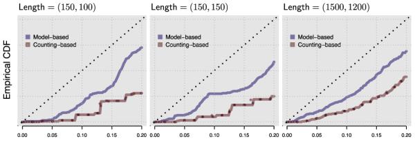
Partial empirical CDF of 1,000 p–values computed using different parameter estimates for data simulated under the null hypothesis. Three panels show different sequence lengths.

Finally, to assess the model fit of P(N_xy = n_xy)when motif prevalence is different between x and y, we simulated 100,000 sequence pairs in the following way. Sequence x was simulated from a phyloHMM with ζ_x →0 and sequence y from a model with ζ_y = 0.02. Taking single sequences from two different phyloHMMs corresponds to τ →∞.Figure 3 is analogous to Figure 1 and shows the result. We find that even when motif prevalence is different, our estimators of P(N_xy = n_xy) accurately capture the properties of the true, simulated distribution of N_xy.

Figure 3.

P(N_xy = n_xy) for TF motif differences for sequences with different motif prevalence (ζ_x vs. ζ_y).

5. MOTIF DIVERGENCE IN GENE REGULATORY ENHANCERS DURING CARDIAC DEVELOPMENT

To illustrate the use of motifDiverge on genome sequence data, we analyze a collection of gene regulatory elements identified via ChIP-seq for the active enhancer-marking histone modification histone 2 lysine 27 acetylation (H3K27ac) by Wamstad et al. [9]. This study identified genomic sequences marked by H3K27ac in mouse embryonic stem cells (ESCs) and at several subsequent developmental time points along the differentiation of ESCs into cardiomyocytes (CMs), which are beating heart cells. Our analysis uses these cell type specific enhancer sequences to illustrate applications of motifDiverge to both non-homologous and homologous sequences. We also leverage RNA-seq gene expression measurements from the same ESC and CM samples [9] to identify expressed TFs. Tissue development is a useful system for illustrating our approach, because active regulatory elements and TFs that are important for regulating gene expression differ across cell types and between species.

5.1 Motif divergence between mouse and human enhancer sequences

We first explored the use of motifDiverge to quantify motif differences between homologous sequences. For each of the 8,376 H3K27ac-marked enhancers from mouse CMs, we identified the homologous human sequence (if any) using the whole-genome, 30-way vertebrate multiple sequence alignments available from the UCSC Genome Browser (http://genome.ucsc.edu), which are based on the hg18 and mm9 genome assemblies. It is interesting to compare CM gene regulation between these two species, because there are a number of structural and electrophysiological differences between their hearts. We identified 1,617 orthologous human-mouse sequence pairs that were at least 20 nucleotides long. For each enhancer pair, we estimated the number of motif hits in the human and mouse sequence with JASPAR PSPMs (http://jaspar.genereg.net) for all 53 TFs expressed in mouse CMs (defined as those that have at least 10 sequence fragments per kilobase of sequence in the gene per million fragments aligned to the genome: RPKM >10). We set the log odds score threshold to achieve a Type I error rate of 5%. Our findings were fairly robust to this thresh-old choice (Appendix; Figure 4). Then we tested for TFs with significant differences in motif counts between human and mouse in each CM enhancer region using count-based parameter estimation. Model-based estimation produced p– values that were highly correlated with those from the count-based analysis (Appendix; Figure 5).

Figure 4.

Scatter plots of motifDiverge −log(p–values) comparing human versus mouse cardiomyocyte enhancers for all expressed TFs at different motif hit thresholds (0.01, 0.05, 0.1, 0.2).

Figure 5.

Correlation between motifDiverge p–values from count-based versus evolutionary model-based parameter estimation. Tests are for enrichment in mouse compared to human cardiomyocyte enhancers.

After adjusting for multiple testing using the Benjamini-Hochberg false discovery rate (FDR) controlling procedure [23], we found that a large percentage of enhancers (82%) show evidence of significant differences in motif counts for at least one TF (FDR < 5%; count-based parameter estimation). About two thirds of CM enhancers (66%) have significant differences in motif counts for multiple TFs, and several have significant differences for ten or more TFs. Conversely, most TFs only have significant differences in counts between human and mouse for a small percentage of CM enhancers. This suggests that differences in the motif composition of ESC and CM enhancers is driven mostly by a few TFs. The TFs with the largest percentage of enhancers showing significant differences are listed in Table (1). These TFs are promising candidates for understanding differences in CM gene regulation between humans and mice. Interestingly, Mycn, Jdp2 and Fhl1 have some enhancers with significantly more motifs in human and some enhancers with more motifs in mouse, suggesting that these TFs may target somewhat different sets of enhancers—and potentially different genes—in the two species.

Table 1.

Transcription factors with the most enhancers showing significant divergence in motif counts between human and mouse sequences, excluding those with more than 2% of enhancers showing discordant results between model-based and count-based parameter estimation methods

Transcription factors with more motifs in mouse
TF	Proportion of CM enhancers with more motifs in mouse
Egr1	0.137
Mycn	0.064
Fhl1	0.033
Pbx1	0.032
Jdp2	0.012
Transcription factors with more motifs in human
TF	Proportion of CM enhancers with more motifs in human
Mafk	0.275
Mycn	0.035
Creb3l2	0.033
Trp53	0.025
Jdp2	0.023
Srebf1	0.020
Fhl1	0.019
Gabpa	0.012
Deaf1	0.0093

5.2 Differences in motifs between enhancers active in different cell types

Next, we used motifDiverge to compare motif counts between non-homologous sequence pairs. This application also illustrates how motifDiverge can be applied to perform a single test to compare two sets of sequences. We concatenated the sequences of the 10,580 H3K27ac-marked regions in CMs to create a single, long sequence containing all the active enhancers for this cell type. Then, we generated a similar concatenation of all 7,159 enhancers from ESCs. Any genome sequence marked by H3K27ac in both ESCs and CMs was removed from both data sets, so that the resulting two ESC and CM enhancer sequences were non-overlapping. We predicted motifs in the ESC and CM sequences as described above with PSPMs for all 73 TFs expressed in either cell type. Then we tested for TFs with significant differences in motif counts between the combined enhancer regions of the two cell types. At FDR < 5%, we found 40 TFs with significantly more motifs in ESC enhancers and 27 TFs with significantly more motifs in CM enhancers.

To better understand the biological meaning of these results, we used the Wamstad et al. RNA-seq data to quantify the expression of each TF in ESCs and CMs. Several TFs are only highly expressed in one cell type, while others are expressed in both ESCs and CMs. The TFs with the most significant motif divergence included many that were highly expressed in the cell type with more motifs, but also some with low–though potentially biologically significant– expression levels (Table 2). This is not surprising, since TFs can function at low expression levels. Expression levels of some TFs were much higher in the cell type with more motifs compared to the other cell type (e.g., Gbx2 and Sox15 in ESCs, Egr1 in CMs), but in many cases expression was similar or even higher in the cell type with fewer motifs (e.g., Nkx2-5). This suggests that RNA-seq data might also be useful for filtering out significant motif differences that are not biologically meaningful; Nkx2-5 is not expressed in ESCs, making it unlikely that the additional motifs affect ESC gene regulation. More likely, these motifs reflect similarity in the Nkx2-5 motif to other TF’s motifs or usage of the ESC regulatory regions in other cell types where Nkx2-5 is expressed, a hypothesis that could be tested as RNA-seq data from more cell types becomes available. Finally, Nkx2-5 and many other TFs have multiple different motif models (PSPMs) in different databases, and results should also be compared across PSPMs for the same TF, which can be quite different from one another. In the case of Nkx2-5, enrichment in ESCs is not recapitulated with some of the alternative PSPMs, further supporting the idea that the ESC motif hits are not biologically meaningful. These analyses show how motifDiverge can be used to analyze data from ChIP-seq experiments and how RNA-seq data can be used to filter and interpret motifDiverge findings, leading to robust conclusions about the role of sequence differences in gene regulation.

Table 2.

Transcription factors with the most significant differences in TF motif counts between ESCs and CMs. Expression values are reads per kilobase per million fragments sequenced (RPKM)

Transcription factors with more motifs in ESC
TF	FDR adjusted p–value	ESC Expression	CM Expression
Rhox6	<1e-300	11.890	0.129
Pou3f1	<1e-300	15.081	0.380
Zfp187	<1e-300	8.215	13.816
Sox2	<1e-300	212.888	0.120
Hmbox1	<1e-300	4.799	12.281
Pou2f1	<1e-300	12.103	7.669
Sox12	<1e-300	22.933	23.458
Foxd3	<1e-300	20.746	0.038
Zfp105	<1e-300	10.949	4.216
Srf	<1e-300	33.402	42.569
Sox13	<1e-300	14.345	2.693
Tbp	<1e-300	15.609	5.676
Hbp1	<1e-300	17.552	28.762
Arid3a	<1e-300	5.055	15.516
Sox4	<1e-300	17.788	41.915
Pbx1	<1e-300	6.593	43.487
Gata6	<1e-300	0.152	75.887
Mafk	<1e-300	3.695	18.851
Pou5f1	<1e-300	669.960	0.043
Yap1	9.5e-294	51.1	57.6
Cebpb	5.3e-271	6.2	16.7
Gbx2	7.7e-258	22.7	0.01
Zfp652	5.1e-156	8.0	11.9
Dbp	4.1e-132	3.5	28.5
Elf3	1.1e-130	24.3	0.6
Zbtb12	3.2e-84	23.5	25.8
Tcf7	2.3e-75	16.3	7.6
Fhl1	4.7e-63	26.6	29.7
Nkx2-5	3.0e-60	0.9	177.6
Sox15	1.0e-42	14.1	0.1
Transcription factors with more motifs in CM
TF	FDR adjusted p–value	ESC Expression	CM Expression
Tcfap2c	<1e-300	23.884	0.055
Zic2	5.5e-248	26.8	0.1
Srebf1	1.1e-185	15.5	27.5
Esrrb	7.4e-98	85.2	2.4
Zic3	4.3e-92	38.6	0.07
Creb3l2	2.0e-69	1.3	50.1
Stat3	1.1e-62	8.4	21.8
Tgif1	5.6e-61	43.3	6.4
Smad3	1.8e-56	5.3	21.1
Myc	2.9e-53	32.0	4.2
Glis2	1.6e-49	12.5	12.9
Mlx	2.8e-35	18.3	7.03
Tcf3	1.2e-24	54.7	21.0
Mycn	2.6e-20	125.5	10.8
Xbp1	2.0e-18	18.8	20.5
Egr1	2.5e-18	19.9	192.2
Atf1	1.4e-17	26.3	7.2
Zbtb7b	2.7e-17	3.4	10.8

6. CONCLUSION

In this paper, we propose a new model for the difference in counts between two correlated Bernoulli trials representing numbers of TF motifs in a pair of DNA sequences. Our major results are the model derivation, accurate methods for parameter estimation, and a software package called motifDiverge that can be used to predict TF motifs and to perform tests comparing motif counts in two sequences. We illustrate the use of motifDiverge to discover TFs with significant differences in motifs (i) between two species, or (ii) between two cell types. These applications demonstrate the power of our methodology for discovering specific genes and regulatory mechanisms involved in species divergence and tissue development through careful analysis of ChIP-seq data.

Sequence divergence is usually measured in numbers of DNA substitutions or model-based estimates of rates of substitutions. These measures do not account for whether or not substitutions create or destroy TF motifs and are not well suited to quantify functional divergence [12]. Our tests capture how changes to DNA sequences affect their TF motif composition, and therefore they provide a more meaningful measure of divergence for regulatory regions. Hence, our model will be useful for understanding when non-coding mutations affect or do not affect the function of regulatory sequences. This information will enable, for example, identification of causal mutations in genomic regions identified as associated with diseases or other phenotypes. Since the majority of these genome-wide association study (GWAS) hits are outside of protein-coding regions [24], motifDiverge has the potential to have a large impact on human genetics research.

In future work, it would be interesting to extend our approach to model the joint distribution of multiple correlated Bernoulli trails and univariate summary statistics (e.g., sums, differences) of this distribution. As with two sequences, the main challenge is modeling correlations between the sequences. The phylogenetic tree models we used here can measure relationships between multiple homologous, but not equally related, DNA sequences; therefore they could provide a natural solution to this problem. Another interesting application would be to leverage motif divergence for phylogenetic tree construction, in place of the usual metric of overall sequence divergence. This could potentially be achieved in a maximum likelihood framework after development of a tree-based version of motifDiverge for multiple species.

We focus on comparing counts of TF motifs in two (possibly homologous) sequences, but our model is not specific to motifs in any way. The random variables N_x and N_y could represent other features of interest in two related DNA sequences, such as counts of microRNA binding sites, repetitive elements, polymorphisms, or experimentally measured events (e.g., ChIP-seq peaks). In fact, the two Bernoulli trials do not need to measure events on sequences, and our model could be applied to many other types of correlated count data.

APPENDIX

Derivation of Equation (3)

P(N_xy = n_xy) is a hypergeometric function for k_x = k_y

The probability mass function of N_xy for equal length sequences (Equation (2)) can be written as a sum: P(N_xy = n_xy) = Σ_jS_j, with the summands S_j given by Equation (1). Taking the ratio of two successive summands we get:

$$\begin{array}{cc}\hfill & S_{j+1}∕S_j=\hfill \\ \hfill & \frac{(n-n_{xy}-2j)(n-n_{xy}-2j-1)}{(j+n_{xy}+1)(j+1)}\frac{p_{10}{p}_{01}}{{(1-p_{10}-p_{01})}^2}=\hfill \\ \hfill & \frac{(j+\frac{n_{xy}-n}{2})(j+\frac{n_{xy}+1-n}{2})}{(j+n_{xy}+1)(j+1)}\frac{4p_{10}{p}_{01}}{{(1-p_{10}-p_{01})}^2}.\hfill \end{array}$$ (12)

We note that this is a rational function in j, n_xy and n and identifies the arguments (n_xy − n)/2, (n_xy − n + 1)/2 and (n_xy + 1) of the Gaussian hypergeometric function in Equation (3)[19].

Derivation of Equation (8)

Error bound for evaluating P(N_xy = n_xy) for k_x = k_y

Let w_j := S_j+1/S_j. From Equation (12), we get that increasing j decreases the numerator S_j+1 and increases the denominator S_j, so that w_j is decreasing in j. Therefore, there exists j₋,with w_j− < 1 (i.e., the summands S_j are decreasing for j ≥ i₋). The error ε(j₊) of truncating the sum over j at j₊ ≥ j₋ is then:

$$\begin{array}{cc}\hfill & ∊\left(j_{+}\right)=\hfill \\ \hfill & \sum _{j=j_{+}+1}^{\lfloor \frac{n-n_{xy}}{2}\rfloor }{S}_j=\stackrel{\lfloor \frac{n-n_{xy}}{2}\rfloor }{\sum _{j=j_{+}+1}^2}{w}_{j-1}{w}_{j-2}\dots {w_j}_{+}{S}_{j_{+}}<\hfill \\ \hfill & \sum _{j=1}^{\lfloor \frac{n-n_{xy}}{2}\rfloor -j_{+}}{w}_{j_{+}}^j{S}_{j_{+}}=S_{j_{+}}\left(\frac{1-w_{j_{+}}^{\lfloor \frac{n-n_{xy}}{2}\rfloor -j_{+}}}{1-w_{j_{+}}}-1\right),\hfill \end{array}$$ (13)

where we have used the following: (i) S_j =(S_j /S_j−1)S_j−1 = wj−1S_j−1,(ii) S_j are decreasing for j ≥ j₋,(iii) S_j ≤ 1are non-negative multinomial probabilities (see Equation (2)), and (iv) the geometric sum. Thus, to estimate the probability mass function of N_xy to a desired precision ε, S_j an be truncated at the first j₊ ≥ j₋ for which E(j₊) ≤ ε.

Derivation of Equation (9)

Recurrence relation for P(N_xy = n_xy) for k_x = k_y

Let P(N_xy = n_xy) = Σ_jS(j,n_xy, n), where the summands S(j,n_xy, n) are taken from Equation (2). Recurrence relations in n and n_xy can be obtained via the Zeilberger algorithm [19], for instance as implemented in the computer algebra system Maxima (http://sourceforge.net/projects/maxima). For a recurrence in n_xy, the Maxima code is:

(%1) Sj : n!/((n_{xy}+j)!*i!*(n-n_{xy}-2*j)!)

   *p10^(n_{xy}+j)*p01^j*(1-p10-p01)^(n-n_{xy}-2*j) $

(%2) load(zeilberger) $

(%3) Zeilberger(Sj,j,n_{xy});

(%o3) [[-(j*(n+n_{xy}+2)*p10)/(n_{xy}+j+1),

   [(n-n_{xy})*p10,(n_{xy}+1)*(p10+p01-1),

   -(n+n_{xy}+2)*p01]]]

This output defines the following quantities:

$$\begin{array}{cc}\hfill & a_0(n_{xy},n)=(n-n_{xy})p_{10}\hfill \\ \hfill & a_1(n_{xy},n)=-(n_{xy}+1)(1-p_{10}-p_{01})\hfill \\ \hfill & a_2(n_{xy},n)=-(n+n_{xy}+2)p_{10}\hfill \\ \hfill & R(j,k,n_{xy})=-\frac{j(n+n_{xy}+2)p_{10}}{n_{xy}+j+1},\hfill \end{array}$$

which satisfy the recurrence relation

$$\begin{array}{cc}\hfill & a_0(n_{xy},n)S(j,n_{xy},n)+a_1(n_{xy},n)S(j,n_{xy}+1,n)+\hfill \\ \hfill & a_2(n_{xy},n)S(j,n_{xy}+2,n)=\hfill \\ \hfill & R(j+1,n_{xy},n)S(j+1,n_{xy},n)-R(j,n_{xy},n)S(j,n_{xy},n).\hfill \end{array}$$ (14)

Summing Equation (14) over j gives the recurrence for P(N_xy = n_xy). We confirm that the right hand side is zero:

$$\begin{array}{cc}\hfill & a_0(n_{xy},n)P(N_{xy}=n_{xy})+a_1(n_{xy},n)P(N_{xy}=n_{xy}+1)+\hfill \\ \hfill & a_2(n_{xy},n)P(N_{xy}=n_{xy}+2)=\hfill \\ \hfill & \sum _{j=0}^{\lfloor \frac{n-n_{xy}}{2}\rfloor }(R(j+1,n_{xy},n)S(j+1,n_{xy},n)-R(j,n_{xy},n)S(j,n_{xy},n))=\hfill \\ \hfill & R\left(\lfloor \frac{n-n_{xy}}{2}\rfloor +1,n_{xy},n\right)S\left(\lfloor \frac{n-n_{xy}}{2}\rfloor +1,n_{xy},n\right)-\hfill \\ \hfill & R(0,n_{xy},n)S(0,n_{xy},n)=0.\hfill \end{array}$$

That R(0,n_xy, n) = 0 follows straight from the definition, and that $S(\lfloor \frac{n-n_{xy}}{2}\rfloor +1,n_{xy},n)$ = 0 follows via S_j+1 = (S_j+1/S_j )S_j and Equation (12).

Derivation of Equation (10)

In-sequence and between-sequence correlation

As mentioned in the main text, PSPM based annotation of motifs generates in-sequence dependence that is not per-se accounted for in our model. Suppose there is a first order (Markov) dependence of X_i on X_i−1, quantified by the parameter λ_x (and likewise for Y_i). Under these assumptions the expected value for N_x is still k_xp, but for the variance we find [20]:

$$\begin{array}{cc}\hfill & \mathrm{Var}\left(N_x\right)=\hfill \\ \hfill & k_{x}p(1-p)+\frac{2p(1-p)({\lambda }_x-p)}{1-{\lambda }_x}\times \hfill \\ \hfill & \left[(k_x-1)-\frac{{\lambda }_x-p}{1-{\lambda }_x}\left(1-{\left[\frac{{\lambda }_x-p}{1-p}\right]}^{k_x}\right)\right],\hfill \end{array}$$ (15)

and an equivalent expression for N_y. For N_xy = N_x −Ny we then find (assuming no between-sequence dependence)

$$\mathrm{Var}\left(N_{xy}\right)=k_{x}p(1-p)+A(p,{\lambda }_x,k_x)+k_{y}q(1-q)+A(q,{\lambda }_y,k_y)$$ (16)

where A(·,·,·) represents the second term in the variance formula in Equation (15) and Cov(X_i,Y_i) = 0. Comparing Equation (16) with Equation (7), substituting p = p₁₁ + p₁₀ and q = p₁₁ + p₀₁ we arrive at Equation (10) after some algebra. Note that a negative correlation between X_i and X_i+1 decreases the variance in N_x = X_i, and similarly i for N_y. If both sequences have negative correlation between subsequent successes, the variance of N_xy decreases. This is the same effect a correlation between X_i and Y_i has on the variance of N_xy.

Parameter estimates contributing to $\widehat{\rho }$ in Equations (10) and (11)

Count-based and model-based parameter estimates

Here we describe estimates for the parameters λ_x = λy =: λ (for independent sequences)and p1→1 (for homologous sequences with alignment). These quantities reflectin-sequence and between-sequence dependencies, respectively: λ = P(X_i = 1|X_i−1 = 1) and p1→1 = P(Y_i = 1|X_i = 1), see Section 2.2.5 in the main text. We assume that the in-sequence dependence is the same in x and y, that motif gains and losses are time-reversible (i.e., P(Y_i = 1|X_i = 1) = P(X_i = 1|Y_i = 1) and present count-based estimates as well as estimates based on a phylogenetic hidden Markov model (phyloHMM).

Count-based estimates

For a count-based estimate for λ, we count the number of adjacent motif hits in both x and y, and then divide it by the number of overall motif hits in both sequences. This is analogous to the estimate p̂ for the success probability of the two B_inomial trials X and Y, as described in the main text. For p̂_1→1, in turn, we count the number of congruent motif hits in x and y from alignments, and then divide the result by the overall number of motif hits in x. The advantage of both these estimates is that they do not take much effort to calculate. The downside is that typically p is small (for instance because a strict Type I error cutoff t in motif prediction, see Section 2.1). This, in turn, means that (especially for short and intermediate length sequences) not many adjacent or congruent motif hits will be observed. Therefore these count-based estimates can be very variable in those situations.

Model-based estimates

To overcome the variability in the count-based estimates described above to some extent, we assume a phyloHMM as an underlying, generative model for the two sequences x and y. For this approach we require a sequence alignment of x and y. Essentially, we fit the phyloHMM to our observation (the sequences x and y, plus the corresponding motif hits) and then derive the parameters of interest as large sample properties from the fitted model. As described in Section 4.1, the phyloHMM consists of three states: a background state (corresponding to a neutral evolutionary model), a motif state, and a state for the reverse complement of the motif. First, we model the transition probabilities to be ζ/2 for background-to-motif and motif-to-motif transitions, and 1 −ζ for background-to-background and motif-to-background transitions. We then fix the ζ in such a way that

$$E_O\left[P_{S~O}(T\left(S\right)>t)\right]=\widehat{p},$$ (17)

where p̂ is our count-basedestimate of the success probability, S is a nucleotide sequence of motif-length (with log odds score T(S)) emitted by the phyloHMM Ψ as either of the two sequences, and O is the state-path of motif-length generated by the Markov chain in Ψ that underlies the emission of S. Note that the left-hand sidein Equation (17) depends on ζ because the probability for each state-path depends on the transition probabilities; but the LHS is independent of τ (the evolutionary time between sequences x and y),because the Ψ is time-reversible and S is a “marginalized” single sequence, not a sequence-pair. To evaluate the expectation in Equation (17) we enumerate all possible state-paths O and calculate (i) their Type I motif-hit error according to the PSPM and background distribution used for motif annotation (see Section 2.2), and (ii) their probability of occurrence from the equilibrium frequencies of the Markov chain. This yields an estimate $\widehat{\zeta }$.

Next, to obtain an estimate for τ we maximize the likelihood of the sequences x and y:

$$\widehat{\tau }={\mathrm{argmax}}_{\tau }L((x,y)\mid \Psi (\tau ,\widehat{\zeta })),$$

where L() denotes the likelihood of jointly observing x and y. Overall this procedure yields a fully specified (fitted) phyloHMM $\Psi (\widehat{\tau },\widehat{\zeta })$.

Finally, we use this fitted phyloHMM to obtain estimates for λ and p_1→1. To that end we generate two very long (100,000 nucleotides or longer) sequences and take (i) $\widehat{\lambda }$ be the fraction of adjacent motif hits, and (ii)p̂_1→1 to be the fraction of motif hits that is congruent between the two generated sequences. We note that it is straightforward to obtain bounds for these estimates via B_inomial tail inversion [25].

Note that highly similar, well-aligned sequences will lead to short estimated evolutionary times $\widehat{\tau }$, and therefore high values for p̂_1→1, which will in-turn lead to large estimates of $\widehat{\rho }$ in Equation (11). Conserved motif instances in both sequences will, during the estimation procedure, “vote” for larger estimates of ζ and for smaller estimates of τ;non-conserved motif hits, on the other hand, will still favor large ζ, but also large τ (in contrast to small τ). Long evolutionary times are the only way the null-model (of no difference in motif-prevalence between the two sequences) can account the creation/destruction of motif hits. The evolutionary model also accounts for the fact that some nucleotide changes are more likely than others, and that some motifs are therefore more likely to be lost and gained than others, based on their nucleotide composition. Finally, more realistic evolutionary models that explicitly include insertions and deletions could in principle be utilized in this framework.

Effects of the threshold used to identify motif hits

We investigated the sensitivity of motifDiverge findings to the choice of threshold used to identify motif hits in each sequence. Specifically, for the analysis of human versus mouse CM enhancers (Section 5.1), we tested the robustness of our results by varying the log odds score threshold across a range of values: 1%, 5%, 10%, 20%. We found that the resulting motifDiverge p–values are correlated (Figure 4) across thresholds, with higher correlation at more similar thresholds, as expected. We also observed that our conclusions about human versus mouse enhancer motif content are not dramatically affected by the choice of threshold.

Effects of parameter estimation methods

We compared several methods of motifDiverge model parameter estimation in our analysis of human versus mouse CM enhancers (Section 5.1). Overall, model-based estimation identified more TFs with significantly different numbers of motifs between the two species. We found that 100% of enhancers had at least one TF with significant differences compared to 82% with count-based estimation. However, motifDiverge p–values from the two approaches are highly correlated (Figure 5). For many TFs, including Smad3, Atf6, Fhl1, Jdp2, and Arnt, there were almost no differences in the number of enhancers with significant losses or gains when comparing count-based and model-based estimation (<1% of enhancers discordant). On average across TFs, about 2% of enhancers produced discordant results when using a Type I error threshold of 5% for calling motif hits and FDR < 0.05 for motifDiverge tests. No TFs had more than 5% discordant results across enhancers. When using a stricter Type I error threshold of 1% for calling motif hits, results were more discordant between count-based and model-based estimation procedures (typically 10%−30% discordant). Thus, while our simulations indicate that model-based estimation can be more sensitive, we found in practice that for species at the divergence of human and mouse, accounting for the phylogenetic relationship between sequences does not have a big impact on motifDiverge results. Both options are available in the R package and can be explored by users for their particular application.

REFERENCES

- [1].Rivera CM, Ren B. Mapping human epigenomes. Cell. 2013 Sep;155:39–55. doi: 10.1016/j.cell.2013.09.011. [DOI] [PMC free article] [PubMed] [Google Scholar]
- [2].McGettigan PA. Transcriptomics in the RNA-seq era. Current Opinion in Chemical Biology. 2013 Feb;17:4–11. doi: 10.1016/j.cbpa.2012.12.008. [DOI] [PubMed] [Google Scholar]
- [3].Ozsolak F, Milos PM. RNA sequencing: advances, challenges and opportunities. Nat Rev Genet. 2011;12(2):87–98. doi: 10.1038/nrg2934. [DOI] [PMC free article] [PubMed] [Google Scholar]
- [4].John S, Sabo PJ, Canfield TK, Lee K, Vong S, Weaver M, Wang H, Vierstra J, Reynolds AP, Thurman RE, Stamatoyannopoulos JA. Genome-scale mapping of DNase I hypersensitivity. Current protocols in molecular biology/edited by Frederick M. Ausubel … [et al.] 2013 Jul;Chapter 27:21.27–21.27.20. doi: 10.1002/0471142727.mb2127s103. Unit. [DOI] [PMC free article] [PubMed] [Google Scholar]
- [5].Giresi PG, Kim J, McDaniell RM, Iyer VR, Lieb JD. FAIRE (Formaldehyde-Assisted Isolation of Regulatory Elements) isolates active regulatory elements from human chromatin. Genome Research. 2007 Jun;17:877–885. doi: 10.1101/gr.5533506. [DOI] [PMC free article] [PubMed] [Google Scholar]
- [6].Furey TS. ChIP-seq and beyond: new and improved methodologies to detect and characterize protein-DNA interactions. Nat Rev Genet. 2012 Dec;13:840–852. doi: 10.1038/nrg3306. [DOI] [PMC free article] [PubMed] [Google Scholar]
- [7].Wang C, Zhang MQ, Zhang Z. omputational identification of active enhancers in model organisms. Genomics, Proteomics and Bioinformatics. 2013 Jun;11:142–150. doi: 10.1016/j.gpb.2013.04.002. [DOI] [PMC free article] [PubMed] [Google Scholar]
- [8].de Laat W, Duboule D. Topology of mammalian developmental enhancers and their regulatory landscapes. Nature. 2013 Oct;502:499–506. doi: 10.1038/nature12753. [DOI] [PubMed] [Google Scholar]
- [9].Wamstad JA, Alexander JM, Truty RM, Shrikumar A, Li F, Eilertson KE, Ding H, Wylie JN, Pico AR, Capra JA, Erwin G, Kattman SJ, Keller GM, Srivastava D, Levine SS, Pollard KS, Holloway AK, Boyer LA, Bruneau BG. Dynamic and Coordinated Epigenetic Regulation of Developmental Transitions in the Cardiac Lineage. Cell. 2012;151(1):206–220. doi: 10.1016/j.cell.2012.07.035. [DOI] [PMC free article] [PubMed] [Google Scholar]
- [10].Maston GA, Landt SG, Snyder M, Green MR. Characterization of enhancer function from genome-wide analyses. Annual Review of Genomics and Human Genetics. 2012;13(1):29–57. doi: 10.1146/annurev-genom-090711-163723. [DOI] [PubMed] [Google Scholar]
- [11].Stormo GD. DNA binding sites: representation and discovery. Bioinformatics. 2000 Jan;16:16–23. doi: 10.1093/bioinformatics/16.1.16. [DOI] [PubMed] [Google Scholar]
- [12].Ritter DI, Li Q, Kostka D, Pollard KS, Guo S, Chuang JH. The Importance of Being Cis: Evolution of Orthologous Fish and Mammalian Enhancer Activity. Molecular Biology and Evolution. 2010;27(10):2322–2332. doi: 10.1093/molbev/msq128. [DOI] [PMC free article] [PubMed] [Google Scholar]
- [13].Rahmann S, Muller T, Vingron M. On thepower of profiles for transcription factor binding site detection. Statistical Applications in Genetics and Molecular Biology. 2003;2 doi: 10.2202/1544-6115.1032. Article7. MR2086500. [DOI] [PubMed] [Google Scholar]
- [14].Siddharthan R. Dinucleotide weight matrices for predicting transcription factor binding sites: generalizing the position weight matrix. PLoS ONE. 2010;5(3):e9722. doi: 10.1371/journal.pone.0009722. [DOI] [PMC free article] [PubMed] [Google Scholar]
- [15].Zhao Y, Ruan S, Pandey M, Stormo GD. Improved models for transcription factor binding site identification using nonindependent interactions. Genetics. 2012 Jul;191:781–790. doi: 10.1534/genetics.112.138685. [DOI] [PMC free article] [PubMed] [Google Scholar]
- [16].Mathelier A, Wasserman WW. The next generation of transcription factor binding site prediction. PLoS Comput Biol. 2013;9(9):e1003214. doi: 10.1371/journal.pcbi.1003214. [DOI] [PMC free article] [PubMed] [Google Scholar]
- [17].Weirauch MT, Cote A, Norel R, Annala M, Zhao Y, Riley TR, Saez-Rodriguez J, Cokelaer T, Vedenko A, Talukder S, Agius P, Arvey A, Bucher P, Callan CG, Chang CW, Chen C-Y, Chen Y-S, Chu Y-W, Grau J, Grosse I, Jagannathan V, Keilwagen J, Kiee̷basa SM, Kinney JB, Klein H, Kursa MB, Lahdesmaki H, Laurila K, Lei C, Leslie C, Linhart C, Murugan A, Myvsivckova A, Noble WS, Nykter M, Orenstein Y, Posch S, Ruan J, Rudnicki WR, Schmid CD, Shamir R, Sung W-K, Vingron M, Zhang Z, Bussemaker HJ, Morris QD, Bulyk ML, Stolovitzky G, Hughes TR. Evaluation of methods for modeling transcription factor sequence specificity. Nature Biotechnology. 2013;31(2):126–134. doi: 10.1038/nbt.2486. [DOI] [PMC free article] [PubMed] [Google Scholar]
- [18].Pape UJ, Rahmann S, Sun F, Vingron M. Compound poisson approximation of the number of occurrences of a position frequency matrix (PFM) on both strands. Journal of computational biology: a journal of computational molecular cell biology. 2008 Jul;15:547–564. doi: 10.1089/cmb.2007.0084. MR2425441. [DOI] [PMC free article] [PubMed] [Google Scholar]
- [19].Petkovsek M, Wilf HS, Zeilberger D. AK Peters, Ltd.; 1996. A = B. MR1379802. [Google Scholar]
- [20].Klotz J. Statistical Inference in Bernoulli Trials with Dependence. The Annals of Statistics. 1973 Mar;1:373–379. MR0381103. [Google Scholar]
- [21].Hubisz MJ, Pollard KS, Siepel A. PHAST and RPHAST: phylogenetic analysis with space/time models. Briefings in Bioinformatics. 2011;12(1):41–51. doi: 10.1093/bib/bbq072. [DOI] [PMC free article] [PubMed] [Google Scholar]
- [22].Tukey John W. Statistical papers in honor of George W. Snedecor. The Iowa State University Press; 1972. Some Graphic and Semigraphic Displays; pp. 293–316. MR0448637. [Google Scholar]
- [23].Benjamini Y, Hochbert Y. Controlling the False Discovery Rate: A practical and powerful apporach to multiple testing. Journal of the Royal Society B. 1995;57(1):289–300. MR1325392. [Google Scholar]
- [24].Hindorff LA, Sethupathy P, Junkins HA, Ramos EM, Mehta JP, Collins FS, Manolio TA. Potential etiologic and functional implications of genome-wide association loci for human diseases and traits. Proceedings of the National Academy of Sciences of the United States of America. 2009;106:9362–9367. doi: 10.1073/pnas.0903103106. [DOI] [PMC free article] [PubMed] [Google Scholar]
- [25].Kaariainen M, Langford J. Proceedings of the 22Nd International Conference on Machine Learning. New York, NY, USA: 2005. A Comparison of Tight Generalization Error Bounds; pp. 409–416. ACM. [Google Scholar]