

Abstract
DNA profiling of biological material from scenes of crimes is often complicated because the amount of DNA is limited and the quality of the DNA may be compromised. Furthermore, the sensitivity of STR typing kits has been continuously improved to detect low level DNA traces. This may lead to (1) partial DNA profiles and (2) detection of additional alleles. There are two key phenomena to consider: allelic or locus ‘drop-out’, i.e. ‘missing’ alleles at one or more genetic loci, while ‘drop-in’ may explain alleles in the DNA profile that are additional to the assumed main contributor(s). The drop-in phenomenon is restricted to 1 or 2 alleles per profile. If multiple alleles are observed at more than two loci then these are considered as alleles from an extra contributor and analysis can proceed as a mixture of two or more contributors. Here, we give recommendations on how to estimate probabilities considering drop-out, Pr(D), and drop-in, Pr(C). For reasons of clarity, we have deliberately restricted the current recommendations considering drop-out and/or drop-in at only one locus. Furthermore, we offer recommendations on how to use Pr(D) and Pr(C) with the likelihood ratio principles that are generally recommended by the International Society of Forensic Genetics (ISFG) as measure of the weight of the evidence in forensic genetics. Examples of calculations are included. An Excel spreadsheet is provided so that scientists and laboratories may explore the models and input their own data.
Keywords: Forensic genetics, Recommendations on forensic STR typing, Probabilistic models in forensic genetics, Drop-in/drop-out, Likelihood ratio
1. Introduction
The present recommendations are intended to guide scientists and laboratories that wish to use probabilistic reasoning to interpret DNA profiles where drop-out and/or drop-in is considered. The methods used can be undertaken with the likelihood ratio (LR) principle that was previously recommended for crime case work by the DNA Commission of the International Society of Forensic Genetics (ISFG) [1] and for paternity/relationship testing by the Paternity Testing Commission of the ISFG [2,3].
A previous ISFG DNA commission evaluated the advantages of the likelihood ratio principle in relation to DNA mixture interpretation [1]. These recommendations are still valid, and the present work expands on the previous publication.
Many practitioners find the theory difficult to follow, and doubtless this inhibits the uptake of new statistical models. The purpose of the present recommendations is to explain established theory that is more than 10 years old [4]. Although the theory is easily extended to multiple loci and multiple contributors, in the present recommendations, we consider only one locus in the profile but allow for drop-in and drop-out at that locus [4]. Nevertheless, an appreciation of the basic principles that are enumerated in this paper will greatly facilitate understanding of more complex (multi-locus, multi-contributor) examples. Even so, the simplest models are still too complex for routine hand-calculation and the formulae themselves are not easily adapted to computer algorithms. This problem was solved by Curran et al. [5] who introduced set theory in order to enable the calculations to be made, and more importantly to enable expansion from the single to multiple contributors. This theory forms the basis of available software approaches, but we do not attempt to explain set theory in this paper.
The DNA Commission now considers it timely to establish recommendations on the application of these principles to more complex DNA results in light of the rapid development of open-source [6] and closed source [5,7] bio-statistical tools that are now the subject of court room evaluation in a number of countries.
With any DNA profile, if drop-out and/or drop-in are possible (this includes any partial DNA profile), it is not possible to think only in terms of a match or non-match, the various possibilities can only be properly evaluated in probabilistic terms by means of the likelihood ratio principles (see Section 8 for a discussion).
We provide two examples applied to a single locus of a sample from a single contributor. The first example shows how to interpret a partial profile where drop-out may have occurred, and the second example shows how to interpret a profile where simultaneous drop-out and drop-in events have occurred. This would usually result in exclusion using traditional methods of interpretation. The theory can be extended to complex mixtures, not described here. Neither do we detail sub-population correction (FST) but this extension is straightforward and described by Curran et al. [8].
In real life, crime-stains will show additional complexities across multiple loci. Mixtures will be common, with varying amounts of drop-out levels per contributor. The primary purpose of the paper is to demonstrate why, for many samples, classical binary models are largely inferior to the probabilistic approach described here – without going into the additional details and of how to incorporate mixture theory (e.g. Ref. [5]).
Clearly the adoption of probabilistic models has been inhibited by the complexity of concepts that are largely outside the experience of case-working forensic scientists, coupled with lack of suitable training opportunities. New initiatives, such as the EU-FP7 funded ‘Euroforgen’ network project http://www.eurofor-gen.eu/ seek to remedy this problem, strongly supported by the ISFG that is providing additional training courses.
Some laboratories will wish to quickly adopt probabilistic methods ahead of the main-stream forensic community. This ISFG DNA commission strongly supports this approach, since it will encourage others to follow. In this context, it should be noted that the approach described here still requires a rigid assessment of the overall quality of a given DNA profile and its suitability for further analysis based on criteria described in the laboratory’s quality management guidelines.
In conjunction with this paper, an Excel workbook (see electronic supplement) has been released on the ISFG website http://www.isfg.org/Software. The workbook enables scientists and laboratories to explore the methods described using their own data. Further material will be provided as it becomes available.
2. Interpretation of a heterozygous, unmixed sample using probabilistic reasoning
For a simple heterozygous genotype, the likelihood ratio is formulated from two alternative hypotheses. The numerator evaluates the strength of the evidence (E) if the prosecution hypothesis (Hp) is true and the denominator evaluates the strength of the evidence if the defence hypothesis (Hd) is true. The likelihood ratio is formulated by comparing the two hypotheses as follows:
In its simplest form, Hp usually specifies the condition that: ‘the DNA profile came from the suspect’ and Hd specifies the condition that: ‘the DNA profile came from an unknown unrelated individual’. Hypotheses may be much more complex than this. For example, multiple contributors may be considered in admixture, and relatedness may be an issue if a brother can be the originator of the DNA profile. However, in this paper, we restrict the discussion to a single locus where the alternative hypotheses are restricted to a single suspect (Hp) vs. one (unrelated) unknown contributor (Hd). The terms Hp, Hd and E are convenient mathematical notations (an alternative way is to think in terms of ‘what-if’’ scenarios; see Section 4).
The alleles are designated a and b (Fig. 1). For convenience only, we further assume that the peak heights of each allele are above a ‘stochastic threshold’ T [9],1 where this threshold is such that the probability of drop-out Pr(D) of an allele above T will be almost zero. The level may be determined relative to a pre-determined Pr(D) by using logistic modelling [9] (see Appendix B). In the example illustrated in Fig. 1, there is no drop-out to consider if the suspect (S) is ab and the crime stain (E) is also ab.
Fig. 1.
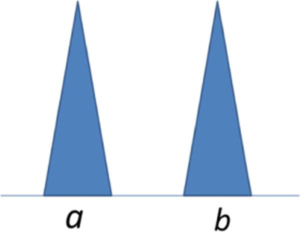
An example of a simple heterozygote profile where the suspect reference sample (S) and the crime stain (E) are identical.
3. The match probability and the likelihood ratio
The probability of match is the chance of a random match between a profile that is evidential (e.g. the crime-stain) and a profile that is from a specified individual such as the ‘suspect’ or the ‘random, unrelated’ contributor, whereas the likelihood ratio is a calculation of the ratio of probabilities of observing the DNA under two alternative hypotheses.
4. Likelihoods are conditional – they evaluate ‘what-if’ scenarios
We can think of likelihoods as evaluating ‘what-if’ scenarios. As an example: what-if the suspect really did contribute to the crime stain? If true, then the observation that the crime stain and the suspect have the same profile is to be expected and the probability of a match is 1, given Hp. This forms the numerator of the likelihood ratio equation.
Continuing the example, the alternative proposition is that someone other than the suspect must have deposited the crime stain. The denominator of the likelihood ratio equation deals with alternative explanations. This asks: what is the chance of observing the evidence if the suspect has not deposited the crime stain? Often this is calculated as the probability of observing the profile among unrelated, randomly selected individuals, i.e. the Hardy–Weinberg expectation, Pr = 2papb (where the allele frequencies are pa and pb, respectively).
Putting the numerator and denominator together, we form the ‘classical’ likelihood ratio:
The likelihood ratio provides a relative and numeric ‘strength of evidence’ of one hypothesis compared to its alternative. This assessment is always binary if the ‘classical’ approach is used. Either there is a match or non-match. This is why the numerator is always one if a match has been declared.2
If the LR is greater than one, it supports the hypothesis of inclusion, and if it is less than one, it supports the alternative hypothesis of exclusion.
5. Allele drop-out leads to a partial DNA profile that does not match the suspect’s reference profile
When the DNA quantity is sufficient to generate peaks above the (arbitrary) stochastic threshold, T, and the two alleles are a balanced heterozygote, a ‘match’ between the donor and the crime stain is usually seen (Fig. 1). As the template DNA level decreases, the signal level decreases and the heterozygote balance deteriorates. This occurs because of ‘stochastic’ or random effects that have previously been well characterised [10,11]. Allele drop-out is an extreme example of heterozygote imbalance, where one allele falls below the limit of detection threshold (LDT). Many laboratories have typically set this level to 50rfu – this value can vary both between laboratories and methods or processes used. The inevitable consequence of allele drop-out is that a partial profile is generated. This means that the crime-stain DNA profile may not match the DNA profile of the hypothesised contributor.
Allele drop-out is defined as a signal that falls below the LDT. Often, a signal that could represent an allele is present but it cannot be distinguished from irrelevant ‘noise’. The critical issue is that there is uncertainty about whether the allele is present or not.
6. The terms inclusion and exclusion are binary (absolute) determinants
Consequently, if there is any uncertainty in a pre-assessment, then it follows that there is uncertainty about the genotype, and this means that the probability of a proposed match must be less than one and greater than zero. This is often referred to as ‘inconclusive’ using the ‘classical’ approach.
Fig. 2 shows an example where allele b may have dropped out. There is uncertainty about the genotype of the crime stain. In this example the evaluated hypotheses are: Hp: the suspect contributed to the crime-sample, Hd: an unknown person, unrelated to the suspect contributed to the sample. The DNA profile could have come from the suspect if allele b dropped out. However, in the ‘classical’ approach, this yields a probability of zero under Hp, because the uncertainty in the crime stain genotype is not taken into account.
Fig. 2.
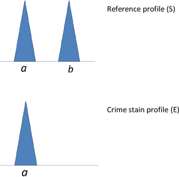
An example where the reference sample is type ab and the crime stain is type a.
If the DNA profile has not come from the suspect, the genotype could either be explained as a heterozygote, with allele a, and dropout of any other allele – including allele b if the true donor has the same genotype as the suspect. Alternatively, the true donor could be homozygote, where both alleles are type a, if no drop-out has happened.
A drop-out event in the crime-stain DNA profile evidence is often evaluated using the ‘2p’ rule [12]. For example, either: 2papF (under Hd), where pF = 1, or alternatively:
The virtual allele Q (frequency pQ =1−pa) is also used to signify that any allele may be present, except for allele a. Q is considered in the heterozygote part of the calculation (see Appendix A for a detailed explanation of the ‘virtual’ Q and F alleles).
7. How can uncertainty of matches be accommodated?
7.1. Drop-out
The drop-out probability Pr(D) depends upon the observed allele or the amount of DNA tested. The lower the peak height of a ‘surviving’ allele, the greater the probability that an unseen companion allele has dropped out. Pr(D) can be estimated by logistic analysis [13,14] or by using an empirical approach – for example [15]. With highly sensitive methods (34 cycles, and new generation analytical instruments such as the AB 3500 series) high allele peaks, for low template or degraded samples, may be associated with occasional drop-out. When such a profile is evaluated probabilistically, it will decrease the strength of evidence. Further details are provided in Appendix B to carry out the experiment in order to generate data for logistic analysis.
Fig. 3 shows the LR as a function of the Pr(D). The LRmix module in the open-source software package Forensim offers biostatistical tools to perform this analysis [6].
Fig. 3.
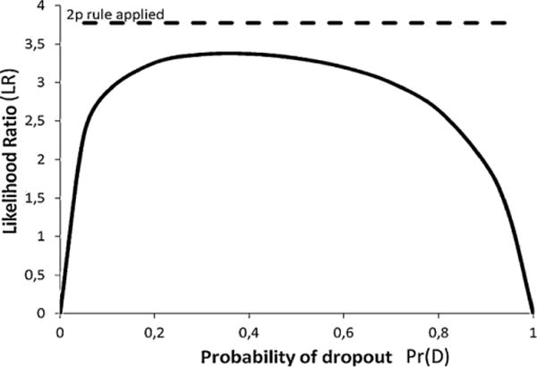
Effect of Pr(D) on LR. S is ab, E is a. The likelihood ratio LR = Pr(E\Hp)/Pr(E\Hd) is plotted as a function of Pr(D) ∈ [0,1]. Locus D18S51 frequencies are used as an example, where allele a corresponds to D18S51 allele 13 (frequency: 0.135). Using the 2p rule: LR = 1/(2pa) = 1/(2 × 0.135) = 3.8 (dashed line).
7.2. Drop-in and contamination
The drop-in phenomenon was originally described by Gill et al. [4]. Drop-in will often affect casework samples [16]. There is no absolute method to determine if drop-in or contamination has occurred in a casework sample, but negative controls can be used to estimate the probability of drop-in within casework samples. In this context, we distinguish between drop-in and contamination. The latter term specifically describes more than two or more alleles that come from a single individual. Conversely, drop-in alleles come from different individuals. The distinction is important, because the assumption of independence enables the use of the product rule to multiply drop-in probabilities, whereas this is not valid if the events are dependent. Drop-in and contamination may have occurred even if the negative control is ‘clean’ and does not show any allele at all.
To recap, the drop-in event is relatively rare and is measured by reference to negative controls. If n negative controls are analysed and there are x spurious alleles observed (where the counts are restricted to one or two events per profile) then Pr(C) is estimated as x/n. Its level will increase as the sensitivity of the process increases – e.g. by increasing the number of PCR cycles; introduction of new highly sensitive genetic analysers like the AB 3500 series; new multiplex kits; mixtures [17].3 To calculate the risk of a drop-in event in a casework profile, we multiply together the probability of drop-in with the probability of the specific allele a that is conditioned to have dropped in: Pr(C)pa [4].
7.3. Contamination is distinct from drop-in
Contamination profiles are indistinguishable from any other mixed profile and we define these specifically as profiles that are unrelated to the case. Evidential material may be ‘contaminated’ before the crime event with ‘background’ DNA profiles. Plastic-ware contamination is an example of contamination (in the laboratory). There is no information inherent in the DNA profile that provides information about ‘how’ or ‘when’ the profile was transferred. These issues are dealt with separately at trial where the ‘relevance’ of the evidence is decided by the court (the scientist may be asked to comment on issues of transfer and persistence to assist the court).
However, the calculation of the likelihood ratio addresses the alternative propositions that relate solely to the specific issue of ‘source’ of the DNA profile. The expert will evaluate two alternative hypotheses within the likelihood ratio calculation as described in Section 2:
What is the strength of the evidence if the DNA profile originated from the suspect?
What is the strength of the evidence if the DNA profile originated from an unknown unrelated individual?
8. The classical model vs. probabilistic models
The essential feature of the ‘classical’ model is that under Hp there is a binary determination of the evidence of a match vs. non-match that results in a probability of one or zero, respectively. However, with the probabilistic model, the likelihood of the evidence of match/non-match (numerator) can have any value between zero and one.4 Therefore, the probability can be described as a continuum, and this is the fundamental difference between the two approaches.
To illustrate, with the binary model, there are just two possible calculations:
The numerator dominates the question of whether the data provide evidence that there is a match or not.
Fig. 2 shows two DNA profiles that partially match. There is uncertainty about the validity of the match. Therefore, the numerator cannot be described as zero or one.
This means that we need to consider a different calculation, where the numerator is a number that is between zero and one. Consider the following change to the numerator:
This example reduces the likelihood ratio by half. Hence, the effect of uncertainty in the numerator also reduces the strength of the evidence.
This cannot be done within the match probability or the ‘classical’ LR frameworks, as the calculation can proceed only with a definitive decision of Pr(match) = 1 vs. Pr(non-match) = 0.
Some ‘short-cut’ calculations are common. An example is the 2p rule [12]. The numerator is always one using the ‘classical’ approach. The 2paF match probability addresses the question of ‘the chance of a match’ with a crime-stain, where an allele may have dropped out. However, the weakness of the 2p rule is that it does not take account of the uncertainty of the match in the numerator.
9. Example 1: combining different probabilities – applying theory to practical examples
The DNA results in Fig. 2, where the suspect (S) is ab and the crime stain (E) is a, can be explained by considering what must have happened if (a) the suspect is the donor of the sample, and if (b) the suspect is not the donor of the sample.
Let the observation be: the crime-stain (E) is type a and the suspect (S) is type ab.
Question 1: If the suspect is the donor of the sample (Hp), how may we justify this?
Answer: Given Hp is true, this means that allele a has not dropped out with probability and allele b has dropped out with probability Pr(D). The risk of drop-in, Pr(C), must also be considered. The probability of no drop-in is . The probabilities are combined by multiplication as: .
Question 2: If the suspect did not donate the sample (Hd), what are the possible genotypes that could have contributed to the crime-stain DNA profile?
Answer: Under this defence hypothesis, the other possibilities are considered. The defence hypothesis is not required to accept that drop-out has occurred. Hence, the obvious genotype to consider is homozygote aa, where the probability of the genotype is and the probability of no drop-out of a homozygote is (see Appendix A for a derivation of D2 that refers to homozygote drop-out, and is distinct from D, which refers to heterozygote drop-out).
Four alternatives can be described as follows:
It could be homozygous, where the probability is the frequency of the genotype and the probability of no drop-out and the probability of no drop-in is ;
It could be heterozygous, where the probability of the genotype is 2papQ and there is no drop-out of allele a, but allele Q (virtual allele) is not visible, and has therefore dropped out. There is no drop-in ;
If allele a is a drop-in event, then this has happened with probability Pr(C)pa and two alleles must have dropped out–these alleles could be any other allele and the genotype probability is given as with probability of drop-out Pr(D2);
Alternatively, (3) above can also be explained if two alleles that are not identical have dropped out and this event is described by the heterozygote 2pqpq (see detailed explanation of Q alleles in Appendix A).
These probabilities can be summarised as follows:
| Part 1 | Part 2 | Part 3 | Part 4 | |
|
| ||||
| No drop-out | One drop-out | Hom. drop-out | Two drop-outs | |
| No drop-in | No drop-in | One drop-in | One drop-in | |
Therefore, the observations: S = ab and E = a can be reconciled in four different ways and can be described probabilistically under Hd. In practice, part 4 has an order of magnitude too small to affect the overall probability (see electronic supplement – Excel spreadsheet).
Therefore, the complete likelihood ratio, derived from combining all of the elements above is given by:
In contrast to the binary model, the evidence can now be evaluated on a continuous scale and is no longer restricted by decisions about match vs. non-match constraints of the ‘classical’ LR.
In this example, we estimate Pr(D2) = αPr(D)2, where D is the heterozygote drop-out probability and α = 0.5 [18] (see Appendix A).
10. The effect of Pr(D) on LR
Fig. 3 shows how the drop-out probability affects the likelihood ratio for a single STR allele (D18S51 allele 13), considering the example 1. The 2p rule is superimposed, giving a horizontal line at LR = 3.8. When Pr(D) < 0.1 or Pr(D) > 0.9, the LR decreases. This is dominated by the numerator . If or Pr(D) ≈ 0 then the numerator correspondingly becomes very small. In the former example, if then we would effectively not expect to see any DNA profile at all. As previously pointed out by Buckleton and Triggs [12], the 2p rule can be highly anti-conservative under some circumstances (see Sections 7.1 and 8).
These principles are easily expanded to encompass complex mixtures, along with multiple contributors and drop-out [5]. The solutions can be accommodated most easily by computer algorithms.
11. Example 2: an example where the binary model would interpret the evidence as an exclusion
Suppose that a crime stain DNA profile does not match that of the suspect (Fig. 4). The normal practice under the ‘classical’ approach would be to conclude either ‘exclusion’ or ‘inconclusive’.
Observations: The DNA profile of the crime stain E is ac and that of the suspect S is ab.
Question 1 (Hp): How can the DNA profiles be explained if the suspect is the true donor?
Answer: Allele a has not dropped out with probability . Allele b has dropped out with probability Pr(D) and allele c has dropped in with the probability Pr(C)pc. This is summarised by the combined probability .
Question 2 (Hd): How can the DNA profiles be explained if someone else is the true donor?
Answer: If it is stated that an unknown contributor is the origin of the sample, and if drop-in and drop-out are possible, five genotypes are possible (using the Q designation, where Q′ ≠ Q, and both are different from a and c).
| Putative genotype probability | ||
| aa |
|
|
| cc |
|
|
| ac |
|
|
| aQ |
|
|
| cQ |
|
|
|
|
||
| QQ′ |
|
|
Fig. 4.

DNA profiles of the suspect (S) = ab and the crime stain (E) = ac.
Note: The suspect’s ab genotype is encompassed in aQ. The complete likelihood ratio is:
In this scheme, we follow Balding and Buckleton [18] to estimate the probability of homozygote dropout, Pr(D2) = 0.5 × Pr(D) × Pr(D), hence .
12. The effect of Pr(D) on the LR
Fig. 5 shows the effect of variable Pr(D)on the LR in example 2 for a certain locus. The LR never exceeds 1 and always favours the hypothesis of exclusion. The strength of the evidence in favour of the defence hypothesis is very strong when Pr(D) is small. Note that if Pr(D) = 0 then this is a non-match where the binary approach would lead to ‘exclusion’. The example shows that the method also works when the evidence is in favour of the defence hypothesis.
Fig. 5.
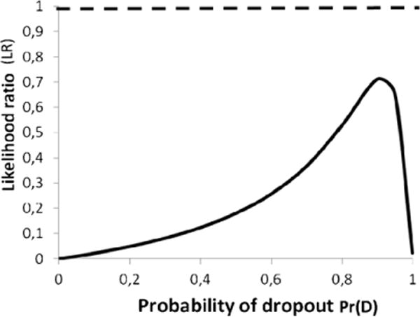
Effect of Pr(D) on LR. Suspect is ab and crime stain evidence is ac. Locus D18S51 allele 13 frequency was used to calculate the LR example (pa = 0.135). Since LR < 1, then this favours Hd. The dashed line indicates LR = 1.
Occasionally, a spurious allele in an otherwise complete DNA profile may occur. Practices to deal with such isolated phenomena vary widely, but it is still common practice in a number of laboratories to leave the locus out of any statistical calculation and, thus estimate that the weight is neutral, i.e. LR = 1. If a calculation based on probabilistic principles indicates that LR < 1, assignation of neutrality to the results of a locus is prosecution biased as Fig. 5 illustrates.
13. Summary of recommendations of the ISFG DNA commission
Probabilistic methods following the ‘basic model’ described here can be used to evaluate the evidential weight of DNA results considering drop-out and/or drop-in.
Estimates of drop-out and drop-in probabilities should be based on validation studies that are representative of the method used.
The weight of the evidence should be expressed following likelihood ratio principles.
The use of appropriate software is highly recommended to avoid hand-calculation errors.
14. Concluding remarks
The recommendations explain how probabilistic approaches and likelihood ratio principles can be applied to partial and potentially compromised DNA profiles. The recommendations concentrate on situations with only one possible drop-in and/or one drop-out. We are aware that the approach described here is based on a number of simplified assumptions that have been made to demonstrate the underlying principles. Furthermore, we are aware that DNA results of ‘real life’ stains do not always fulfil these assumptions (they may e.g. comprise multiple contributors) and will therefore require statistical calculations more complex than those used here. However, the methods can be extended to multiple loci and multiple contributors using ‘set theory’ [5]. The recommendations demonstrate why probabilistic approaches and likelihood ratio principles are superior to classical methods. The combined efforts of the scientific community should be focussed at taking into account the stochastic phenomena that we have all been aware of for many years [10], and to develop interpretation tools that will become generally accepted and used. We do not advocate a ‘black-box’ approach.
The introduction of software solutions to interpret DNA profiles must be accompanied by a validation process ensuring conformity with existing standard laboratory procedures. Validation studies should be carried out to characterise drop-out and drop-in probabilities bearing in mind that these will differ between processes (some guidance is given in the appendices). Open-source is strongly encouraged since this solution offers unrestricted peer review and best assurance that methods are fit for purpose. Internal laboratory policies are necessary in order to address the quality of the data that will be required to attempt a comparative interpretation. Strict anti-contamination procedures must be established to minimise the introduction of any additional levels of uncertainty. Software tools used for casework implementation must be evaluated with known samples and each laboratory will have to establish reporting guidelines and testimony training to properly present the results to courts.
Supplementary Material
Acknowledgments
Peter Gill has received funding support from the European Union Seventh Framework Programme (FP7/2007-2013) under grant agreement n̊ 285487.
Appendix A
A.1. The evolution of the ‘virtual allele’ and its relationship to drop-out theory
A.1.1. The ‘F’ designation
The concept of the virtual allele has existed for many years. The ‘F’ designation was used to signify a potential hidden ‘unknown’ allele. It was applied to an apparent homozygote, where a single present allele was below the ‘stochastic threshold’, and at a level (peak height) where it would be reasonable to assume that dropout might have occurred. This concept gave rise to the 2p × pF rule, where p is the frequency of the observed allele, and pF is the frequency of some (any) unknown allele, where pF= 1, hence F is usually omitted in the expression.
A.1.2. The ‘Q’ designation in the classical model
The ‘Q’ designation was a simple extension of the F designation.
Consider a locus with n alleles such that p1 + … + pn = 1, where pi is the frequency of allele i.
We consider a visualized phenotype a within a stain and a suspect. There is an allele that could have dropped out.
The possible genotypes under Hd (drop-in and drop-out probabilities are not considered here):
No drop-out: homozygote aa,
Drop-out: heterozygote aQ
The LR is:
| (A.1) |
A.1.3. Use of the Q designation in the drop-out model
The probability of drop-out of a homozygote was originally estimated as Pr(D)2 [4]. However, Balding and Buckleton [18] argued that the probability of dropout of a homozygote would be overestimated using this method: “both alleles can generate partial signals that combine to reach the reporting standard, whereas each individual signal would fail to reach this standard,” and suggested an empirical correction factor (α) to compensate. They used an example where alpha was set to 0.5. Using the notation Pr(D2) to signify homozygote dropout, this can be calculated directly from Pr(D):
| (A.2) |
Alternatively, Pr(D2) can be empirically estimated.
This resulted in two drop-out parameters, one for both alleles in a homozygote and one for each allele in a heterozygote.
Eq. (A.1) can be re-evaluated with respect to drop-out probabilities:
If the suspect is ab we require no dropout of allele a, with the probability , and drop-out of allele b, with the probability Pr(D).
Under Hd, if there is no drop-out, the genotype is aa with the probability of . Alternatively, if there is drop-out, the genotype is aQ with the probability of .
Eq. (A.1) now becomes:
| (A.3) |
In example 2 (section 11), we consider the simultaneous possibility of drop-in and drop-out.
In the crime-stain, alleles a and c are observed. The suspect’s genotype is ab. Hence the observed alleles in the crime-stain are a and c, and the Q allele is an unobserved allele that can beany allele not observed in the crime-stain
Under Hp, the suspect is ab, which requires drop-out of allele b and drop-in of allele c.
Under Hd, all of the pairwise combinations of the set of alleles a, c, Q are listed below:
| Putative genotype probability | ||
| aa |
|
|
| cc |
|
|
| ac |
|
|
| aQ |
|
|
| cQ |
|
|
|
|
||
| QQ′ |
|
|
Note that in the last row we introduce QQ′ to signify dropout of a heterozygote locus in addition to QQ that signifies dropout of a homozygote locus, as the formulae (and drop-out probabilities) differ between these two states.
A.1.4. Further explanation of Q and Q′
To continue the example in section 1.3: for illustration purposes only, consider that five alleles (a,b,c,d,e) were observed in a population survey (the principle can be extended to any number of alleles). QQ defines the genotype if a homozygote has dropped out and is associated with the probability of dropout, Pr(D2). As we have already considered the probabilities of aa and cc in the above list in section 1.3, the Q designation is calculated from the frequencies of summed (unobserved) genotypes, and in our five-allele example these are homozygotes bb, dd, or ee. The probability of the QQ genotype is therefore: and the probability of the QQ genotype combined with its probability of dropout is .
pQQ′ defines the probability of heterozygote genotype QQ′ (where neither Q nor Q′ is type a or type c (since we have already evaluated genotypes aQ, cQ in the above list), which corresponds to a heterozygote locus drop-out. Q≠Q′ (because the genotype must be a heterozygote). Therefore, the probability of genotype QQ′ is constructed from the probabilities of unobserved heterozygote genotypes in the population of five-alleles, which are 2pbpd, 2pbpe and 2pdpe:
| (A.4) |
Q′ is always used with Pr(D), hence the combined probability of QQ′ is 2pQpQ′Pr(D)2.
Appendix B
B.1. The logistic model for the estimation of Pr(D)
B.1.1. Experimental design
In order to carry out the estimation of the probabilities of dropout using the logistic model of Gill & Puch-Solis [9], it is necessary to collect data within the range of interest. Laboratories usually have a good understanding of their STR typing systems, and will know the limits of the system, where dropout may occur. Many laboratories use a stochastic threshold (typically 150rfu) where they decide that alleles below this level may be absent. Gill and Puch Solis [9] described a method to calculate thresholds relative to Pr(D). The experiment may be designed, either as a series of dilutions, either of body fluid, or comprised of naked DNA. The latter is usually carried out for practical reasons, but may be subject to the criticism that dilution of naked DNA does not simulate the diploid cell, since the chromosomal associations are destroyed prior to dilution [13].
Considering a heterozygote, there are three outcomes (we use a notation in parentheses where 1 means dropout and 0 means no dropout):
Two alleles are present (0,0);
One allele is present and the other is absent, (1,0) or (0,1);
Both alleles are absent – locus dropout (1,1).
The experiment needs to be designed so that the data produce all three types of events. This is easiest to achieve if the laboratory runs a pilot study in order to determine a range of concentrations of DNA that produce all three states within the same experiment. It is suggested that a sample size of 100 profiles should be sufficient.
Table B.1.
Raw dataset showing allele designation and its recorded peak height (rfu).
| Sample no. | Allele designation | Allele peak height | Allele designation | Allele peak height |
|---|---|---|---|---|
| 1 | 17 | 135 | 25 | 193 |
| 2 | 11 | 30 | 13 | 80 |
| 3 | 29 | 157 | 30 | 160 |
| 4 | 14 | 30 | 16 | 142 |
| 5 | 13 | 319 | 14 | 117 |
| 6 | 6 | 150 | 9.3 | 36 |
| 7 | 21 | 56 | 23 | 30 |
We are interested in the peak heights of the alleles. An allele is deemed to have dropped out if it is below the limit of detection threshold (LDT) of 50rfu (for example). To carry out the experiment, it is useful to lower the detection limit threshold on the sequencing instrument to 30rfu because this extends the curve and improves the Pr(D) estimation below the LDT = 50rfu threshold.
A small subset of seven observed heterozygous loci is shown from a dataset of 496 loci (in total) from a validation exercise of the standard SGM Plus kit (Table B.1):
B.1.2. An explanation of logistic regression
Ordinary linear regression models follow the formula:
Where y is the dependent variable (the drop-out indicator of the allele of interest), and x is the explanatory variable (the height of the partner allele in rfu). Note that y has a linear relationship to x and a and b are the linear model parameters, which can be estimated via simple linear regression.
In the example shown in Table B.1, the dependent variable (y) is binary, either zero or one. In this example, we wish to work out the probability of dropout as our dependent variable. The logistic regression works by calculating odds P/(1−P). For example, suppose we take a subset of data between 125rfu – 175rfu and wish to calculate the odds of dropout, and we carry out experimentation, observing that 25 out of 100 loci do indeed exhibit dropout (Pr = 0.25), we translate this into odds: 0.25/0.75 = 0.33. Conversely, the odds of no drop-out is 0.75/0.25 = 3.
These two numbers are asymmetrical but applying natural logarithm regains the symmetry, since ln(0.33) = −1.099 and ln(3) = 1.099, so now we have symmetry and odds of dropout vs. no dropout are of opposite sign. Taking the natural logarithm of odds is known as the logit function and the logistic regression formula is essentially the same as the linear regression formula, where y = logit Pr(D):
By algebraic rearrangement, we can calculate Pr(D), the probability of dropout as a continuous variable from:
B.1.3. Software
-
1)
Logistic regression is standard in software applications and is very easy to carry out. For example in Matlab, the following code will calculate the regression coefficients and plot a graph. Data are stored in variable ‘AllData’ as arranged in Table B.3 (peak heights need to be sorted in descending order):
[logitCoef,dev] = glmfit (x,y ’binomial’, ’logit’);
logitFit = glmval (logit Coef, x ’logit’);
plot (x, logitFit, ’r−’);
xlabel (’PeakHeight’); ylabel (’Probability’);
-
2)
In the open-source software, R, the following commands are used:
fit = glm(y~x, family = binomial)
summary(fit)
where y is the binomial response and x is the covariate in both examples.
The Matlab output for a validation exercise carried out by Norwegian Institute of Public Health (unpublished) for the SGM plus system, incorporating a total of 495 heterozygote loci from 55 samples is shown in Fig. B.1.
It is informative to plot the logistic regression using log Pr(D) since this gives a straight line relationship and can be used to evaluate the risks at very low probabilities. For example, the risk of dropout if there is a single allele at 250rfu is Pr = 4 × 10⁻⁴. Because we have extended the estimation of the curve to 30rfu, we can comfortably estimate the lower limit of dropout, Pr(D) = 0.45 at the LDT = 50rfu. This is itself interesting, because we can equate the LDT with an expectation about 45% of heterozygote alleles given a surviving partner allele peak height of 50rfu.
Table B.2.
The table has been modified so that now each peak height is associated with a 0 or 1 binary designation to signify the state of the partner allele as either ‘not dropped out’ or ‘dropped out’, respectively.
| Sample no. | Allele designation | Allele peak height | Allele designation | Allele peak height | Drop-out state* |
|---|---|---|---|---|---|
| 1 | 17 | 135 | 25 | 193 | 0 |
| 2 | 11 | 30 | 13 | 80 | 0 |
| 3 | 29 | 157 | 30 | 160 | 0 |
| 4 | 14 | 30 | 16 | 142 | 0 |
| 5 | 13 | 319 | 14 | 117 | 0 |
| 6 | 6 | 150 | 9.3 | 36 | 1 |
| 7 | 21 | 56 | 23 | 30 | 1 |
Drop-out state=0 means no drop-out of companion allele and drop-out state=1 means drop-out is observed. All drop-out states are conditioned on alleles in the fourth/fifth columns.
Table B.3.
Now the data are organised into two columns: peak height and the state of the partner allele. This data is used for logistic regression.
| Sample no. | Allele peak height | Drop-out state* |
|---|---|---|
| 1 | 135 | 0 |
| 2 | 30 | 0 |
| 3 | 157 | 0 |
| 4 | 30 | 0 |
| 5 | 319 | 0 |
| 6 | 150 | 1 |
| 7 | 56 | 1 |
Drop-out state=0 means no drop-out of companion allele and drop-out state=1 means drop-out is observed.
Fig. B.1.

Logistic regression analysis of the probability of drop-out using the SGM Plus kit. E.g., 150 rfu peak height corresponds to Pr(D) = 0.03.
Given the size of the peaks illustrated in Figs. 3–5, these probabilities can be plugged directly into the examples in the text.
B.1.4. Using R code
The following script can be run in R to generate the graph shown in Fig. B.3.
# Prepare data in 2 columns with first column = peak height and column 2=binary response variable
# Save into .csv format and run the code to generate summary statistics and plot
dat<−read.table(file="LogisticTableR.csv",sep=",",header=TRUE)
x=dat[,1]
y=dat[,2]
data1=cbind.data.frame(x,y)
mod1 = glm(y~x, family = binomial,data=data1)
summary(mod1)
plot(x,y,ylab="Probability of dropout",xlab="size (Peak
Height)",xlim=c(0,300),pch=20)
curve(predict(mod1,data.frame(x=x),type="resp"),add=TRUE)
The logistic regression is fundamental to an understanding of dropout. The method is used by e.g. Tvedebrink et al. [14,20].
Finally, we note that the logistic regression model applies to heterozygotes only. The estimation is different for homozygotes, but we do not consider further here since Buckleton [12] showed that under the condition where E is a and S is aa, there is no anticonservative issue with reporting . The issue relates solely to the E being a and S being ab, where anti-conservativeness is a possibility with the 2p rule.
Fig. B.2.

Logistic regression analysis of the probability of drop-out on a log-scale (SGM Plus kit).
Fig. B.3.
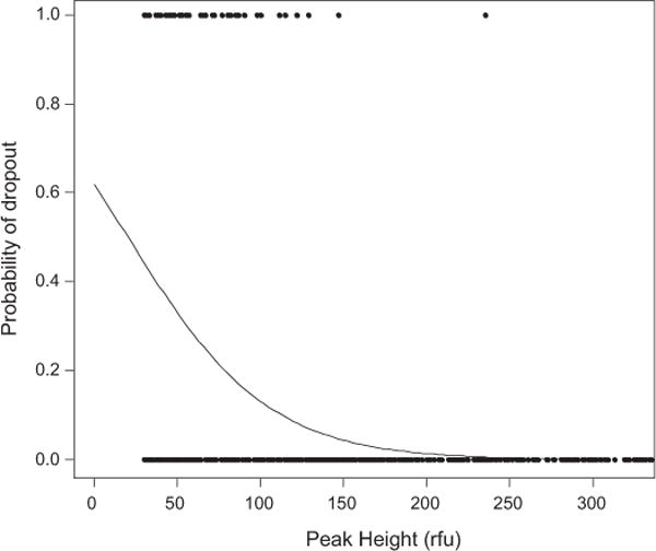
The R-code produces this logistic regression plot. Actual data-points are shown. The figure also shows the raw data points for drop-out and no drop-out respectively. See Curran [19] for detailed examples and tutorials.
Appendix C. Supplementary data
Supplementary data associated with this article can be found, in the online version, at http://dx.doi.org/10.1016/j.fsigen.2012.06.002.
Footnotes
Also known as the homozygote threshold. The level is often determined by experimentation and is set to an arbitrary level where it is highly unlikely that a drop-out event occurs if an allele is above the designated threshold. This enables a homozygote to be designated with a high degree of confidence. If a single allele at a locus appears below the stochastic threshold, it is designated aF, where F signifies that ‘any allele’, including a, may be present. In this paper, we refer to the threshold for convenience. Strictly speaking, thresholds are not needed in the probabilistic framework described. But if used, the threshold can be associated with a ‘risk’ defined in terms of the probability of drop-out.
If a complex DNA profile, such as a mixture, is analysed, then the numerator will often be less than one, but this will usually be because of the uncertainty of the genotype frequency, rather than the uncertainty of the genotype designation. If there is a three-allele profile abc, where the suspect genotype is ab, an unknown contributor is ac, bc or cc, the Hp probability is therefore .
Drop-in rate may increase for mixed samples; enhanced stutters may be classified as drop-in events.
In the probabilistic framework, it would be unusual for any probability to be exactly one or zero since there is always a measure of uncertainty that exists.
Ideally, one random allele per locus is chosen. If both alleles were used in the logistic regression, then they act as both the response and the explanatory variables at the same time. This violates the requirement of independent observations of the logistic regression.
References
- 1.Gill P, Brenner CH, Buckleton JS, Carracedo A, Krawczak M, Mayr WR, Morling N, Prinz M, Schneider PM, Weir BS. DNA Commission of the International Society of Forensic Genetics: recommendations on the interpretation of mixtures. Forensic Sci Int. 2006;160:90–101. doi: 10.1016/j.forsciint.2006.04.009. [DOI] [PubMed] [Google Scholar]
- 2.Morling N, Allen RW, Carracedo A, Geada H, Guidet F, Hallenberg C, Martin W, Mayr WR, Olaisen B, Pascali VL, Schneider PM. Paternity Testing Commission of the International Society of Forensic Genetics: recommendations on genetic investigations in paternity cases. Forensic Sci Int. 2002;129:148–157. doi: 10.1016/s0379-0738(02)00289-x. [DOI] [PubMed] [Google Scholar]
- 3.Gjertson DW, Brenner CH, Baur MP, Carracedo A, Guidet F, Luque JA, Lessig R, Mayr WR, Pascali VL, Prinz M, Schneider PM, Morling N. ISFG: recommendations on biostatistics in paternity testing. Forensic Sci Int Genet. 2007;1:223–231. doi: 10.1016/j.fsigen.2007.06.006. [DOI] [PubMed] [Google Scholar]
- 4.Gill P, Whitaker J, Flaxman C, Brown N, Buckleton J. An investigation of the rigor of interpretation rules for STRs derived from less than 100 pg of DNA. Forensic Sci Int. 2000;112:17–40. doi: 10.1016/s0379-0738(00)00158-4. [DOI] [PubMed] [Google Scholar]
- 5.Curran J, Gill P, Bill M. Interpretation of repeat measurement DNA evidence allowing for multiple contributors and population substructure. Forensic Sci Int. 2005;148:47–53. doi: 10.1016/j.forsciint.2004.04.077. [DOI] [PubMed] [Google Scholar]
- 6.Haned H. Forensim: an open-source initiative for the evaluation of statistical methods in forensic genetics. Forensic Sci Int Genet. 2011;5:265–268. doi: 10.1016/j.fsigen.2010.03.017. [DOI] [PubMed] [Google Scholar]
- 7.Perlin MW, Szabady B. Linear mixture analysis: a mathematical approach to resolving mixed DNA samples. J Forensic Sci. 2001;46:1372–1378. [PubMed] [Google Scholar]
- 8.Curran JM, Triggs CM, Buckleton J, Weir BS. Interpreting DNA mixtures in structured populations. J Forensic Sci. 1999;44:987–995. [PubMed] [Google Scholar]
- 9.Gill P, Puch-Solis R, Curran J. The low-template-DNA (stochastic) threshold–its determination relative to risk analysis for national DNA databases. Forensic Sci Int Genet. 2009;3:104–111. doi: 10.1016/j.fsigen.2008.11.009. [DOI] [PubMed] [Google Scholar]
- 10.Whitaker JP, Cotton EA, Gill P. A comparison of the characteristics of profiles produced with the AMPFlSTR SGM Plus multiplex system for both standard and low copy number (LCN) STR DNA analysis. Forensic Sci Int. 2001;123:215–223. doi: 10.1016/s0379-0738(01)00557-6. [DOI] [PubMed] [Google Scholar]
- 11.Gill P, Curran JM, Elliot K. A graphical simulation model of the entire DNA process associated with the analysis of short tandem repeat loci. Nucleic Acids Res. 2005;33:632–643. doi: 10.1093/nar/gki205. [DOI] [PMC free article] [PubMed] [Google Scholar]
- 12.Buckleton J, Triggs C. Is the 2p rule always conservative? Forensic Sci Int. 2006;159:206–209. doi: 10.1016/j.forsciint.2005.08.004. [DOI] [PubMed] [Google Scholar]
- 13.Haned H, Egeland T, Pontier D, Pene L, Gill P. Estimating drop-out probabilities in forensic DNA samples: a simulation approach to evaluate different models. Forensic Sci Int Genet. 2011;5:525–531. doi: 10.1016/j.fsigen.2010.12.002. [DOI] [PubMed] [Google Scholar]
- 14.Tvedebrink T, Eriksen PS, Mogensen HS, Morling N. Estimating the probability of allelic drop-out of STR alleles in forensic genetics. Forensic Sci Int Genet. 2009;3:222–226. doi: 10.1016/j.fsigen.2009.02.002. [DOI] [PubMed] [Google Scholar]
- 15.Mitchell AA, Tamariz J, O‘Connell K, Ducasse N, Prinz M, Caragine T. Likelihood ratio statistics for DNA mixtures allowing for drop-out and drop-in. Forensic Sci Int Genet (Suppl Ser) 2011;3:e240–e241. [Google Scholar]
- 16.Gill P, Rowlands D, Tully G, Bastisch I, Staples T, Scott P. Manufacturer contamination of disposable plastic-ware and other reagents—an agreed position statement by ENFSI, SWGDAM and BSAG. Forensic Sci Int Genet. 2010;4:269–270. doi: 10.1016/j.fsigen.2009.08.009. [DOI] [PubMed] [Google Scholar]
- 17.Benschop CC, van der Beek CP, Meiland HC, van Gorp AG, Westen AA, Sijen T. Low template STR typing: effect of replicate number and consensus method on genotyping reliability and DNA database search results. Forensic Sci Int Genet. 2011;5:316–328. doi: 10.1016/j.fsigen.2010.06.006. [DOI] [PubMed] [Google Scholar]
- 18.Balding DJ, Buckleton J. Interpreting low template DNA profiles. Forensic Sci Int Genet. 2009;4:1–10. doi: 10.1016/j.fsigen.2009.03.003. [DOI] [PubMed] [Google Scholar]
- 19.Curran JM. Introduction to Data Analysis with R for Forensic Scientists, CRC Press, Taylor and Francis Group. 2011:234–253. [Google Scholar]
- 20.Tvedebrink T, Eriksen PS, Asplund M, Mogensen HS, Morling N. Allelic dropout probabilities estimated by logistic regression–further considerations and practical implementation. Forensic Sci Int Genet. 2012;6:263–267. doi: 10.1016/j.fsigen.2011.06.004. [DOI] [PubMed] [Google Scholar]
Associated Data
This section collects any data citations, data availability statements, or supplementary materials included in this article.