Robust Anatomical Landmark Detection with Application to MR Brain Image Registration

Abstract

Comparison of human brain MR images is often challenged by large inter-subject structural variability. To determine correspondences between MR brain images, most existing methods typically perform a local neighborhood search, based on certain morphological features. They are limited in two aspects: (1) pre-defined morphological features often have limited power in characterizing brain structures, thus leading to inaccurate correspondence detection, and (2) correspondence matching is often restricted within local small neighborhoods and fails to cater to images with large anatomical difference. To address these limitations, we propose a novel method to detect distinctive landmarks for effective correspondence matching. Specifically, we first annotate a group of landmarks in a large set of training MR brain images. Then, we use regression forest to simultaneously learn (1) the optimal sets of features to best characterize each landmark and (2) the non-linear mappings from the local patch appearances of image points to their 3D displacements towards each landmark. The learned regression forests are used as landmark detectors to predict the locations of these landmarks in new images. Because each detector is learned based on features that best distinguish the landmark from other points and also landmark detection is performed in the entire image domain, our method can address the limitations in conventional methods. The deformation field estimated based on the alignment of these detected landmarks can then be used as initialization for image registration. Experimental results show that our method is capable of providing good initialization even for the images with large deformation difference, thus improving registration accuracy.

1. Introduction

Accurate matching of anatomical structures is a key step in many medical image processing and analysis tasks, e.g., deformable image registration (Zacharaki et al., 2008, 2009; Xue et al., 2006; Zhan et al., 2006; Shen et al., 1999), organ motion correction (Castillo et al., 2010), and imaging biomarker identification (Zhang et al., 2011; Fan et al., 2007; Wee et al., 2011; Chen et al., 2009). For example, the goal of deformable image registration is to maximize the image similarity by spatially warping one image to another. To achieve this, accurate determination of matching structures between images is crucial. Correspondence detection can be achieved by using either image intensities or image features (e.g., SIFT (Lowe, 1999), geometric invariant moments (Shen and Davatzikos, 2002), and wavelet transformation (Xue et al., 2004)).

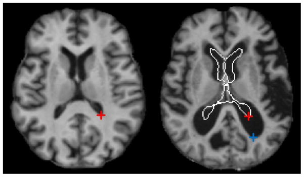
However, anatomical structures can vary significantly across individuals. For instance, as shown in Fig. 1, the brain images from two individuals can differ significantly in ventricle size and their corresponding structures (i.e., marked by the red and blue crosses). Large structural differences pose huge challenges for accurate and robust correspondence detection. Current methods typically perform a local neighborhood search to find anatomical correspondences between images, by comparing the similarity between a target landmark in one image and all nearby candidate points in another image (Xue et al., 2004; Wu et al., 2006; Shen, 2009; Yang et al., 2008). Such approach is limited in two aspects: (1) Current methods neglect the fact that, due to large inter-subject variability, corresponding structures could be far away and also exhibit different appearances, thus leading to inaccurate matching. (2) The similarity between corresponding points is often measured using local image features (e.g., intensity or SIFT features), rather than global image information that can help better distinguish between structures. Moreover, the same feature is usually used for the entire image -- this fails to take into account the structural variation within an image. We propose two ways to improve correspondence detection: (1) design discriminative feature descriptors that can enhance uniqueness in correspondence detection, and (2) use a global correspondence detection mechanism that can deal with the large anatomical difference between individual subjects.

Fig. 1.

An example showing the large difference between ventricular regions in the two MR brain images. The boundary of ventricular region in the left image is overlaid on the right image. The red and blue cross marks denote the reference and the corresponding points in the two images, respectively. The distance between two cross marks in the right image is about 19mm.

In this paper, we propose a supervised global anatomical landmark detection method for MR brain images, which can address the aforementioned limitations in correspondence detection. More specifically, for each landmark, a robust correspondence detector is learned using a regression forest, an ensemble of randomly-trained binary decision trees that can efficiently map a complex input space to continuous output parameters (Criminisi et al., 2011a). The highly non-linear mappings are solved by converting the original complex problem into a set of small-scale problems that can be handled with simple predictors. Regression forest has been proved to be a powerful tool for a variety of learning tasks (Criminisi et al., 2011a, 2011b; Pauly et al., 2011; Donner et al., 2013; Lindner et al., 2013). In our proposed method, regression forest is used to efficiently predict the pathways from all possible points in a new MR brain image to the corresponding landmark. More specifically, in the training stage, we annotate a set of salient landmarks, corresponding to the common anatomical structures, in a number of training MR brain images. Then, a regression forest is employed to simultaneously learn the optimal set of features that can best characterize these landmarks and also the complex non-linear mappings from local patch appearances of an image to these landmarks. In the application stage, the trained regression forest is used to predict the displacements of each point in a new image towards a corresponding landmark. Based on the predicted displacements, a “point jumping” strategy is proposed to determine the location of the landmark, which is shown to be more robust than the simple majority-voting approach when there is large anatomical structure variation. Robustness and efficiency of landmark detection is further improved by adopting a multi-resolution implementation. Because landmark detection is performed in the entire image domain, our proposed method is able to handle the challenge of large structure variations. Moreover, since a unique detector is learned for a specific anatomical landmark, more discriminative features could be utilized to best distinguish a landmark from other points in the MR brain image.

To evaluate the performance of our multi-resolution regression-guided landmark detection method, we apply it to MR brain image registration for addressing the problem of registering images with large anatomical differences. For computational efficiency, we first select a small set of landmarks that are sparsely covering the whole brain. Then, a unique detector is learned for each landmark by using regression forest. These detectors are used to establish rough initial correspondences between two MR brain images. Further refinement of the initial deformation field can be performed by using a registration algorithm, e.g., the HAMMER algorithm (Shen and Davatzikos, 2002), which is one of the state-of-the-art feature-based deformable registration methods. Experimental results show that these learned landmark detectors are quite robust to large anatomical variability among subjects. After landmark-based initialization, inter-subject differences are significantly reduced, thus making the subsequent registration-based refinement much easier. In our experiments, more accurate and robust results are obtained by combining these landmark detectors with HAMMER, especially for the cases with large anatomical differences.

The preliminary version of this work was published in (Han et al., 2014). But this work differs from our previous work in the following aspects. 1) More detailed descriptions of the method are presented. Also, an algorithm (Alg. 1) also given for readers to better understand the detailed implementation of our point-jumping landmark detection method. 2) Comprehensive parameter setting is provided in Section 3, which makes it feasible to reproduce our results by others. 3) Experimental Section is extensively extended with more visual results and also a validation on additional “18-elderly-brain” dataset.

This paper is organized as follows. In Section 2, we describe the multi-resolution regression-guided anatomical landmark detection method and its application to MR brain image registration. Evaluation results of the proposed method are presented in Section 3. Finally, we conclude this paper in Section 4.

2. Methods

In this section, we first introduce the training and application procedures of general regression forest in Subsection 2.1. Then, in Subsection 2.2, we give the detailed descriptions of our multi-resolution regression-guided landmark detection method. Finally, in Subsection 2.3, we describe the application of using our proposed method to assist MR brain image registration.

2.1 Regression forest

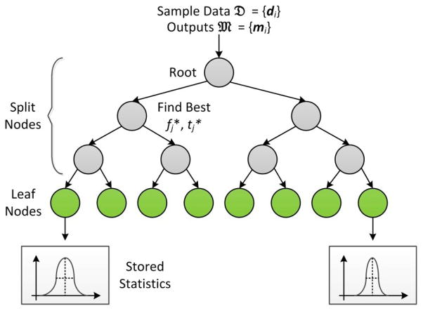
In multivariate regression, we want to learn a mapping that predicts a continuous output m ∈ ℝ^M using input d ∈ ℝ^D. Regression forest belongs to random forest family and is specialized for non-linear regression. A regression forest consists of a set of binary decision trees. Each binary decision tree contains a number of split and leaf nodes as shown in Fig. 2. A split node is associated with a split function, which directs an incoming data item to either left or right child based on a single feature and the learned threshold; on the other hand, a leaf node stores a statistical distribution of outputs of training data items that fall into it. This piece of information would be used to determine the output of an unseen testing data item. In this paper, a training data item consists of data extracted at a point of a training image (i.e., training point), d ∈ ℝ^D is a vector that contains image features calculated from the local patch centered at the training point, and m ∈ ℝ^M (M = 3) is the 3D displacement from this training point to an annotated landmark. In the next two paragraphs, we will briefly introduce (1) in the training stage how regression forest is learned to capture the non-linear relationship between d and m, and (2) in the application stage how the learned forest is used to predict the output of an unseen data item.

Fig. 2.

A simple example of a four-level binary decision tree in a regression forest. Gray and green nodes are split nodes and leaf nodes, respectively.

In the training stage, each tree is trained independently, and thus training can be performed in parallel. Given a set of sampled training data items = {d_i ∈ ℝ^D, i = 1 ··· N} and their corresponding continuous outputs = {m_i ∈ ℝ^M, i = 1 ··· N}, the training of a binary decision tree starts with the root node, and recursively proceeds to its left and right children until either of the two stopping criteria is met: (1) the maximum tree depth D_Tree is reached; (2) the number of training data items after splitting is below a threshold N_Leaf. If none of the two stopping criteria is met, the current node is a split node; otherwise, it is a leaf node. For each split node j, we want to find the optimal feature $f_j^{\ast }$ and threshold $t_j^{\ast }$ that best split the training data items into two groups with consistent output values {m_i}. This is typically done using exhaustive search over a random feature and threshold set by maximizing the following objective function:

$$\begin{array}{c}{\text{objective}}_j(f,t)=\mathrm{E}({\mathbf{\Omega }}_j)-\frac{\mid {\mathbf{\Omega }}_j^{\mathrm{L}}\mid }{\mid {\mathbf{\Omega }}_j\mid }\mathrm{E}({\mathbf{\Omega }}_j^{\mathrm{L}})-\frac{\mid {\mathbf{\Omega }}_j^{\mathrm{R}}\mid }{\mid {\mathbf{\Omega }}_j\mid }\mathrm{E}({\mathbf{\Omega }}_j^{\mathrm{R}})\\ {\mathbf{\Omega }}_j^{\mathrm{L}}=\{i\in {\mathbf{\Omega }}_j\mid f({\mathit{d}}_i)\le t\},{\mathbf{\Omega }}_j^{\mathrm{R}}=\{i\in {\mathbf{\Omega }}_j\mid f({\mathit{d}}_i)>t\}\\ \mathrm{E}({\mathbf{\Omega }}_j)=\text{trace}(cov({\mathfrak{M}}_{{\mathbf{\Omega }}_j}))\end{array}$$

where f and t denote a pair of randomly sampled feature and threshold, Ω_j denotes the index set of training data items that arrive at node j, Objective_j(f, t) measures how well a particular pair of feature and threshold separates the training data set indexed by Ω_j into two groups with consistent outputs, ${\mathbf{\Omega }}_j^{\mathrm{L}}$ and ${\mathbf{\Omega }}_j^{\mathrm{R}}$ are the index sets of training data items that arrive at left and right children of node j after splitting, respectively, E(Ω_j) computes the consistency of output values of training data set indexed by Ω_j, f(d_i) returns the response of feature f on data item d_i, denotes the outputs of training data items indexed by Ω_j, trace denotes the matrix trace, and cov denotes covariance matrix. After determining the optimal feature and threshold, we split the training data items into two groups, which are further passed to the left and right children for training, respectively. For each leaf node, we can save the posterior probability p(m|d) by summarizing the outputs of all training data items that arrive at this leaf. In most cases, by assuming Gaussian distribution of outputs in each leaf, only mean and covariance of outputs need to be calculated. The entire tree training continues until all training paths reach the leaves.

In the application stage, we can use the learned regression forest to predict the output of an unseen data item d_new ∈ ℝ^D. Similar to the training stage, the prediction of each binary decision tree is independent, and also can be performed in parallel. To predict the output of d_new from one binary decision tree, we push data item d_new through the tree starting at the root. At each split node j, we compute the feature response $f_j^{\ast }({\mathit{d}}_{\text{new}})$ and compare it with threshold $t_j^{\ast }$. If $f_j^{\ast }({\mathit{d}}_{\text{new}})\le t_j^{\ast }$, data item d_newis passed to the left child; otherwise, it is passed to the right child. The data item d_new continues being passed until it reaches a leaf node. Under this scenario, the posterior probability distribution p(m|d) saved at that leaf node is used to compute the expectation of m as the output of this tree.

$${\mathit{m}}_k=\int \mathit{m}\ast p_k(\mathit{m}\mid \mathit{d})\mathrm{d}\mathit{m}$$

where m_k is the prediction of the k-th tree, and p_k(m|d) denotes the posterior probability distribution of the leaf node reached by d_new in the k-th tree. The final prediction of a regression forest is computed as the average over predictions of all trees in the forest:

$${\widehat{\mathit{m}}}_{\text{new}}=\frac{1}{K}\sum _{k=1}^K{\mathit{m}}_k$$

Here we assume p(m|d) to be multivariate Gaussian distribution. Thus, the expectation can be efficiently calculated.

2.2 Multi-resolution regression-guided landmark detection

In this paper, regression forest is used as landmark detector to detect the corresponding landmarks across different subjects. In particular, we first use regression forest to simultaneously learn the optimal set of features that best characterize the underlying landmark and a complex non-linear mapping that associates the local patch appearance of an image point with its 3D displacement to the landmark. Then, the learned regression forest is used to detect the latent corresponding landmark in the new testing image by predicting the pathways from the image points to the landmark. Unlike traditional correspondence detection, which is usually performed by feature matching in a small local neighborhood, our regression-guided landmark detection searches for the corresponding landmark in the entire image domain with the automatically learned features. Thus, it is able to overcome large inter-patient anatomical variability. Besides, a unique detector is trained for each landmark of interest under supervised learning setting. Thus, compared with pre-defined features, more discriminative features could be used to best distinguish the underlying anatomical landmark from other points in the MR brain image. In the following paragraphs, we will elaborate the proposed multi-resolution regression-guided landmark detection, from both training and application perspectives.

Training

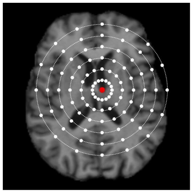
In the stage of detector training, the training dataset consists of a set of linearly aligned MR brain images {I_j}. Each image is associated with the annotated location of a corresponding landmark {v_j ∈ ℝ³}. For each image, we first sample a set of training image points P_Train = {p_i ∈ ℝ³} around the landmark by using spherical sampling as shown in Fig. 3. Specifically, we sample the same number of training points on spheres with different radiuses centered at v_j. Here, the maximum sampling radius is denoted as R_s. More training points are sampled near the annotated landmark, thus the prediction reliability and accuracy of image points close to the landmark can be improved. For the i-th training point ${\mathit{p}}_i^j$ in the j-th training image, its output vector ${\mathit{m}}_i^j\in {ℝ}^3$ is defined as the 3D displacement from this point to the annotated landmark, i.e., ${\mathit{m}}_i^j={\mathit{v}}_j-{\mathit{p}}_i^j$. The features used to characterize each image point are Haar-like features that are computed from a local patch centered at each point, and are defined as follows:

$$\begin{array}{l}\mathrm{\Phi }(\rho )=\sum _{l=1}^z{u}_{l}R(\rho ,{\mathit{a}}_l,s_l)\\ R(\rho ,\mathit{a},s)=\sum _{{\Vert \mathit{q}-\mathit{a}\Vert }_{\infty }\le \frac{1}{2}s}\rho (\mathit{q})\end{array}$$

where ρ is an intensity patch; R(ρ, a_l, s_l) is a cubic function, which calculates an intensity summation over one cubic area within patch ρ; u_l ∈ {−1,1}, a_l ∈ ℝ³ and s_l are the polarity, translation and size parameters of the l-th cubic function, respectively; Z is the number of 3D cubic functions; q is a voxel within patch ρ and ρ(q) is the intensity value of q. By changing the number of 3D cubic functions (i.e., Z) and the parameters of each 3D cubic function (i.e., u_l, a_l and s_l), we can generate virtually unlimited features from an intensity patch ρ. All features that can be represented by Φ(ρ) form the feature pool. When training a binary decision tree, we randomly sample a subset of features F = (f_k, k = 1 ··· N_F} from the feature pool. At each split node, we randomly generate one set of thresholds ${\mathit{T}}_k=\{t_n^k,n=1\cdots N_{\mathit{T}}\}$ for each feature f_k based on the distribution of feature responses of the training image points reaching this node. The feature set F and the corresponding threshold sets {T_k}are used to learn the optimal parameters for split nodes.

Fig. 3.

A sketch diagram of spherical sampling in the training image. The red dot denotes the annotated landmark and the white dots denote the sampled image points. More points are sampled near the annotated landmark so that the prediction reliability and accuracy of image points close to the landmark can be improved.

After defining the sampling strategy, features, and the output that we want to predict, we can train multiple binary decision trees to form a regression forest, which encodes the non-linear relationship between local patch appearance of an image point and its 3D displacement to the landmark.

Testing

In the application stage, the learned regression forest is used to detect the location of corresponding landmark in a new testing image. To achieve it, the most intuitive way is to adopt the idea of “point voting”. In the “point voting”, we allow each image point to vote for the latent landmark location. Specifically, for each image point p ∈ ℝ³, we first predict the 3D displacement vector m̂ ∈ ℝ³ using the learned regression forest, based on the image appearance of the local patch. Then, a vote is given to the point nearest to p + m̂. Finally, after voting from all image points, the point that receives the most votes is regarded as the corresponding landmark location. However, the major limitation of such voting strategy is that the landmark location is determined by consensus of all image points. If large anatomical variations exist near the landmark, majority of image points far away from the landmark would not be informative for landmark prediction. Thus, their prediction results are not reliable. Unfortunately, in the voting strategy, the final landmark location may be dominated by the wrong votes. In our experiments, we will show some cases where the voting strategy fails due to the large inter-subject anatomical structure variations.

In this paper, we propose a regression-guided method for landmark detection, which employs an improved strategy named “point jumping” to overcome the limitations of the voting-based approach. Similar to the “point voting”, each image point can predict one landmark location. The difference is that, instead of directly using the estimated 3D displacement from an image point to predict the landmark, we repeatedly utilize the learned regression forest to estimate a pathway from an image point to the latent landmark, and during this procedure the landmark prediction is iteratively refined. Specifically, given the initial location of an image point p ∈ ℝ³, we can estimate its 3D displacement m̂ to the latent landmark by the learned regression forest. Then, we let this point jump to the new location p + m̂. This “point jumping” procedure continues until it reaches one of the four stopping criteria as stated below:

1. ||m̂|| is too small, which indicates the point does not move anymore and the “point jumping” procedure converges.

2. The currently predicted ||m̂|| is significantly larger than the previously predicted one. In most cases, the point would be very close to the landmark after one jump. The length of jumping should gradually decrease as the point approaches the landmark. This situation happens only when the prediction of ||m̂|| is wrong, and thus the point should stop jumping.

3. The point jumps out of the image domain.

4. The maximum number of jumping is reached.

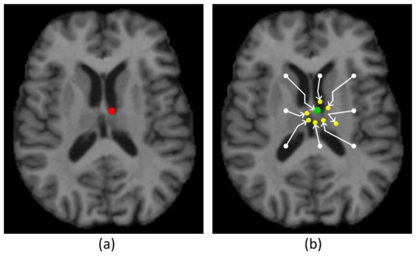
After jumping, the final location of the point is regarded as the predicted landmark location from this point. Given a set of image points, we can use “point jumping” to obtain one predicted landmark location from each point. Then, the predicted location with the smallest ||m̂|| is regarded as the location of the latent landmark. Fig. 4 gives a simple illustration of the “point jumping” strategy. Because the prediction from each point is iteratively refined via “point jumping”, a small set of sampled image points is generally enough for successful landmark detection, which makes this approach much more efficient than “point voting”. In the next paragraph, we will detail the multi-resolution landmark detection and how the image points are sampled in each resolution in the application stage.

Fig. 4.

A sketch diagram of the “point jumping” strategy. The red dot in (a) denotes the true landmark location, the white dots in (b) denote the initial locations of the points, and the green and yellow dots in (b) denote the locations of the points after jumping. The green dot is the final predicted landmark location.

Multi-resolution

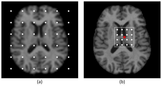
To further increase the robustness of our landmark detection method, we adopt multi-resolution strategies in both training and application stages. Specifically, in the training stage, we train one regression forest for each resolution. In the coarsest resolution, we sample the training points all over the image in order to ensure the robustness of the detector (i.e., large maximum sampling radius in Fig. 3); in the finer resolutions, we only sample the training points near the annotated landmark to increase the specificity of the detector (i.e., small maximum sampling radius in Fig. 3). During the application stage, in the coarsest resolution we sparsely and uniformly sample a set of points from the entire image as shown in Fig. 5(a). Using the “point jumping” on these sampled points, we can obtain an initial guess of the latent landmark. In a finer resolution, we take the predicted landmark in the previous resolution as the initialization. Instead of sampling in the entire image domain, now we sample points only near the initialization (Fig. 5(b)), thus improving the specificity of landmark detection. In this way, the detected landmark will be gradually refined from coarse to fine resolutions. Alg. 1 summarizes our multi-resolution regression-guided landmark detection method.

Fig. 5.

The image point sampling strategies for the coarsest resolution (a) and a finer resolution (b), respectively, in the application stage. For the coarsest resolution, a set of grid points (white dots in (a)) are sampled from the entire image. For a finer resolution, grid points (white dots in (b)) are sampled only near the predicted landmark location (red dot in (b)) from the previous resolution.

Algorithm 1.

Multi-resolution regression-guided landmark detection

Input: An unseen MR brain image I

A set of learned regression forests {Fi} at different resolutions

Notations: ρp denotes a local patch centered at image point p

F(ρp) returns a predicted 3D displacement by forest F based on the local patch ρp

Output: Detected landmark location l

Init: l = the image center of I

for i from the coarsest scale index to the finest scale index do

Uniformly and sparsely sample a set of testing points PTest = {pj} within the bounding box indexed by l − bi/2 and l + bi/2, as shown in Fig. 5. (Here, bi is the side-length vector of the bounding box Bi at resolution i, which gradually decreases as the resolution goes from coarse to fine.)

for each point pj in PTest do

count = 0, p = pj; L = +Inf

while count ≤ MAX_JUMP do

if ||Fi(ρp)|| ≤ TLen then break; endif

if L − ||Fi(ρp)|| ≤ ε then break; endif

if p + Fi(ρp) outside of image domain then break; endif

L = ||Fi(ρp)||; p = p + Fi(ρp); count = count + 1

end while

pj = p

end for

l = argminp∈PTest||Fi(ρp)||

end for

Output: l

In the above, TLen is the threshold for controlling the minimum length for landmark jumping; ε enforces the length of point jumping to be decreasing with some toleration, and ε is usually set to a negative value close to 0.

Summary

Compared with the conventional correspondence detection methods, our method detects the latent landmark in the entire image domain, thus overcoming the limitation of local feature matching and the difficulty of choosing the search range as often suffered by the conventional approaches. Besides, unlike the voting-based landmark detection, we use “point jumping” to iteratively refine the predictions from the image points, which makes our method more accurate under the scenario of large inter-subject structural differences.

2.3 Application of the proposed method to MR brain image registration

In this paper, we demonstrate the advantages of our multi-resolution regression-guided landmark detection method by applying it to MR brain image registration. As shown in Fig. 1, large inter-subject differences pose challenges to accurate correspondence identification. In general, current deformable registration algorithms are limited in solving this problem for two reasons: (1) most deformable registration algorithms adopt a local correspondence matching mechanism, which limits their ability to deal with the large inter-subject anatomical variations; (2) the lack of global image information makes hand-crafted feature descriptors not discriminative enough to identify each point in the brain. Fortunately, our proposed landmark detection method can help alleviate these difficulties.

Ideally, to apply our proposed method to MR brain image registration, we can learn a large number of detectors that are densely distributed in the whole brain. For typical MR brain images, thousands of landmark detectors are often needed to better model the high-dimensional deformation field between two images, which is unfortunately computationally infeasible. To resolve this issue, we select an alternative way. Specifically, we learn a relatively small set of landmark detectors (located at distinctive brain regions) to provide robust initial correspondences between two images. Then, a dense deformation field can be interpolated from the initial correspondences on the landmarks, and is then used to initialize the deformable image registration. Since the most important and challenging correspondences can be well established by our landmark detectors, the subsequent refinement of deformation field becomes much easier than the direct registration between two images. In this way, the conventional image registration can be divided into two sub-tasks, i.e., (1) accurate initial correspondence establishment by robust landmark detectors and (2) efficient deformation refinement by an existing image registration method. Next, we will describe the landmark-based initialization method in detail.

In the stage of detector training, given a group of training MR brain images, we annotate a small set of corresponding landmarks in each image. These landmarks should satisfy two criteria: (1) distinctiveness: a good landmark should be distinctive in terms of its appearance, in order to make the correspondence as reliable as possible; and (2) coverage: the distribution of landmarks should cover the entire brain, in order to effectively drive the whole deformation field. After landmark annotation, a unique detector is learned for each landmark by using the method described in Subsection 2.2.

When registering two new MR brain images, landmark detection is first performed in each image using the learned landmark detectors. Then, sparse correspondences can be established between the two images based on the detected corresponding landmark pairs. Occasionally, a landmark may be incorrectly detected, e.g., at a different region that is too far from its true location. In this case, this landmark together with its corresponding landmark in the other image must be discarded. Recall that we know the exact locations of all the landmarks in the training images, which can be considered as valuable a priori information. Therefore, we can first calculate the average location of each landmark based on the corresponding landmark locations in all training images (after their linear alignment). Then, a simple way to remove the outliers is to calculate the distance between each detected landmark and its corresponding average landmark from the training set. If the distance is larger than a pre-defined threshold, this landmark is considered to be incorrectly detected and is therefore discarded. Next, thin plate spline (TPS) method can be utilized to interpolate a dense initial deformation field from these sparse correspondences (Wu et al., 2010). The generated initial deformation field will be further refined by other deformable registration methods. Since our proposed landmark detection method can provide good initialization for image registration, we can obtain more accurate registration results than directly registering two images from scratch.

3. Experiments

In this section, experiments are conducted to evaluate the performance of the multi-resolution regression-guided landmark detection method. Subsection 3.1 describes the MR brain image datasets used in the experiments and presents the parameter setting for the proposed method. In Subsection 3.2, the proposed method is validated and its advantages are demonstrated. In Subsection 3.3, the proposed method is applied to MR brain image registration to improve the registration accuracy. Experimental results show the advantages of the proposed landmark detection method.

3.1 Image datasets and parameter setting

Two image datasets were used in our experiments. One consisted of 62 MR brain images selected from the ANDI dataset (denoted as the “ADNI dataset”). The other one consisted of 18 MR elderly brain images (denoted as the “18-Elderly-Brain dataset”). The dimensions of these images are 256×256×256, and the voxel size is 1×1×1mm. All these images were first linearly aligned using FLIRT in the FSL software package (Jenkinson and Smith, 2001; Jenkinson et al., 2002). Then, each image was further segmented into white matter (WM), gray matter (GM), ventricle (VN), and cerebrospinal fluid (CSF) regions by FAST (Zhang et al., 2001). Here, we regard these segmentations as the ground truth for evaluating the accuracy of the registration results by comparing the tissue overlap ratio (see Subsection 3.3). To learn a landmark detector, regression forest training was performed on 3 different image resolutions. Table 1 lists the parameter values used in the proposed landmark detection method. The same set of parameters was used in all experiments below.

Table 1.

List of parameters used in the proposed landmark detection method. The same set of parameters was used in all experiments.

Parameters	Coarse resolution	Medium resolution	Fine resolution
K: number of trees	10
DTree: maximum tree depth	12
NF: number of random features per tree	1,500
NT: number of random thresholds per feature	1,000
NLeaf: minimum number of data items in leaf node	10
Rs: maximum sampling radius in training image (mm)	160	80	40
|PTrain|: number of sampled points per training image	6,000
Size (B): size of sampling bounding box in testing image (mm)	200×200×200	100×100×100	50×50×50
|PTest|: number of sampled points in testing image	125
Size(ρ): patch size (in voxels)	30×30×30
s: side length of cubic area within the patch (in voxels)	{3, 5}
Z: number of cubic functions per feature	{1, 2}
MAX_JUMP: maximum number of point jumping	10
TLen: minimum length of point jumping (in voxels)	0.5
ε: minimum decrease in length of point jumping with tolerance (mm)	−2

3.2 Validation of the proposed method

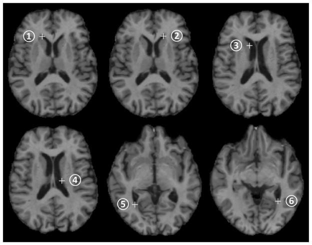
In this subsection, the performance of the proposed landmark detection method is quantitatively and qualitatively evaluated by training detectors for a few specified landmarks and comparing the detection results with the manually annotated landmark locations in the testing images. Specifically, in this experiment, 44 images were selected from the ADNI dataset as the training set and the rest 18 images in the ADNI dataset formed the testing set in the application stage. Next, we manually annotated 6 specific landmarks on the corners/edges of the ventricle regions in both training and testing images. Fig. 6 shows the 6 annotated landmarks in one training image. Then, one detector was trained for each of the 6 landmarks by using the method described in Subsection 2.2.

Fig. 6.

The six manually annotated landmarks on the corners/edges of the ventricular region in one training image. The white crosses mark the landmark locations.

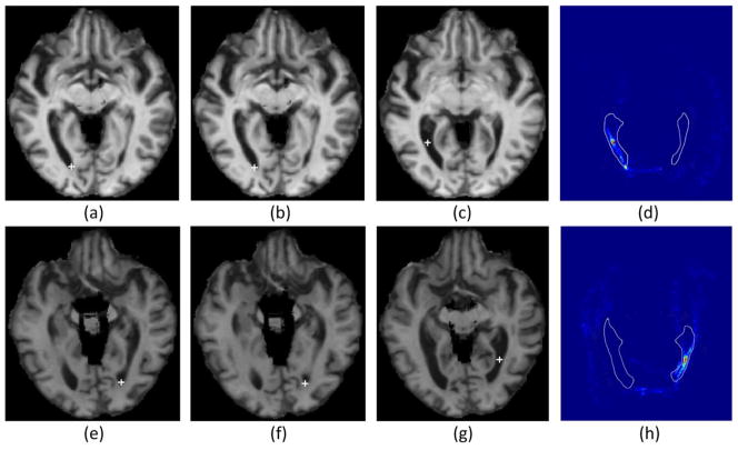
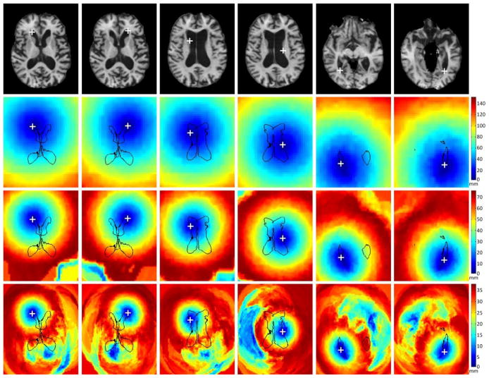
After training, these learned detectors were used to detect the corresponding landmarks in each testing image. The detection results were compared with the annotated landmark locations. To better demonstrate the advantage of the proposed method over the voting-based method, detection results from both methods were obtained and compared. Table 2 presents the detection errors (the residual distance between the manually annotated landmark and the predicted landmark) of the two methods for each of the six landmarks. Both mean errors and corresponding standard deviations are provided. We can obverse from the table that, for the first four landmarks, both methods achieve reasonable detection accuracy with good stability (see the small standard deviations). However, for landmarks 5 and 6, the performance of the voting-based method is far worse than that of the proposed method. This is mainly because the inter-subject variability of these two landmarks is much larger than that of the other four landmarks. In this case, the prediction from the voting-based method is more likely to be dominated by the wrong votes, which eventually leads to false landmark detection. Fig. 7 shows two examples where the voting-based method fails to predict the correct landmark locations, whereas the proposed method still performs well. To better evaluate the performance of the proposed method, we select one image from the testing set that is substantially different in appearance from the training image in Fig. 6. Fig. 8 shows the six annotated landmarks in this image and the corresponding distance maps for each landmark at different resolutions, which are obtained by calculating the distance between each point in the image and the latent landmark based on the regressed displacement from the learned regression forest. From Fig. 8, we can clearly see that, in the coarsest resolution, a rough initial guess of the latent landmark can be robustly estimated from the entire image by the proposed method. This initial prediction is gradually refined in the successive finer resolutions. In this example, all six landmarks are correctly predicted in the finest resolution. Since our proposed method performs landmark detection in the entire image domain, it is not sensitive to anatomical structure variations among different subjects, and thus more robust than its local-search-based counterparts.

Table 2.

The respective detection errors of the voting-based and our proposed detection methods. Both mean errors and corresponding standard deviations are shown. (Unit: mm)

Landmark #	1	2	3	4	5	6
Voting-Based	2.69±1.14	1.94±1.15	2.36±1.21	1.38±0.93	8.60±9.25	5.38±4.94
Proposed	2.62±1.26	2.40±1.08	1.73±1.29	1.48±0.77	2.34±1.53	2.77±1.24

Fig. 7.

Two examples where the voting-based method fails to predict the correct landmark locations, whereas the proposed method still performs well. (a) and (e) are the two images selected from the testing set, along with their manual landmarks 5 and 6; (b) and (f) show the automatically detected landmarks by using the proposed method; (c) and (g) show the detected landmarks by using the voting-based method, with their corresponding voting maps for the two landmarks shown in (d) and (h), respectively, where the white ventricular contours are provided as references for better comparing across images.

Fig. 8.

The six annotated landmarks in one testing image (first row) and their corresponding distance maps at 3 different resolutions (the remaining 3 rows: from coarse to fine resolutions). The white crosses mark the locations of the annotated landmarks. The distance maps are obtained by calculating the distance between each image point and the latent landmark based on the regressed displacement from the learned regression forest.

3.3 Evaluation of the proposed method in MR brain image registration

In this subsection, the proposed landmark detection method was further evaluated by applying it to assist MR brain image registration, where a set of landmark detectors were learned to provide a good initial deformation field between two images under registration. Further refinement of the remaining deformation field was performed by HAMMER (Shen and Davatzikos, 2002), which is one of the state-of-the-art feature-based deformable registration algorithms.

3.3.1 ADNI dataset

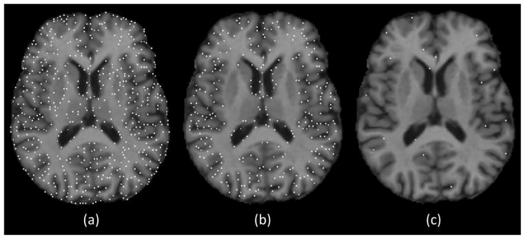
The first group of experiments was conducted by using the ADNI dataset. The same training and testing sets as in Subsection 3.2 were used here. Prior to the training of landmark detectors, we need to select a set of distinctive landmarks that sparsely cover the whole brain. To speed up the procedure of landmark selection, a semi-automatic approach was adopted in our experiment. Specifically, one image in the training set was selected as the template. Then, a large number of candidate landmarks were extracted from the template. This was realized by using the importance sampling strategy described in Wu et al. (2013). Specifically, we first calculated the gradient magnitude at each voxel of the template image. The resulting gradient magnitude map was then smoothed and normalized to serve as the sampling probability map. A voxel with large gradient magnitude indicates its importance and thus has higher probability to be selected as a candidate landmark. The advantage of this sampling strategy is that the extracted candidate landmarks cover the whole brain, especially texture-rich regions. Fig. 9 (a) shows the initially extracted candidate landmarks. Next, we removed the candidate landmarks that were in homogeneous regions (e.g., white matter), because these landmarks are not associated with distinct texture information and may not be reliably detected by regression forest. This was done by first calculating the saliency of each candidate landmark, which is defined as the sum of gradient magnitudes within a small spherical neighborhood. Then, thresholding was performed on these saliency values. Landmarks with saliency values lower than a pre-defined threshold were discarded. Fig. 9 (b) shows the candidate landmark locations after non-salient point removal. Next, we selected a small set of landmarks of interest from all remaining candidate landmarks. This was realized by sorting the candidate landmarks in descending order according to their saliency values, and sequentially picking the final landmarks one by one. Once a candidate landmark was selected as the final landmark, we used a spherical mask centered at the selected landmark to mask out its nearby region. In this way, we could ensure that the selected landmarks evenly covered the whole brain. The landmark selection continued until all candidate landmarks were processed (i.e., either selected or excluded). Fig. 9 (c) shows the final landmarks. In our experiments, 1,350 landmarks were finally selected. Next, we non-rigidly warped all other training images to the template. Based on the deformation fields, the corresponding locations of the landmarks in other training images could be obtained. Because deformable registration may not be accurate enough for each image, we visually checked all the corresponding landmarks and made some necessary corrections to ensure that they all corresponded to the same anatomical structures.

Fig. 9.

Semi-automatic landmark selection strategy. The white dots denote the landmark locations. (a) The initially extracted candidate landmarks. (b) The remaining landmarks after removing the non-salient landmarks. (c) The finally selected landmarks.

After training all the landmark detectors, these detectors were used to establish rough initial correspondences between the two images. Two different cases were considered in this experiment. Case 1 is where the fixed image comes from the training set. This is possible when the training images are used as standard atlases for the applications such as atlas-based segmentation. In this case, landmarks need to be detected only in the new moving image, since the corresponding landmarks in the fixed image are already known. Case 2 is where none of the two to-be-registered images is from the training image set. Therefore, we need to detect landmarks from both of them. For both cases, one image was selected as the fixed image and all other images in the testing set were warped to it. Registration results from the landmark-based initialization, HAMMER, and the combination of these two methods were obtained. The Dice ratios (Van Rijsbergen, 1979) (and their standard deviations) of these methods, computed for VN, GM, and WM, are reported in Table 3. We can see that using landmark-based initialization increases the Dice ratios (and decreases the standard deviations) for all tissue types. This indicates that the correspondences established by the landmarks are accurate and robust. Refinement using HAMMER further improves the accuracy to a level that is better than the original HAMMER. The most prominent improvement comes from the ventricular region. Although, in Case 1, HAMMER also achieves a Dice ratio of 80.9%, the standard deviation is, however, quite large. This implies that the registration results are not robust for images with large anatomical variations. The registration results from our approach (Landmark+HAMMER) are much more consistent in all cases, along with smaller standard deviations.

Table 3.

The Dice ratios and the corresponding standard deviations of VN, GM and WM regions before and after registration by using (1) the landmark detector only, (2) the Landmark+HAMMER approach, and (3) the original HAMMER.

Case #	Region	Before Reg.	Landmark	Landmark+HAMMER	HAMMER
Case 1	VN	57.8% (±11.9%)	81.1% (±4.03%)	86.5% (±2.38%)	80.9% (±8.93%)
	GM	47.6% (±2.47%)	53.8% (±2.22%)	66.2% (±2.17%)	65.9% (±2.29%)
	WM	57.1% (±4.02%)	65.9% (±1.70%)	76.1% (±1.65%)	75.0% (±2.53%)
Case 2	VN	54.7% (±10.5%)	78.6% (±3.36%)	85.9% (±1.51%)	76.8% (±11.1%)
	GM	45.2% (±2.06%)	50.4% (±1.87%)	66.1% (±1.58%)	65.1% (±1.85%)
	WM	60.0% (±2.65%)	67.0% (±1.39%)	79.9% (±1.28%)	77.8% (±2.09%)

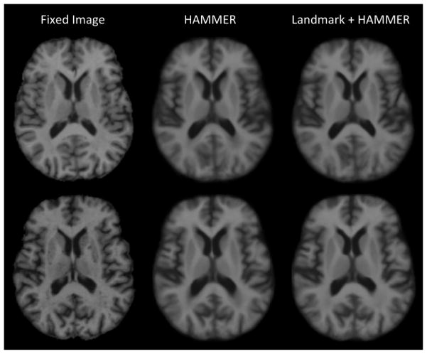
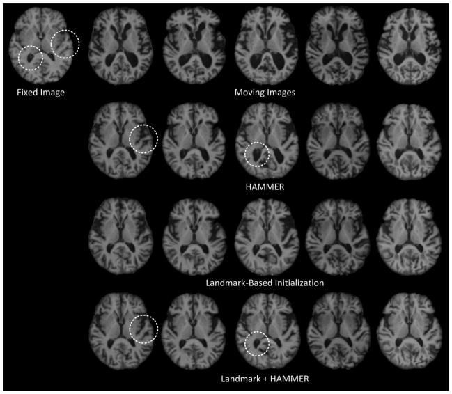
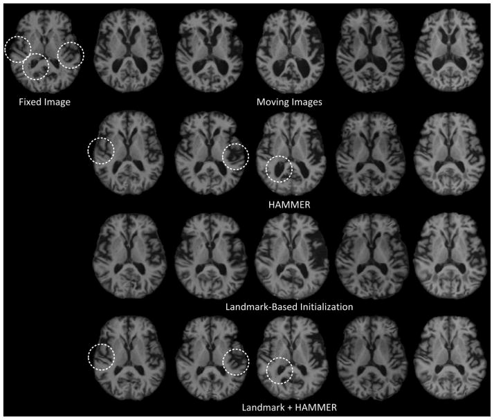
Fig. 10 shows the fixed images and the average images of all the warped images produced by HAMMER alone and Landmark+HAMMER, respectively, for both Case 1 and Case 2. Through visual inspection, the average images given by Landmark+HAMMER are sharper than those given by HAMMER alone, especially in the ventricular areas. To better illustrate the advantage of our approach, we select 5 images from the testing set that are substantially different in appearance from the fixed images in both Case 1 and Case 2. Figs. 11 and 12 present the registration results for Case 1 and Case 2, respectively. These two figures clearly demonstrate the registration improvements given by the Landmark+HAMMER. After landmark-based initialization, the inter-subject differences of these MR brain images are significantly reduced. Further improvements are obtained by refinement using HAMMER.

Fig. 10.

The fixed images and the corresponding average images of all the warped images produced by HAMMER alone and Landmark+HAMMER for both Case 1 (first row) and Case 2 (second row).

Fig. 11.

Registration results of 5 images that are substantially different from the fixed image in Case 1. The first row consists of the fixed image and the original moving images. The second row consists of the results from HAMMER alone. The third row consists of the results given by landmark-based initialization. The fourth row consists of the results given by refinement using HAMMER.

Fig. 12.

Registration results of 5 images that are substantially different from the fixed image in Case 2. The first row consists of the fixed image and the original moving images. The second row consists of the results from HAMMER alone. The third row consists of the results given by landmark-based initialization. The fourth row consists of the results given by refinement using HAMMER.

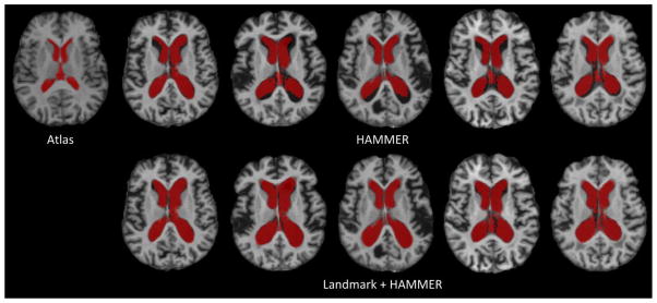
Next, we evaluated the registration performance of Landmark+HAMMER in labeling the ventricular regions in the testing images. Specifically, the fixed image in Fig. 11 was used as the atlas, and the ventricle label in the atlas was mapped to the 5 moving images in Fig. 11 by using the deformation fields estimated by image registration. Fig. 13 shows the results from HAMMER and Landmark+HAMMER, respectively. It is apparent that when the images are quite different from the atlas, Landmark+HAMMER can achieve better accuracy in ventricle labeling (see the red regions in Fig. 13).

Fig. 13.

The labeling results for the ventricular regions in 5 testing images. The fixed image in Fig. 11 was used as the atlas, and the ventricle label in the atlas was mapped to the 5 moving images in Fig. 11 by using the deformation fields estimated by image registration. Labeling results given by both HAMMER (first row) and Landmark+HAMMER (second row) are presented.

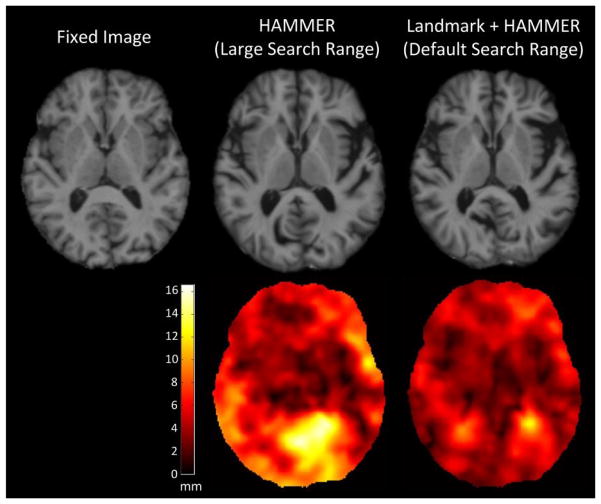
From the above experiments we can see that, when the moving image is substantially different from the fixed image, the large differences may not be handled well by using HAMMER alone. One possible solution to this problem is to use more aggressive parameters. For instance, we can use a larger search range. However, increasing the search range may introduce other issues, e.g., the risk of introducing false-positive correspondences. In addition, the deformation fields may be bumpy, indicating structural mapping that may not be biologically feasible. To better illustrate this point, we used HAMMER again, but with a larger search range, to warp the third moving image to the fixed image in Fig. 11. Then, the result given by HAMMER (with a larger search range) was compared with that given by Landmark+HAMMER (with default search range). From the results shown in Fig. 14, we can see that the ventricular region in the warped image from HAMMER is well aligned, but at the cost of less-accurate registration in the cortical regions. This can be better understood from the magnitude maps of the deformation fields estimated by the two methods. From these deformation magnitude maps, we can see that the deformation field generated by HAMMER is quite bumpy and the displacement values of some regions are unrealistically large. Landmark+HAMMER generates a smoother deformation field with largest displacements around the ventricular region, which seems to agree with the images. This experiment further demonstrates the advantage of Landmark+HAMMER.

Fig. 14.

Registration results given by HAMMER (with a larger search range) and Landmark+HAMMER (with default search range). The first row consists of the fixed image and the two warped images. The second row consists of the corresponding magnitude maps of the deformation fields. Greater brightness indicates larger magnitude of deformation.

3.3.2 18-Elderly-Brain dataset

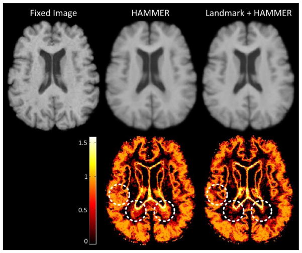
To further evaluate the robustness of the landmark-based initialization method, we also applied these learned landmark detectors to the 18-Elderly-Brain dataset. In this experiment, one image was selected as the fixed image, and the other 17 images were warped to it. Registration results from the Landmark+HAMMER approach and HAMMER alone were obtained. Table 4 presents the Dice ratios and the corresponding standard deviations of VN, GM and WM regions for both methods. From Table 4 we can see that, compared with the original HAMMER, the Landmark+HAMMER approach achieves higher Dice ratios and lower standard deviations for all tissue types, which is quite similar with the results on the ADNI dataset. To quantify the consistency of the registration results, we further calculate the entropy of tissue type probability across all warped segmentation images voxel by voxel. A lower entropy value at a voxel indicates higher registration consistency at this voxel. In this experiment, the average entropy values for HAMMER and Landmark+HAMMER are 0.44 and 0.42, respectively. Fig. 15 shows the average images of all warped moving images produced by HAMMER and Landmark+HAMMER, respectively, and the corresponding entropy maps of tissue type probability. Improvements in registration consistency by the Landmark+HAMMER approach can be easily observed in Fig. 15. This experiment well demonstrates the applicability of the landmark-based initialization method to different MR brain image datasets.

Table 4.

The Dice ratios and the corresponding standard deviations of VN, GM and WM regions, for both the Landmark+HAMMER approach and the original HAMMER.

Region	Before Reg.	Landmark+HAMMER	HAMMER
VN	64.7% (±9.39%)	84.1% (±2.67%)	81.9% (±5.43%)
GM	52.4% (±1.85%)	67.8% (±1.60%)	66.7% (±1.97%)
WM	61.7% (±2.62%)	76.1% (±1.39%)	74.6% (±1.85%)

Fig. 15.

This figure illustrates the registration performance of the original HAMMER and the Landmark+HAMMER approach on the 18-Elderly-Brain dataset. The first row shows the fixed image and the average images of all warped moving images produced by HAMMER and Landmark+HAMMER, respectively. The second row shows the corresponding entropy maps of tissue type probability for the two methods. Higher brightness indicates less registration consistency.

4. Conclusion

In this paper, we analyze the limitations of conventional anatomical correspondence detection methods, and then propose a multi-resolution regression-guided landmark detection method to overcome these limitations. In our method, regression forest is employed to learn the complex non-linear mapping from local image appearances to the 3D location of each landmark. The learned regression forest is utilized to detect latent corresponding landmarks in new images. Experimental results indicate that, when the structural differences of two images are significant, using HAMMER alone may not obtain satisfactory results. However, with the help of reliable correspondences obtained using the landmarks detected via the proposed method, structural differences between two subjects can be significantly reduced. Then, by refining the outcome using HAMMER, the final results are more accurate and robust than those given by HAMMER alone.

One limitation of the proposed method is that it uses only Haar-like features, i.e., intensity patch differences, to characterize a point in an image. Haar-like features are low-level features and are relatively sensitive to image contrast variations. Because MR brain images from different scanners can be different in contrast, the accuracy of landmark detection may be compromised. To alleviate this problem, histogram matching can be adopted in both training and application stages to normalize image contrast. Further improvements can be obtained by incorporating higher-level features, e.g., contrast-invariant features, into the proposed method. Future research will include (1) further improving landmark detection accuracy and (2) extending our regression forest framework to other potential application areas.

• We propose a novel method to detect distinctive landmarks for effective correspondence matching.

• Specifically, we use regression forest to simultaneously learn (1) the optimal sets of features to best characterize each landmark and (2) the non-linear mappings from the local patch appearances of image points to their 3D displacements towards each landmark. The learned regression forests are used as landmark detectors to predict the locations of these landmarks in new images.

• Because each detector is learned based on features that best distinguish the landmark from other points and also landmark detection is performed in the entire image domain, our method can address the limitations in conventional methods.

• Experimental results show that our method is capable of providing good initialization of registration, even for the images with large deformation difference, thus improving registration accuracy.

References

- Castillo E, Castillo R, Martinez J, Shenoy M, Guerrero T. Four-dimensional deformable image registration using trajectory modeling. Phys Med Biol. 2010;55:305–327. doi: 10.1088/0031-9155/55/1/018. [DOI] [PMC free article] [PubMed] [Google Scholar]
- Chen Y, An H, Zhu H, Stone T, Smith JK, Hall C, Bullitt E, Shen D, Lin W. White matter abnormalities revealed by diffusion tensor imaging in non-demented and demented HIV+ patients. Neuroimage. 2009;47:1154–1162. doi: 10.1016/j.neuroimage.2009.04.030. [DOI] [PMC free article] [PubMed] [Google Scholar]
- Criminisi A, Shotton J, Konukoglu E. Tech Rep MSR-TR-2011-114. Microsoft Research; 2011a. Decision forests for classification, regression, density estimation, manifold learning and semi-supervised learning. [Google Scholar]
- Criminisi A, Shotton J, Robertson D, Konukoglu E. Regression forests for efficient anatomy detection and localization in CT studies. MCV, MICCAI workshop; 2011b. [DOI] [PubMed] [Google Scholar]
- Fan Y, Rao H, Hurt H, Giannetta J, Korczykowski M, Shera D, Avants BB, Gee JC, Wang J, Shen D. Multivariate examination of brain abnormality using both structural and functional MRI. NeuroImage. 2007;36:1189–1199. doi: 10.1016/j.neuroimage.2007.04.009. [DOI] [PubMed] [Google Scholar]
- Jenkinson M, Smith SM. A global optimisation method for robust affine registration of brain images. Med Image Anal. 2001;5:143–156. doi: 10.1016/s1361-8415(01)00036-6. [DOI] [PubMed] [Google Scholar]
- Jenkinson M, Bannister PR, Brady JM, Smith SM. Improved optimisation for the robust and accurate linear registration and motion correction of brain images. NeuroImage. 2002;17:825–841. doi: 10.1016/s1053-8119(02)91132-8. [DOI] [PubMed] [Google Scholar]
- Lowe DG. Object recognition from local scale-invariant features. Proc of the International Conference on Computer Vision. 1999;2:1150–1157. [Google Scholar]
- Pauly O, Glocker B, Criminisi A, Mateus D, Martinez Moller A, Nekolla S, Navab N. Fast multiple organs detection and localization in whole-body MR Dixon sequences. MICCAI. 2011:239–247. doi: 10.1007/978-3-642-23626-6_30. [DOI] [PubMed] [Google Scholar]
- Shen D, Wong W, Ip HHS. Affine-invariant image retrieval by correspondence matching of shapes. Image Vision Comput. 1999;17:489–499. [Google Scholar]
- Shen D, Davatzikos C. HAMMER: hierarchical attribute matching mechanism for elastic registration. IEEE Trans Med Imaging. 2002;21:1421–1439. doi: 10.1109/TMI.2002.803111. [DOI] [PubMed] [Google Scholar]
- Shen D. Fast image registration by hierarchical soft correspondence detection. Pattern Recogn. 2009;42:954–961. doi: 10.1016/j.patcog.2008.08.032. [DOI] [PMC free article] [PubMed] [Google Scholar]
- Van Rijsbergen CJ. Information retrieval. 2. Butterworth-Heinemann; London: 1979. [Google Scholar]
- Wee CY, Yap PT, Li W, Denny K, Browndyke JN, Potter GG, Welsh-Bohmer KA, Wang L, Shen D. Enriched white matter connectivity networks for accurate identification of MCI patients. Neuroimage. 2011;54:1812–1822. doi: 10.1016/j.neuroimage.2010.10.026. [DOI] [PMC free article] [PubMed] [Google Scholar]
- Wu G, Qi F, Shen D. Learning-based deformable registration of MR brain images. IEEE Trans Med Imaging. 2006;25:1145–1157. doi: 10.1109/tmi.2006.879320. [DOI] [PubMed] [Google Scholar]
- Wu G, Yap PT, Kim M, Shen D. TPS-HAMMER: Improving HAMMER registration algorithm by soft correspondence matching and thin-plate splines based deformation interpolation. NeuroImage. 2010;49:2225–2233. doi: 10.1016/j.neuroimage.2009.10.065. [DOI] [PMC free article] [PubMed] [Google Scholar]
- Wu G, Kim M, Wang Q, Shen D. S-HAMMER: Hierarchical attribute-guided, symmetric diffeomorphic registration for MR brain images. Hum Brain Mapp. 2013 doi: 10.1002/hbm.22233. [DOI] [PMC free article] [PubMed] [Google Scholar]
- Xue Z, Shen D, Davatzikos C. Determining correspondence in 3-D MR brain images using attribute vectors as morphological signatures of voxels. IEEE Trans Med Imaging. 2004;23:1276–1291. doi: 10.1109/TMI.2004.834616. [DOI] [PubMed] [Google Scholar]
- Xue Z, Shen D, Karacali B, Stern J, Rottenberg D, Davatzikos C. Simulating deformations of MR brain images for validation of atlas-based segmentation and registration algorithms. NeuroImage. 2006;33:855–866. doi: 10.1016/j.neuroimage.2006.08.007. [DOI] [PMC free article] [PubMed] [Google Scholar]
- Yang J, Shen D, Davatzikos C, Verma R. Diffusion tensor image registration using tensor geometry and orientation features. Medical Image Computing and Computer-Assisted Intervention - MICCAI. 2008;2008:905–913. doi: 10.1007/978-3-540-85990-1_109. [DOI] [PubMed] [Google Scholar]
- Zacharaki EI, Shen D, Lee SK, Davatzikos SK. ORBIT: a multiresolution framework for deformable registration of brain tumor images. IEEE Trans Med Imaging. 2008;27:1003–1017. doi: 10.1109/TMI.2008.916954. [DOI] [PMC free article] [PubMed] [Google Scholar]
- Zacharaki EI, Hogea CS, Shen D, Biros G, Davatzikos C. Non-diffeomorphic registration of brain tumor images by simulating tissue loss and tumor growth. Neuroimage. 2009;46:762–774. doi: 10.1016/j.neuroimage.2009.01.051. [DOI] [PMC free article] [PubMed] [Google Scholar]
- Zhan Y, Feldman M, Tomaszeweski J, Davatzikos C, Shen D. Registering histological and MR images of prostate for image-based cancer detection. Medical Image Computing and Computer-Assisted Intervention - MICCAI. 2006;2006:620–628. doi: 10.1007/11866763_76. [DOI] [PubMed] [Google Scholar]
- Zhang Y, Brady M, Smith S. Segmentation of brain MR images through a hidden Markov random field model and the expectation-maximization algorithm. IEEE Trans Med Imaging. 2001;20:45–57. doi: 10.1109/42.906424. [DOI] [PubMed] [Google Scholar]
- Zhang D, Wang Y, Zhou L, Yuan H, Shen D. Multimodal classification of Alzheimer’s disease and mild cognitive impairment. Neuroimage. 2011;55:856–867. doi: 10.1016/j.neuroimage.2011.01.008. [DOI] [PMC free article] [PubMed] [Google Scholar]
- Donner R, Menze B, Bischof H, Langs G. Global localization of 3D anatomical structures by pre-filtered Hough forests and discrete optimization. Medical Image Analysis. 2013;17:1304–1314. doi: 10.1016/j.media.2013.02.004. [DOI] [PMC free article] [PubMed] [Google Scholar]
- Lindner C, Thiagarajah S, Wilkinson JM, Wallis G, Cootes T Consortium T. Fully automatic segmentation of the proximal femur using random forest regression voting. IEEE Transactions on Medical Imaging. 2013;32:1462–1472. doi: 10.1109/TMI.2013.2258030. [DOI] [PubMed] [Google Scholar]
- Han D, Gao Y, Wu G, Yap P, Shen D. Robust Anatomical Landmark Detection for MR Brain Image Registration. Medical Image Computing and Computer Assisted Interventions (MICCAI) 2014;17:186–193. doi: 10.1007/978-3-319-10404-1_24. [DOI] [PMC free article] [PubMed] [Google Scholar]