Numerical simulation of the environmental impact of hydraulic fracturing of tight/shale gas reservoirs on near-surface groundwater: Background, base cases, shallow reservoirs, short-term gas, and water transport

Abstract

Hydrocarbon production from unconventional resources and the use of reservoir stimulation techniques, such as hydraulic fracturing, has grown explosively over the last decade. However, concerns have arisen that reservoir stimulation creates significant environmental threats through the creation of permeable pathways connecting the stimulated reservoir with shallower freshwater aquifers, thus resulting in the contamination of potable groundwater by escaping hydrocarbons or other reservoir fluids. This study investigates, by numerical simulation, gas and water transport between a shallow tight-gas reservoir and a shallower overlying freshwater aquifer following hydraulic fracturing operations, if such a connecting pathway has been created. We focus on two general failure scenarios: (1) communication between the reservoir and aquifer via a connecting fracture or fault and (2) communication via a deteriorated, preexisting nearby well. We conclude that the key factors driving short-term transport of gas include high permeability for the connecting pathway and the overall volume of the connecting feature. Production from the reservoir is likely to mitigate release through reduction of available free gas and lowering of reservoir pressure, and not producing may increase the potential for release. We also find that hydrostatic tight-gas reservoirs are unlikely to act as a continuing source of migrating gas, as gas contained within the newly formed hydraulic fracture is the primary source for potential contamination. Such incidents of gas escape are likely to be limited in duration and scope for hydrostatic reservoirs. Reliable field and laboratory data must be acquired to constrain the factors and determine the likelihood of these outcomes.

Key Points:

• Short-term leakage fractured reservoirs requires high-permeability pathways

• Production strategy affects the likelihood and magnitude of gas release

• Gas release is likely short-term, without additional driving forces

Introduction

Context of This Study

Hydrocarbon production from unconventional resources with ultralow permeability (tight) reservoirs has experienced tremendous growth over the last few years. Tight-sand and shale gas reservoirs (hereafter referred to as TG reservoirs) are currently the main unconventional resources, upon which the bulk of production activity is currently concentrating [Warlick, ²⁰⁰⁶]. Production from such resources in the U.S. has skyrocketed from virtually nil at the beginning of 2000, to where unconventional gas production is forecast to increase to 64% of total U.S. gas production by 2020 [American Petroleum Institute (API), ²⁰¹⁴]. The advent of effective reservoir stimulation techniques such as hydraulic fracturing has significantly increased the ability to recover natural gas from these TG formations, resulting in a dramatic increase in the estimate of the U.S. gas reserves. Thus, gas production from shale and tight-sand reservoirs has proven remarkably successful in increasing substantially both gas production and reserves estimates in the U.S. In addition to its financial benefits, the development of technology to produce fossil fuels in previously inaccessible domestic geologic systems is considered a significant contributor to energy security.

The universal feature of all TG reservoirs is the unavoidable need for well and reservoir stimulation: the matrix permeability is extremely low (often at the nano-Darcy level) and, even with the presence of a system of natural fractures, it cannot support flow at anything approaching commercially viable rates without permeability enhancement. Stimulation technology has made economical gas and oil production from shales possible. Such treatment develops a new system of artificial fractures that increase the permeability of the system and increase the surface area over which reservoir fluids flow from the matrix to the permeable fractures, providing access to larger volume of the reservoir. Conventional stimulation techniques are usually variants of hydraulic fracturing (HF) in which the artificial fracture system is induced by the injection of water or of a water-based medium into the fractures and the matrix of the geologic medium.

The substantial increase in gas production (and the corresponding economic benefits) derived from stimulation has been accompanied by controversy. Some of the controversy and environmental concern revolves around potential undesirable effects of stimulation to the subsurface beyond the confines of the TG, hydrocarbon-bearing formation. Generally speaking, the concerns are that reservoir stimulation creates significant environmental threats through the creation of fast permeability pathways (e.g., via the fracturing of overlying formations, or failure of the cement in imperfectly completed wells) connecting the stimulated TG reservoir volume with shallower freshwater aquifers. This could potentially have adverse environmental consequences in the form of contamination of these potable groundwater resources by escaping hydrocarbons and other reservoir fluids that ascend through the subsurface. This potential problem has been the subject of recent studies, and several reviews have been published concerning the hydraulic fracturing process and the corresponding potential hazards [Jackson et al., ^2013a; King, ²⁰¹²; Brantley et al., ²⁰¹⁴; Vengosh et al., ²⁰¹⁴; Bachu and Valencia, ²⁰¹⁴; Davies et al., ²⁰¹⁴].

Objective of This Study

The objective of this study is to evaluate by means of numerical simulation the short-term (over a 2 year period) transport of contaminants (initially, gas) from a TG reservoir toward the shallower aquifer, and to analyze the implications, focusing on the possible contamination of a shallow aquifer and identifying the dominant/important parameters and the main transport mechanisms.

It is important to clarify what the present study is and is not. It is a parametric study using generalized representations of single-well, single-pathway tight and shale-gas systems to identify the processes and parameters that could lead to rapid gas transport from TG formations to groundwater resources, and begin quantify their relative importance and effect. It is not a formal risk assessment. It is not a detailed representation of a specific formation, reservoir and aquifer, or of a particular hydraulic fracturing scenario or technique. The multiplicity of geologies and geometries that may exist in such TG/aquifer systems, and the wide variety of conditions that may be encountered during hydraulic fracturing operations make it impossible to predict all possible outcomes. However, by identifying the processes that enhance or mitigate flow and transport out of TG reservoirs, and by examining a range of geological parameters and production techniques, the envelope of potential system behavior (and of possible hazards) can be better defined. This may then inform well design, fracturing operations, production strategies, monitoring studies, and the scope of future modeling work.

The present study is also part of a larger effort. These results cover shallow reservoirs and hydrostatic conditions, but necessarily, the effects of overpressure and deeper formations must also be examined (along with other parameters). Future publications will apply the simulation methods used here to those types of systems.

Background

Formation of Pathways and Transport of Gas in the Subsurface

In a recent progress report concerning ongoing EPA studies of the potential impacts of hydraulic fracturing on groundwater resources [U. S. Environmental Protection Agency, ²⁰¹²], the authors state clearly that data concerning out-of-formation fracture propagation and subsequent contamination is currently very limited, with few peer-reviewed studies in place. The issue of contamination of groundwater resources due to hydraulic fracturing operations and gas production primarily hinges on two considerations. First, contaminant migration requires a pathway, whether natural or induced. This could involve fracturing processes that connect the reservoir to preexisting pathways, creating the pathways themselves via hydraulic fracturing, creating pathways during the process of well drilling and casing, or connecting to preexisting pathways during well drilling and casing. Second, subsurface processes may drive flow and transport of gas, oil, and other fluids, including flow and transport through faults, fractures, or other pathways (whether artificial or preexisting). Both a pathway and driving forces for subsurface flow must exist to create a hazard.

The formation of pathways has been addressed in a series of recent papers on coupled flow, thermal, and geomechanical response of TG reservoirs, funded as part of the same overall project (discussed in section 3). A coupled flow-geomechanical simulator [Kim and Moridis, ^,] developed using the established TOUGH+ subsurface flow and transport simulator code base [Moridis and Freeman, ²⁰¹⁴] was used to model fracture development, and found that shear failure can limit the extent of fracture propagation. Later work using full 3-D domains suggests inherent limitations to the extent of fracture propagation, particularly in the presence of overlying confining formations [Kim et al., ²⁰¹⁴], and that the overpressure conferred by stimulation is transient. Other recent research has discussed possible pathway formation (including limitations to the extent of vertical fracture propagation) [Flewelling et al., ²⁰¹³; Fisher and Warpinski, ²⁰¹²; Davies et al., ²⁰¹²; Jackson et al., ^2013a], but it is clear that additional research is required to better quantify this hazard. However, fracturing that creates pathways to preexisting pathways, whether naturally formed (permeable fractures or faults) or artificial (abandoned, degraded, poorly constructed, or failing wells) cannot be discounted, nor can the possibility of human error in the construction and operation of wells be ignored.

If it is the case that pathways can be created, then two possible routes have been suggested as particularly likely to affect shale-gas production—transport through connecting fractures and faults (whether natural, created, or a combination) and transport through offset wells (possibly degraded or compromised) connected to the production zone via fractures [Jackson et al., ^2013a; Kissinger et al., ²⁰¹³]. While postglacial processes and bedrock fracturing may make gas-producing regions more susceptible to gas and fluid migration even without stimulative fracturing (e.g., the Marcellus basin in Pennsylvania), there is also the presence of thousands of wells that predate the modern fossil energy era. As noted by Vidic et al. [2013], in Pennsylvania, about 200,000 wells date from before the inception of formal record keeping, and the status of 100,000 wells is essentially unknown. The older or abandoned wells may be subject to eventual degradation, creating more permeable casings over time with permeability levels on the k = 10⁻¹⁵ m² to 10⁻¹³ m² range [Crow et al., ²⁰¹⁰; Gasda et al., ²⁰¹³; Watson and Bachu, ²⁰⁰⁹], but only after decades of exposure to subsurface geochemistry. Results suggest that such enhanced permeability is also more a function of degradation of casing-to-cement or cement-to-formation bonding, rather than permeability of the cement itself [Gasda et al., ²⁰¹³]. Potential pathway formation outside of the casing is also seen as a plausible (and perhaps most-likely) source of potential migration [Dusseault and Jackson, ²⁰¹⁴] due to incomplete cementing or cement shrinkage.

The core literature on the subject of subsurface migration of contaminants includes a few groups of competing and contentious studies, none of which provide hard evidence in support or against direct links between fracturing operations, production from shales, and groundwater contamination, but which suggest strong correlations [Révész et al., ²⁰¹⁰; Osborn et al., ²⁰¹¹; Jackson et al., 2013a; ^2013b; Warner et al., ²⁰¹²; Molofsky et al., ²⁰¹³]. A clear conceptual model that ties stimulation and TG production to a specific instance of methane contamination has yet to be elucidated, and as such we have established correlation but not causation. A literature review by Flewelling and Sharma [2014] makes a case that strong upward gradients (considered unlikely) are necessary, along with permeable pathways, to drive upward migration, and notes that overpressured formations (to provide such driving forces) would have to be bounded by low-permeability caps in order to remain overpressured. Engelder et al. [2014] also question the likelihood of rapid transport, noting that data suggest reservoir water saturations in the range of 13%–33%, i.e., below the irreducible water saturation for the shale. This suggests imbibition and capillary binding of injected water, restriction of brine migration, and the possible sequestration of fracturing fluids remaining in the formation. Preexisting (i.e., before HF operations) brine migration may also confuse attempts to monitor groundwater for HF-related contamination [Llewellyn, ²⁰¹⁴].

Earlier Modeling Studies

Although several mechanisms for transport through fractures and faults have been proposed, few conclusions can yet be made about the parametric space under which fluids (gas and/or contaminated water) release can occur. A study by Myers et al. [2012] attempted to model flow through artificially created pathways. Using MODFLOW simulation, the work determined that the pressure increases are localized, subside in a year or less, and that the pressure of the injection-stimulated systems could reequilibrate within a year or less. The Myers study operated under the assumption of the existence of out-of-formation fractures or connectivity to permeable faults, which, if present, could drive fluids or gas into overlying formations on decadal scales or more quickly. This modeling has been criticized for assuming fully saturated shales [Vidic, 2013], which may be inaccurate and bias the results [Engelder et al., ²⁰¹⁴] toward fluid releases.

A recent modeling study by Kissinger et al. [2013] performed porous-media simulation of fluid and gas migration through a previously characterized, fractured system. Although focused on a single set of geological models, the study highlights factors that may increase or decrease the risk of contamination. Fluid migration due to a 2 week fracturing-related overpressure is shown to drive fluid only a limited distance from the fractured reservoir, even when high-permeability pathways are assumed. Long-term tracer transport and transport of methane to overlying aquifers is shown to be a function of pathway porosity, permeability, and irreducible gas saturation, but only under the assumption of a continuous permeability pathway from the reservoir to the aquifer. Another recent paper by Gassiat et al. [2013] examined 2-D transport of contaminants and found that transport on thousand-year timescales may be possible under reasonable hydrologic conditions. However, this paper attempts to use a single-phase aqueous system to represent a shale system (Utica Shale) that is actually undersaturated, and thus ignores important capillary effects that would reduce the ability of the reservoir overpressure to drive aqueous flow. This work also serves to illustrate the importance of including multiphase flow (including capillarity and relative permeability effects) in modeling of gas or contaminant migration from shales.

It is obvious that additional research is required to better quantify this hazard [Jackson et al., ^2013a], with a focus on (a) establishing background values of various contaminants, (b) field experiments and monitoring, and (c) better modeling studies to elucidate possible transport mechanisms. The present study aims to address the last of these issues.

The U.S. Environmental Protection Agency (EPA) Study

Background, Impetus For, and Focus of the Study

This study was conducted by staff of Lawrence Berkeley National Laboratory (LBNL) as part of a wider investigation headed by the EPA’s Office of Research and Development. This is in response to the Fiscal Year 2010 Department of the Interior, Environment, and Related Agencies Appropriations Act (P.L. 111-88), which directed EPA to “… carry out a study on the relationship between hydraulic fracturing and drinking water, using a credible approach that relies on the best available science, as well as independent sources of information. The conferees expect the study to be conducted through a transparent, peer-reviewed process that will ensure the validity and accuracy of the data. The Agency shall consult with other Federal agencies as well as appropriate State and interstate regulatory agencies in carrying out the study, which should be prepared in accordance with the Agency’s quality assurance principles.”

Of the wide scope of the EPA study, the LBNL investigation first identified the possible failure scenarios that can lead to contamination of groundwater resources following hydraulic fracturing operations, and then focused on two issues: the geomechanics issue, and the contaminant transport issue. In the first, we sought to determine (a) if the various failure scenarios following hydraulic fracturing were physically possible, and, (b) if so, under what properties and conditions (flow, geomechanical, hydraulic fracturing operations), as well as (c) the envelope of possible solutions. The results of this geomechanical component of the LBNL studies are reported elsewhere [Kim and Moridis, ²⁰¹³, 2014; Rutqvist et al., ²⁰¹³], and will not be further discussed here.

In the present paper, we focus exclusively on the contaminant transport component of the LBNL studies. Here we do not address the likelihood of pathway formation—such assessments are clearly indispensable for a thorough evaluation of the problem, but are not yet possible because of lack of any statistical data. Thus, in the contaminant transport studies we considered pathways between the TG reservoir and a shallow aquifer a given and aimed to determine the extent of short-term contaminant transport covering the widest possible spectrum of system properties and conditions, and under realistic regimes of pressure in the TG reservoir and the aquifer corresponding to gas and water production, respectively.

EPA Failure Scenarios

We identified the following plausible failure scenarios for the upward migration of contaminants (including natural gas, salts, organic, and inorganic compounds used in hydraulic fracturing fluids, native radionuclides, etc.) following stimulation:

(1) Vertically extensive fracturing of the formations bounding the TG reservoir because of inadequate design or implementation of the stimulation operation, with the resulting fractures reaching groundwater resources, or even permeable formations that communicate with (generally) shallower water-bearing strata (Figure 1a).

Figure 1.

Failure scenarios 1 and 2.

(2) Sealed/dormant fractures and faults that can be activated by the hydro-fracturing operation, creating pathways for upward migration of hydrocarbons and other contaminants (Figure 1b).

(3) Induced fractures/faults that reach groundwater resources after intercepting conventional hydrocarbon reservoirs, which may create an additional source.

(4) Hydraulic fracturing creates fractures that intercept older, abandoned unplugged wells (or their vicinity) that had served conventional reservoirs (Figure 2a). This can be caused by lack of information about the location and installation specifics of the abandoned wells, or because of inadequate design or implementation of the stimulation operation resulting in excessively long fractures. These aging wells can intersect and communicate with freshwater aquifers, and inadequate or failing completions/cement can create pathways for contaminants to reach the potable groundwater resources.

Figure 2.

Failure scenarios 4 and 5.

(5) Failure of the well completion during stimulation because of inadequate/inappropriate design, installation and/or weak cement (Figure 2b). In this case, the well itself is the weak link, and it either includes open voids, or is fractured during the stimulation process, or both. Thus, improper cementing and well completion can result in continuous, high-permeability pathways connecting the TG reservoir with the shallow aquifer, through which contaminants can ascend toward the surface. Note that the overlying formations may or may not be fractured in this case.

As the number of possible subsurface configurations is infinite, we must choose representative scenarios for evaluation. Scenario 3, presents too many variables (e.g., the nature, depth, pressure, and composition of the intermediate reservoir) to generalize, and can be seen as a subset of scenarios 1 and 2. By combining scenarios 1 through 3 and scenarios 4 and 5, we have two general sets of contamination pathways: faults/fractures (wide planar pathways) and degraded wells (i.e., an annular or tubular pathway of limited radial extent). These two pathway examples will be simulated over a range of pathway physical parameters to assess mechanisms of gas and water transport.

EPA Objectives

The overall purpose of the EPA study is to elucidate the relationship, if any, between hydraulic fracturing and drinking water resources. More specifically, the EPA study was designed to assess the potential impacts of hydraulic fracturing on drinking water resources and to identify the driving factors that affect the severity and frequency of any impacts. The specific objective of this component of the LBNL study is to evaluate by means of numerical simulation the transport of contaminants (initially, gas) from a TG reservoir toward the shallower aquifer, and to analyze the implications. Thus, we seek to (a) determine the extent of contaminant migration from the TG reservoir and the possible intrusion into the shallower aquifer under a wide variety of conditions, properties and parameters (covering a wide spectrum of field possibilities), and (b) to identify the dominant/important parameters, as well as the main transport mechanisms.

System Description and the Numerical Study

The Numerical Simulator

We conducted the numerical studies using the TOUGH+RealGasH2O simulator [Moridis and Freeman, ²⁰¹⁴], a member of the TOUGH family of codes [Pruess et al., ¹⁹⁹⁹] developed by LBNL. This simulator (hereafter referred to as T+RGW) describes the nonisothermal two-phase flow of water and a real gas mixture in gas reservoirs, with a particular focus in TG reservoirs. The gas mixture is treated as either a single pseudocomponent having a fixed composition, or as a multicomponent system composed of up to 9 individual real gases. In addition to the standard capabilities of all members of the TOUGH+ family of codes (fully implicit, compositional simulators using both structured and unstructured grids), the capabilities of the code include: coupled flow and thermal effects in porous and/or fractured media, real gas behavior, inertial (Klinkenberg) effects, full microflow treatment (Knudsen diffusion and the Dusty-Gas Model [Webb and Pruess, ²⁰⁰³; Freeman et al., ²⁰¹¹] for multicomponent studies), Darcy and non-Darcy [Forchheimer, 1901; Barree and Conway, ²⁰⁰⁷] flow through high-permeability features, single and multicomponent gas sorption onto the grains of the porous media following several sorption isotherms, discrete and equivalent fracture representation, complex matrix-fracture relationships, porosity-permeability dependence on pressure changes, and an option for full coupling with geomechanical models. The T+RGW code allows the study of flow and transport of fluids and heat over a wide range of time frames and spatial scales not only in gas reservoirs, but also in problems of geologic storage of greenhouse gas mixtures, and of geothermal reservoirs with multicomponent condensable (H₂O and CH₄) and noncondensable gas mixtures. The simulations performed for this study involve 3 simultaneous equations per gridbock (element), corresponding to the two mass balance equations for H₂O and CH₄, plus the heat balance equation of the entire system (i.e., nonisothermal). We also use Langmuir sorption for CH₄ in the shale reservoir (see Table1 for parameters) and microflow physics within the tight shale medium. The reader should refer to Moridis and Freeman [2014] and Freeman et al. [2011] for information about simulator development and validation, and to the TOUGH+ manual [Moridis, ^,], copies of which are also available via the US EPA.

Table 1.

Parametric Variations^a

F-Cases (144 total)
Fracture/fault permeability kf	1 × 10−12 m2	1 × 10−11 m2	1 × 10−9 m2
TG reservoir permeability ks	1 × 10−21 m2	1 × 10−19 m2	1 × 10−18 m2
Aquifer permeability ka	3 × 10−13 m2	3 × 10−12 m2
Production Strategy	Shale Well	Water Well	Both Wells	None
Separation distance L	200 m	800 m
W-Cases (192 total)
Well cement permeability kw	1 × 10−18 m2	1 × 10−15 m2	1 × 10−12 m2	1 × 10−9 m2
TG reservoir permeability ks	1 × 10−21 m2	1 × 10−19 m2	1 × 10−18 m2
Aquifer permeability ka	3 × 10−13 m2	3 × 10−12 m2
Production Strategy	Shale Well	Water Well	Both Wells	None
Separation distance L	200 m	800 m

^aBase-case values in bold.

Simulation Cases: Description, Specifications, and Assumptions

In the current study we investigate the contaminant transport potential of systems with the general geometric configurations described in the failure scenarios 1–5 (see section 3.2). These involve a vertical well in the shallow aquifer, a horizontal production wells in the TG reservoir (the stimulation of which is achieved by hydraulic fracturing), and a connecting permeable feature that penetrates an impermeable overburden (which we define here as the formations between the TG reservoir and aquifer, whether consolidated caprock or unconsolidated units). We focus on a set of cases which, in addition to the general features, include specific (a) distances between the subdomains of the system under investigation, (b) types of the permeable feature connecting the TG reservoir to the shallow freshwater aquifer, (c) formation conditions and properties, and (d) gas and water-well production regimes. These parametric dimensions were chosen a priori, and serve as a starting point for a more comprehensive analysis. Thus, the base cases involve the following:

1. Two types of permeable connecting features through which contaminants can ascend from the TG reservoir toward the aquifer. The first type is fractures or permeable faults that can be either entirely hydraulically induced (a possibility if the separation between the TG reservoir and the aquifer is limited), or comprising a lower hydraulically induced part emanating from the TG horizontal well and connecting to an upper section that can be a dormant (initially dead-end) natural fracture or a permeable fault. Such systems can represent failure scenarios 3–5 that are described in section 2.2 (the numerical representations of which are similar), and the corresponding cases are identified as F-cases. The system behavior is investigated for the following fracture permeabilities: k_f1 = 10⁻⁹ m², k_f2 = 10⁻¹¹ m², k_f3 = 10⁻¹² m² (1000 D, 10 D, and 1 D, respectively, where 1 D = 1 Darcy). The connecting fracture is assumed to be a vertical extension of the induced fracture in the TG domain in all F cases, to capture the connectivity of both a fracture that continues through the overburden, or a hydraulic fracture that intersects a preexisting planar pathway such as a natural fracture or fault.

   The second type is failed wells, and involves either hydraulically induced fractures that emanate from the TG reservoir and intercept older offset wells (serving conventional reservoirs and usually abandoned) with deteriorated casings, cement and even (possibly) tubing, or hydraulic fractures that are confined within the horizontal and vertical parts of the TG well. The latter can be caused by imperfections in the design and execution of the well installation and stimulation, which can result in weak cement (that can allow fracture creation and propagation during stimulation), continuous voids over large distances (if the cement is not in contact with the media), or both. Such systems can represent the failure scenarios 1 and 2 described in section 3.2 (the numerical representations of which are similar), and the corresponding cases are identified as W-cases. The system behavior was investigated for the following cement permeabilities: k_w1 = 10⁻⁹ m², k_w2 = 10⁻¹² m², k_w3 = 10⁻¹⁵ m² and k_w3 = 10⁻¹⁸ m² (1000 D, 1 D, 1 mD, and 1 µD, respectively). The distance between the horizontal gas production well and the offset (or the vertical part of the horizontal) well was assumed to be D_w = 10 m in all W-cases (i.e., the offset well is directly connected to the fracture in the TG reservoir). This allows us to approximate, in this early study, both degradation of the vertical casing of the horizontal gas production well and connectivity with a nearby abandoned and degraded well. Note that connecting fractures have larger total volumes per unit length than annular pathways around failed wells, as the fracture has a larger y dimension than the circumference of a near-well annular region.

2. Two separation distances L between the TG reservoir and the aquifer: L₁ = 200 m and L₂ = 800 m. A third separation distance of L₃ = 2000 m is investigated in a continuing study (to be reported in a forthcoming companion paper), and is limited only to cases that indicate probability of measurable contamination when L₂ = 800 m. While the value of L₁ = 200 m may be an unlikely geometry, it is important to capture an end-case where contaminant transport is highly likely to contrast the result with more likely scenarios (i.e., larger separations).

3. Two aquifer permeability k_a values: k_a1 = 10⁻¹² m² and k_a2 = 10⁻¹³ m² (1 D and 0.1 D, respectively).

4. Three TG reservoir matrix permeability k_s values: k_s1 = 10⁻¹⁸ m², k_s2 = 10⁻¹⁹ m² and k_s3 = 10⁻²¹ m² (1 µD, 100 nD, and 1 nD, respectively), which give a parametric range from microdarcy (the most permeable shales) to nanodarcy conditions [Neuzil, ¹⁹⁹⁴; Hill and Nelson, ²⁰⁰⁰].

5. Four water and gas production regimes: (a) both the gas well and the water well are producing, (b) only the water well is producing (inactive gas well), (c) only the gas well is producing (inactive water well), and (d) no water or gas production (both the water and the gas well are inactive).

6. A hydrostatic initial pressure distribution in the aquifer, TG reservoir, and any pathway. Overpressured reservoirs will be addressed in a subsequent paper.

A listing of the parameters varied as part of the parametric study, and their values, are listed in Table1. In all the base cases the aquifer and the TG reservoir are assumed to be infinite acting. When gas is produced, the horizontal well is operated at a constant bottomhole pressure P_w = 0.5 P₀, i.e., at half the discovery (initial) pressure of the TG reservoir. When water is produced, it is withdrawn from the aquifer via the vertical well at a constant mass flow rate of Q_w = 0.1 kg/s (8.64 m³/d). The relative permeability and capillary pressure functions and parameters of the sandy aquifer and of the TG formation are different from each other, but they are the same in all base cases. The common (to all simulations) system conditions, properties, and relevant parameters are listed in Table2.

Table 2.

Common Simulation Parameters

Aquifer temperature (top)	12°C
Aquifer pressure (top)	1.0 MPa
Reservoir temperature (depth dependent)	21–24°C, 39–42°C
Reservoir pressure (depth dependent, hydrostatic)	4.44 MPa, 10.3 MPa
Geothermal gradient dT/dz	0.03°C/m
Grain density ρR (all formations)	2600 kg/m3
TG reservoir porosity ϕs	0.05
Aquifer porosity ϕa	0.25
Well cement porosity ϕw	0.05
Fracture porosity ϕf	0.80
Composite thermal conductivity model [Sommerton, 1974]	kQC = kQRD + (kQRW – kQRD)
Dry thermal conductivity kQRD (TG reservoir and overburden)	1.5 W/m/K
Dry thermal conductivity kQRD (aquifer)	0.5 W/m/K
Wet thermal conductivity kQRW (TG reservoir and overburden)	4.0 W/m/K
Wet thermal conductivity kQRW (aquifer)	3.1 W/m/K
Capillary pressure model [van Genuchten, 1980]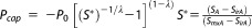
λ(all formations)	0.77
P0 (shales) [Sigal, 2013]	1.25 × 105 Pa
P0 (aquifer)	5.0 × 103 Pa
Relative permeability model	krA = (SA*)n
	SA* = (SA-SirA)/(1-SirA)
	SG* = (SG-SirG)/(1-SirA)
SirA (TG reservoir)	0.75
SirA (aquifer)	0.2
SirG (TG reservoir)	0.05
SirG (aquifer)	0.01
Water well production rate (if present)	0.1 kg/s
Gas well Pw (if present)	½ Ps0
Gas sorption isotherm: Langmuir (shales only)	S = As P/(Bs + P) (kg gas/kg solids)
	As = 7 × 10−3 Pa−1
	Bs = 107 Pa

The maximum time frame of the simulations in the first stage of this study is a relatively short 2 years, and was determined through initial scoping calculations that suggested a possible short-term nature of the gas release and predicted significant early flows in the majority of the base cases. Thus, we are testing the hypothesis that rapid escape of detectable quantities of gas may occur soon after the hydraulic fracturing process and during early production phases. Many simulations in fact reach a quasi-steady state well before 2 years, and thus stop for lack of significant changes in system properties. Selected simulations (i.e., parametric combinations) that exhibit significant fluid flow but show no gas breakthrough into the aquifer or at the water well within 2 years (or show no approach to steady state or equilibrium conditions) will be investigated for longer periods, and these results will be discussed in a subsequent paper.

Of the various possible contaminants (natural gas, native salts, chemical compounds used in hydraulic fracturing fluids, etc.), in the present paper we focus on natural gas, which we represent in the simulations as 100% CH₄. Additionally, we seek to determine if there is a dominant direction of water flow or a predictable water flow pattern, as this information can guide the direction of further investigations, particularly those that will include other dissolved species in the formation water.

Because it is not possible to study every possible combination of geological and well operation conditions, properties, and parameters, in this study we chose to examine the ones, in our judgment, we think are the most relevant and important. As knowledge is gained with this study, future simulation work can explore additional areas of parametric space that seem promising.

The 3-D Mesh

The TOUGH+ simulations for this study were run on three-dimensional Voronoi grids with geometric features informed by the geology of interest. We used the MeshVoro toolkit for generating these grids [Freeman et al., ²⁰¹⁴]. Because of the critical importance of representative 3-D grids in analyzing the problem under investigation, we discuss the mesh generation process in detail.

In addition to the geometries of the aquifer and of the TG reservoir, there are two families of geometries that correspond to the two general types of the permeable/connecting pathways in the base cases of our study. In the F-cases, we describe a subdomain containing the planar fracture that represents a hydraulic fracture (or a hydraulic fracture intercepting a native fracture or permeable fault) connecting the deeper TG reservoir to the shallow aquifer. This is designated as the F-family of grids. In the W-cases, we use a more complex geometry that includes (a) a cylindrical subdomain (which describes an abandoned well that descends below the aquifer into the TG reservoir overburden) intercepting (b) a planar subdomain that represents the hydraulic fracture emanating from the horizontal well in the TG reservoir. This is designated as the W-family of grids. The process of generating the 3-D grids for each family is generally the same, and is as follows:

1. We generate a set of points using a code that constructs point representations of geometric primitives such as boxes, planes, and cylinders. These points correspond to Voronoi generators, which correspond to cells in the final grid [Freeman et al., ²⁰¹⁴]. The process of generating these points involves overlaying the various geometric objects in space, and subsequent removal of any duplicate points introduced in the overlay.

2. The points are marked with labels that are used to associate various attributes, such as material properties and/or initial conditions or boundary conditions. This step is performed in the same code as in step 1.

3. The Voronoi tesselator feature of the MeshVoro application uses the field of points to generate a three-dimensional Voronoi mesh. It is possible to smooth the grid by using the Lloyd iteration process [Lloyd, ¹⁹⁸²] to improve the isotropy of the Voronoi cells, but we did not use this approach because it can lead to an erosion of the quality of the geometric representation.

One unfortunate limitation of the MeshVoro software (a Fortran/C-based toolkit, not a stand-alone application or a GUI-based tool) and the TOUGH-family mesh format [Moridis, ^2014a] is that we generate volume meshes, not finite-element meshes, and such volume meshes are not easily visualized (information about edges and faces of elements is not generated, nor does TOUGH+ require it) at this large scale with off-the-shelf tools. Visualizing arbitrary polyhedra, i.e., elements of an unstructured or nonregular mesh, is an area of active research [Freeman et al., ²⁰¹⁴], and the scope of this project could not accommodate development of such stand-alone tools.

Dimensions of the System Subdomains

The dimensions of the F and W-cases can be seen in a general form in Figure 3. The geometric parameters used in the mesh generation process are listed in Table3.

Figure 3.

General schematic and dimensions of the (a) F-cases and (b) W-cases.

Table 3.

Geometric Parameters

Aquifer – TG reservoir separation L	200 m, 800 m (see Table1)
Aquifer thickness ZA	100 m
TG Reservoir Thickness ZTG	100 m
Aquifer length, width ΔXA, ΔYA	1000 m
TG Reservoir (stencil) length ΔX	100 m
TG Reservoir (stencil) width ΔY	300 m
Distance from fracture plane to water well Dw	100 m
Hydraulic fracture height ΔZfTG	100 m (= ΔZΤΓ)
Hydraulic fracture width ΔYfTG	300 m (= ΔYΤΓ)
Hydraulic fracture aperture	1 mm
Penetrating fracture length (if present)	200 m + L
Penetrating fracture width (if present)	20 m
Penetrating offset well length (if present)	200 m + L
Penetrating well offset ΔYhv (if present)	10 m

The TG reservoir subdomain and the aquifer subdomain have the same dimensions in both the F and W-family geometries. Thus, the thickness of the aquifer and of the TG reservoir are ΔZ_A = 100 m and ΔZ_TG = 100 m, respectively. The aquifer extends in the x and y directions to ΔX_A = ΔY_A = 1000 m, with the fracture plane being at its center (Figures 3a and 3b). These dimensions, confirmed by scoping numerical simulation studies and coupled with constant-P boundaries (hydrostatic values) at its perimeter, ensured infinite-acting behavior of the aquifer during water withdrawal throughout the simulation period. Because of the much lower permeability of the TG reservoir, infinite-acting behavior over the 2 years of the study could be ensured by ΔX_TG =100 m and ΔY_TG = 300 m. Elements near the boundaries of the TG reservoir (away from the fracture and well) are monitored to ensure no pressure or temperature changes propagate to these boundaries during the simulation timeframe.

The hydraulically induced fracture within the TG reservoir has dimensions of ΔZ_fTG = 100 m (the reservoir thickness) and ΔY_fTG = 300 m, with the horizontal well being at the center of the rectangle (Figures 3a and 3b). The real fracture aperture was 1 mm, but was geometrically represented in the grid by a 1 cm wide element (necessitated by the demands of the MeshVoro application) and by a corresponding adjustment in porosity to ensure the correct fracture volume. We confirmed the numerical equivalence of the two systems by a simple numerical test, which yielded nearly identical results.

The fractures through the overlying formations (either hydraulic or natural) in the F-cases are assumed to have an average width of ΔY_fO = 20 m and the same aperture as the fractures within the TG reservoir (Figure 3a). The radius of the degraded region around the offset well (or the vertical part of the gas well) in the W-cases is meshed to approximately 0.5 m with a small porosity reflecting voids or deterioration in the region surrounding the well. With these dimensions, the pore volume of the connecting pathway in the W-cases is about one fifth of that in the F-cases.

The grid generation system, like other software developed in conjunction with this study, has been designed to cover a large parametric space. For this base study, we selected aquifer—TG reservoir separation as the geometric parameter to vary, while retaining the ability within the meshing tools to change other geometric parameters in future investigations (particularly after the base study provides information about what may or may not be important).

The F-Family of Grids

The fracture runs along the y axis. The F-family (Figure 3a) is defined by three parameters:

(1) The vertical separation (L₁ = 200 m or L₂ = 800 m) between the bottom of the aquifer and the top of the TG layer.

(2) The width ΔY_fO = 20 m of the connecting fracture along the y axis.

(3) The distance D_w = 100 m of the fracture from the water well in the aquifer.

For the base investigations of the F-cases, the total number of F-cases for the L₁ separation is N_FL1 = 72, and for L₂ separation is N_FL2 = 72. This system has bilateral symmetry with the bisection plane at y = 0, and the water well within the aquifer and the shale gas well lie on the axis of symmetry. Thus, we simulate half of the system described, and double the water and gas flow values.

The W-Family of Grids

Unlike the grids in the F-family, this system has no symmetry, and therefore must be simulated as a full 3-D system. The connecting well (between the TG reservoir and the aquifer) is offset (see Figure 3b) and is assumed to represent an abandoned well connecting to a deeper formation. The W-family has 6 parameters that determine the specific geometry of each case:

a. The vertical separation between the bottom of the aquifer and the top of the TG layer.

b. A vertical offset ΔZ_fO from the bottom of the connecting well to the top of the TG layer. This is also the height of the planar fracture below the well.

c. The distance D_w of the fracture (and in this case, the plane intersected by the offset well) from the water well in the aquifer.

d. The distance ΔY_hv along the y axis between the gas well in the TG and the offset well.

e. The width ΔY_fO of the fracture along the y axis beneath the connecting well.

For the base investigations of the W-cases, (a) L₁ = 200 m or L₂ = 800 m, (b) ΔZ_fO = 0 m (well penetrates the entire TG zone), (c) D_w = 100 m, (d) ΔY_hv = 10 m (the TG well intersects the fracture), while (e) is not applicable here because offset well fully penetrates the shale. The total number of W-cases for the L₁ separation is N_WL1 = 96, and for L₂ separation is N_WL2 = 96.

A summary of the common geometric parameters for all cases is also provided in Table3.

The Grid Generation Process

In each family of grids, we define a background layer of points on a cubic lattice at a variable resolution in the domain of interest. We then overlay a rectangular lattice of points at variable resolutions in the TG reservoir, the overburden and the aquifer (as high as 0.05 in the vicinity of the walls of the hydraulic fractures and around the offset well in the W-cases), removing any coincident points. To smooth transitions between high and low-resolution regions, we use logarithmic progressions in the x and y directions, maintaining regular gridding wherever possible to minimize mesh complexity. These generation parameters are manipulated by-hand within the MeshVoro scripting toolkit.

To represent a well in the W-family of grids, we clear all points within a rectangular box surrounding the well region and then generate a set of cylindrically arranged points around the well axis. Thus, a well has a single point at its center and a number of concentric layers of radial cells. At a given elevation, the subdivisions along the radial direction are logarithmically distributed, with radial intervals Δr_i = 1.2 Δr_i-1.

To minimize the number of points needed to accurately represent the vertical well in the W-cases, and to improve the isotropy of the radial cells within, we constrain the arc length of each cell to be approximately equal to its radial extent. This procedure produces irregularities in the angular distribution of the well cells, so that the resulting point distribution looks more like a bundle of fibers than a set of concentric regular polygons. However, we have determined that the well representation as a “fiber bundle” produces satisfactory results without needing large numbers of points (considering that we are simulating a degraded zone around the well, rather than discrete features like nested casings).

The hydraulically induced fracture in the F and W-families of grids is represented by a pair of planes of points on a square lattice with a 1 m resolution in z direction, and discretization matching that of the shale or neighboring overburden in the y direction. The fracture lies in the middle of the two planes, which are separated by an “apparent” fracture aperture of 1 cm, corresponding to a nominal fracture aperture. Note, however, that the behavior of the true fracture geometry is ensured by using the appropriate permeability k_f and by adjusting the fracture porosity to reflect the true fracture volume corresponding to an aperture of 1 mm. The use of the apparent fracture aperture is necessitated by both gridding difficulties of the Voronoi meshes and by numerical considerations stemming from such a discretization. Because of the way that Voronoi meshes are created, it is impossible to directly impose communication between any pair of cells—one must place the cells close enough together so that they are "visible" to one another. Accordingly, some care is required to ensure sufficient resolution at the intersections of geometric objects, such as a well and a fracture.

It is important to note that the generation of complex meshes such as those used here is not an automated process. Each generated mesh has to be evaluated for correctness and numerical tractability. This is accomplished at two points in the setup process. First, both the generating points and resulting mesh centroids and volumes must be carefully checked and confirmed for each configuration. Second, during gravity equilibration (i.e., when the initial pressure distribution is determined), the behavior of the system is monitored to ensure that stable hydrostatic and thermal equilibrium can be reached quickly without numerical reflections or oscillations. Third, each mesh configuration is tested interactively under a base-case simulation condition to evaluate the two-phase flow behavior in the TG reservoir and within the connecting feature. In this manner it is possible to identify problems associated with excessively fine or excessively coarse discretization, as well as other problems related to mesh connectivity, before batch simulations are attempted. Additional test simulations were used to explore beyond the core set of parameters, particularly to seek out important physical processes that may have been neglected due to the initial discretization. For example, such tests revealed the importance of selective refinement of areas around the fracture to capture leak-off or imbibition behavior.

The mesh generation process listed resulted in meshes with as few as 75,000 elements and 250,000 connections (planar fracture, 200 m separation) to as many as 245,000 elements and 881,000 connections (offset well, 800 m separation). These simulated systems are at the upper limit of fully implicit simulation on a typical modern desktop computer.

Conditions, Properties and Initialization

All the simulations were conducted nonisothermally, and the initial temperature followed the standard geothermal distribution with a midrange geothermal gradient of dT/dz = 0.03°C/m [SLB, ²⁰¹⁴], with T_tA = 12°C at the top of the aquifer. For the L₁ = 200 m and L₂ = 800 m overburden thickness, this results in T_tTG = 21°C or T_tTG = 40°C at the top of the TG reservoir. Deeper, hotter formations (for larger overburden thicknesses) will be discussed in the subsequent paper. The significant temperature difference between the gas reservoir and the aquifer, and the strong dependence of gas density on both P and T, did not permit treating the problem as isothermal.

We achieved initial thermal and pressure equilibration by maintaining constant boundary conditions and running a long-term simulation to a steady state by assuming highly permeable formations (the level of permeability is unimportant for the initialization process) and fully water-saturated initial conditions in the entire system profile. After reaching hydrostatic equilibrium, the intermediate layer was made impermeable, the system was brought to thermal equilibrium, then gas at the S_G = 0.7 level was introduced into the TG reservoir. Then the impermeable regions of the intermediate layer were removed, and the simulation was prepared for production simulations.

The aquifer and the overburden of the TG formation (including any connecting pathway) were fully water-saturated. The aqueous and gas saturations in the matrix of the TG reservoir were set at S_A = 0.3 and S_G = 0.7 respectively (highly undersaturated), which is consistent with earlier studies [Engelder, 2014] showing that many gas shales do not produce significant aqueous phase after flowback. The relative permeability and capillary pressure equations, as well as the relevant parameters, appear in Table2, along with all relevant reservoir properties.

The high-permeability pathways (F and W-features) were initially water-filled for pressure and temperature equilibration. For the production simulations, the hydraulic fractures within the TG reservoir are represented as gas-filled. The latter condition maximizes the volume of gas available for migration toward the aquifer, but it reflects a realistic scenario: although two-phase conditions are certain to occur within the hydraulic fractures during the hydraulic fracturing process and its aftermath, the removal of the fracturing fluids (referred to as the flowback or return water) prior to the initiation of production is almost certain to remove much of the water from the fractures. Since we cannot select a single initial water saturation that is reflective of all postfracturing conditions, we select the simplest initial state. However, the total gas volume in the hydraulic fracture is still low in absolute terms because of the limited fracture volume.

Other Important Assumptions

Other important assumptions are as follows:

1. The permeable connecting pathways (penetrating fractures and well casings) have uniform porosities and permeabilities throughout their entire length, including the 100 m zones of penetration through the TG reservoir and the aquifer. Partial penetration cases may be explored in future simulations.

2. The penetrating feature (well or fracture/fault) is the only permeable connection between the TG reservoir and the aquifer. The overburden is considered entirely impermeable. The meshing approximation is discussed in section 4.6. Transport through permeable overburdens has been explored in other studies [Gassiat et al., ²⁰¹³] (although only single-phase flow) and is expected to occur on multicentury timescales, not days, months, or years [Gassiat et al., ²⁰¹³; Flewelling and Sharma, ²⁰¹⁴]. Also, while permeable formation penetrated by the connecting feature could indeed absorb or divert migrating fluids, the infinite number of configurations of such additional permeable features are impossible to address in a parametric simulation study.

3. The numerical description of the offset wells in the W-cases implies transport through the fractures of the deteriorating cement between the subsurface formations and the outermost casing/conductor, through voids in the same region because of incomplete cement coverage of that space, or through breached tubing. This approach also covers the case of older, simple well installations without multiple casings. In the case of k_w = 10⁻⁹ m², this high-permeability represents, essentially, an open hole, which could mean either a breached tubing or incomplete cementing that left a continuous void that reaches the aquifer.

4. As already indicated, the aquifer treated as infinite, i.e., its outer boundaries are located at sufficiently large distances from the water to well and maintained at constant pressure, temperature, and composition (i.e., background level of dissolved CH₄, which represents a mass fraction X_A = 10⁻⁶ kg/kg or 0.1 mg/L).

5. The gas-bearing formation of the TG reservoir is initially undersaturated in water, with initial S_A0 = 0.3 (much lower than the irreducible S_Airr = 0.75). No leak-off (from stimulation) is considered through the fracture walls, which also have initial S_A0 = 0.3. By not assuming a larger initial S_A near the fracture walls, the permeability to gas (which is a very strong function of S_A) is not reduced, thus allowing easy flow into the open fracture (if driving forces exist) and providing a conservative scenario of unimpeded gas release. However, during the course of the simulation, imbibition of water into the undersaturated shale may occur given favorable capillary pressure regimes and invasion of water into the fracture. Variations in capillarity will be investigated in future publications, as well as simulation of the injection and leak-off processes.

6. Gas sorption (in the case of a shale gas reservoir) follows the Langmuir sorption isotherm [Freeman et al., ²⁰¹³]. The parameters and sorption equation are provided in Table2.

7. Only a 100 m-long segment of the TG well is represented, intercepted by the vertical hydraulic fracture at the midpoint; this is a valid approximation, as confirmed by the work of Olorode et al. [2013] and Freeman et al. [2013], who found that such reduced stencils are capable of accurately representing such systems over time frames exceeding hundreds of years. We assume one such fracture is connected to the communicating feature.

8. As indicated earlier, the study of the F-cases presupposes the existence of a continuous connecting permeable feature (natural fractures or permeable faults tied to hydraulically induced fractures), without considering the probability or possibility of such occurrences. This is an important assumption because the existence of such features cannot be ascertained. Formation of pathways has been discussed in earlier papers associated with this study [Kim and Moridis, ²⁰¹³; Rutqvist et al., ²⁰¹³; Kim and Moridis, ^{2013, 2014}].

9. In the W-cases, the connecting offset well is considered sealed at the top of the aquifer, i.e., transport via the offset well to formations above the aquifer is not considered.

Mesh Reduction Process

Because hundreds of individual simulations are required to explore the basic parametric space, reducing the meshes to the simplest useable configuration was crucial. One particular area of simplification is the treatment of the overburden through which the fracture or well ascends toward the aquifer. An impermeable overburden with full heat transfer treatment consumes a large portion of the total computational resources needed to perform a run. If this large region of largely unchanging elements can be reduced or removed, significant gains in efficiency (in terms of storage and execution speed) are possible.

After initial equilibration of the scenarios in the various base cases and the determination of the corresponding initial conditions, we simulated each scenario using the complete mesh, i.e., including the fully discretized overburden. We then reran the scenarios without the impermeable overburden (i.e., by removing the elements corresponding to the impermeable zone between the shale layer and the aquifer), and leaving only the connecting feature in place. Simulations performed with and without the overburden showed nearly identical results. This is not surprising, given that heat transfer from the mobile aqueous phase would have the greatest effect on gas temperature and therefore gas density, particularly when aqueous saturations are large. Removal of the impermeable zones results in computational speed gains nearly on par with isothermal simulation (corresponding to the reduction of the number of equations per gridblock by one), yet still allows the migrating aqueous and gas phases to correctly exchange heat in case where colder aquifer or pathway water interacts with warmer shale-originating gas or reservoir water.

Solution Monitoring

For each run, we monitor fluid flow (water and gas) through two interfaces. Interface #1 is at the plane at the top of the shale reservoir, and there we record the flow rates and the cumulative masses and volumes of water and gas in or out of the reservoir. Interface #2 is at the bottom of the aquifer, and there we monitor the flow rates and the cumulative masses and volumes of water and gas in or out of the aquifer. This allows tracking water and gas migration, i.e., whether they leave the TG reservoir and enter the connecting feature, and whether they leave the connecting feature and enters the aquifer.

In the cases of producing water or gas wells, we monitor the flow rates and the cumulative mass and volume of the aqueous and gas phases, as well as of CH₄, in addition to the gas-to-water ratio R_GW of the their mass flow rates in the production stream, and the mass fraction X_CH4 of the dissolved CH₄ in the water at the water well.

Simulation Management

For the exploration of the parametric space in the reference cases, the combination of the varying shale, pathway, and aquifer permeabilities, the two separation distances, and the four production strategies results in N_T = N_FL1 + N_FL2 + N_WL1 + N_WL2 = 336 unique sets of parameters for the base study, and thus 336 independent transport simulations. Additionally, we conducted well over 1,000 additional long and short-term simulations to clarify problems, confirm specific observations, or test the validity of the underlying assumptions. The large number of the T+RGW simulations necessitated the development of a new set of tools to allow batch submission and monitoring on the cluster used for the purpose. The approach involved the creation of a base “template” for the input files that identifies the connecting feature, separation, and production strategy, each combination of which requires its own initialization process. The batch software creates a series of labeled directories for each combination of parameters, copies the appropriate input files into each directory, sets the parameters within the main input file, and submits a job to the cluster queue to initiate a T+RGW run. As jobs stop or finish, the software can submit additional jobs as processors become available. This makes possible job submission to occur around the clock, allowing the efficient completion of the large number of simulations to be completed. It should be noted that the T+RGW simulations in this study can last from as little as a few days to as long as several weeks, and this automated process allows optimal use of computing resources. The automated system keeps track of the evolution of all the relevant parameters monitored in this study.

Early in the simulation process, it became apparent that progress was extremely slow in cases of extremely high permeability of the connecting feature (orders of magnitude slower than lower permeability cases). This was caused by the numerical challenge of resolving very small horizontal pressure gradients within the connecting feature after a very short initial period of rapid movement of gas and water. The simulations were made tractable by eliminating the horizontal connections (i.e., the horizontal flow) within the connecting features, an approach which we validated in a number of confirmatory tests that showed no perceptible impact on the results. The elimination of the horizontal connections resulted in a tenfold increase in time step size, with a commensurate decrease in the execution time.

Results and Discussion

The large number of flow and transport simulations in the base cases (N_T = 336) precludes the possibility of plotting all individual results. Thus, for each connecting feature (i.e., F and W-cases), we select only cases that elucidate interesting mechanisms or important concepts for more detailed presentation and discussion, and then present the overall parametric results by means of statistics—i.e., by plotting incidents of gas migration versus the various chosen parameters.

F-Base Cases: Transport Through Fractures and Faults

CH₄ Release, Transport and Production: L = L₁ = 200 m

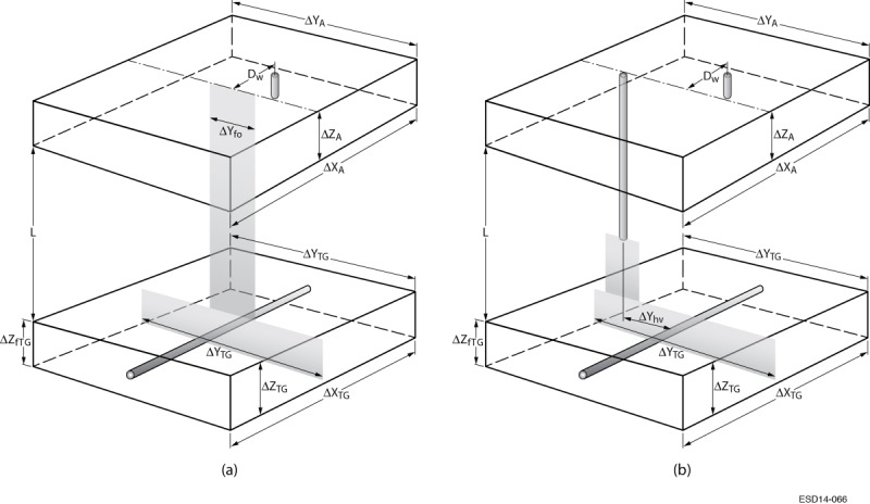
Figure 4 shows the volumetric flow rates of the free gas phase (practically 100% CH₄, with traces of H₂O vapor) leaving the top of TG reservoir (Q_Gr, blue curve), and arriving at the base of the aquifer (Q_Ga, red curve). In this case, k_f = 10⁻⁹ m² (=1000 D), k_s = 10⁻¹⁸ m², k_a = 3 × 10⁻¹² m², L = L₁ = 200 m, and both the gas and the water well are producing. The nature of the evolution of Q_Gr is illustrated by the semilog plot. The log-scale in time resolves the rapid spike of gas leaving the aquifer, with a maximum flow reached at t = 10⁻⁴ days, or within 10 s after the connecting fracture pathway is opened. This is followed by a precipitous drop, with gas flow reaching zero (and briefly reversing direction) by t = 1.4 × 10⁻³ days (2 min). The most important observation from Figure 4 is that the TG reservoir appears unable to continue to supply a significant flow of gas from the interior of the matrix to the hydraulic fracture, and we see a brief reequilibration process that drives some gas into the connecting fracture via buoyancy, but does not create a consistent upward gradient to drive gas migration over time. Thus, the obvious conclusion is that the amount of gas available for migration toward the shallower aquifer is limited to that initially stored in the hydraulically induced fractures immediately after the conclusion of the stimulation process and prior to the beginning of gas production. Mass balance analysis of the CH₄ in all the studies reported in this paper confirmed this observation.

Figure 4.

F-cases: Volumetric rates of gas transport to (i) the top of the reservoir (Q_Gr) and (ii) the base of the aquifer (Q_Ga) for the base case of k_f = 10⁻⁹ m², k_s = 10⁻¹⁸ m², k_a = 3 × 10⁻¹² m²; L = L₁ = 200 m, and both the water and the gas wells producing. CH₄ does not reach the aquifer base (Q_Ga = 0) either in a free gas phase or dissolved in the H₂O.

The longer-term evolution of Q_Ga in Figure 4 shows no gas arrival at the base of the aquifer, suggesting that the volume of escaped gas was insufficient to fill the connecting fracture with gas, nor was it able to create enough upward buoyancy to drive a continuous flow of gas toward the aquifer under active gas production conditions. The presence of a producing gas well in the TG reservoir produces a pressure regime that favors gas flow toward the gas well. After the initial upward flow of gas, Q_Gr decreases because of depletion of the gas source (the hydraulic fracture), and the depressurization of the fracture itself, resulting in resistance to upward flow and a strong preference for downward water flow from the aquifer into the fracture and TG reservoir.

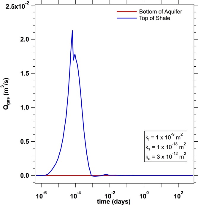
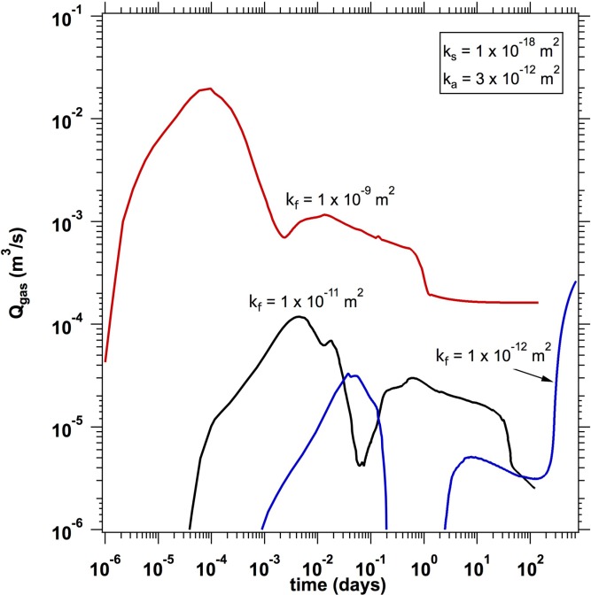
Figure 5 demonstrates the dominant role of the permeability k_f of the permeable feature (fracture and/or fault) connecting the TG reservoir and the aquifer, plotting Q_Gr and Q_Ga for k_f = 10⁻¹¹ m² and k_f = 10⁻¹² m² at the same base values of k_s and k_a. For both graphs, the y axes are split to resolve the much smaller values of Q_G. For k_f = 10⁻¹¹ m² (Figure 5a), the gas release at the top of the TG reservoir (i.e., at the mouth of the connecting fracture) begins within seconds of simulation startup, but it reaches a maximum value less than two orders of magnitude less than seen for k_f = 10⁻⁹ m². In Figure 5b, k_f = 10⁻¹² m², Q_Gr peaks at nearly another magnitude lower, despite the same fast onset of gas escape. Neither case allows gas to reach the base of the aquifer, nor the water well. Again, the gas stored in the hydraulic fracture appears to be the sole source of gas that can rise in the connecting fracture, as the matrix of the TG reservoir is unable to replenish it on short time scales.

Figure 5.

F-cases: Volumetric rates of gas transport to (i) the top of the reservoir (Q_Gr) and (ii) the base of the aquifer (Q_Ga) for the cases of (a) k_f = 10⁻¹¹ m² and (b) k_f = 10⁻¹² m²; with k_s = 10⁻¹⁸ m², k_a = 3 × 10⁻¹² m², L = L₁ = 200 m, and both the water and the gas wells producing. Note the split axes due to the difference in magnitude compared to Figure 4. CH₄ does not reach the aquifer base (Q_Ga = 0) either in a free gas phase or dissolved in the H₂O.

Figures 6 and 7 provide an illustration of the processes behind Figures 4 and 5b, respectively. For each, a 2-D color plot of the gas saturation (S_G) distribution is provided at the plane of the fracture at three different times. Note that, because the penetrating fracture scenario is represented as a half-space problem, the center of the fracture and the system is at y = 0. In Figure 6, the first plot, at t = 1.0 h, shows the initial breakthrough of water from the connecting fracture into the fracture within TG reservoir (−400 m < z < −300 m). In the second plot, at t = 12 h, enough water has entered the fracture that the bottom 25 m of the fracture has filled with the water from the connecting fracture (to S_G = S_ir,G). The inflow of water continues, and in the third plot, at t = 10 days, the water has risen to the level of the shale well at z = −350 m (at y = 0). Thus, water may begin to enter the shale well, and indeed by t = 10 days, the rate of water production at the shale well has reached a constant value of 0.86 kg/s. Thus, once a connection between the TG reservoir and the aquifer is established and the initial amount of stored gas is exhausted either through rise to the aquifer or through production by the gas well, further gas production may be severely impeded by continuous production of water cascading through the connecting fracture.

Figure 6.

F-cases: Gas phase saturation (S_G) in the plane of the connecting fracture at t = 1.0 h, t = 12 h, and t = 10 days, depicting a scenario characterized by limited gas phase flow through the connecting fracture, but significant downward flow of water into the aquifer, for k_f = 10⁻⁹ m², k_s = 10⁻¹⁸ m², k_a = 3 × 10⁻¹² m², L = L₁ = 200 m, and both the water and the gas wells are producing. Note that the fracture fills with water to the level of the producing shale well at z = −350 m. White boxes show the extent of the aquifer, pathway, and TG reservoir.

Figure 7.

F-cases: Gas phase saturation (S_G) in the plane of the connecting fracture at t = 1 day, t = 30 days, and t = 150 days, depicting a scenario that is characterized by minimal gas phase flow into the connecting fracture, and slow downward flow of water into the aquifer, for k_f = 10⁻¹¹ m², k_s = 10⁻¹⁸ m², k_a = 3 × 10⁻¹² m², L = L₁ = 200 m, and both the water and the gas wells are producing. White boxes show the extent of the aquifer, pathway, and TG reservoir.

The illustration in Figure 7 shows an otherwise identical system differing only in the value of k_f = 10⁻¹¹ m². Over the course of 150 days, we see slow flooding of the fracture in the TG reservoir with water from the penetrating fracture, but the invasion is slower due to the reduced permeability of the fracture pathway. By t = 30 days, we see the water reaching the shale well at z = −350 m, and by t = 150 days, the lower 10 m of the fracture has filled with water. In this case, water begins to be produced at the shale gas well by t = 100 days, but does not exceed a rate of 5 × 10⁻⁴ kg/s during the 2 years simulation time.

Figure 8 shows the dramatic increase in water production resulting from permeable pathways connecting to an overlying aquifer during production from the TG reservoir, plotting Q_ww for k_f = 10⁻⁹ m², k_f = 10⁻¹¹ m², and k_f = 10⁻¹² m² at the same base values of k_s and k_a. This represents water production from a 100 m segment of the horizontal well (the stencil described in section 4). The consequences of an induced fracture intercepting or creating a permeable pathway to an aquifer are notable: water production at the well goes from trace amounts (for a situation where flowback fluids have been removed prior to production) to much larger values as the inflow of water reaches the producing gas well. For the highest-k fracture pathways, the value is large (∼3.5 kg/s or nearly 2000 BBL/day contributed by the pathway). Reducing the permeability of the pathway by two or three orders of magnitude reduces the rate of water production proportionally, and delays the appearance of the nonformation water at the TG well. As such, undesired connectivity via permeable pathways if not discovered during the stimulation operation, are likely to have noticeable effects on production, once initiated. Lower-permeability pathways, however, may have less noticeable effects during early production.

Figure 8.

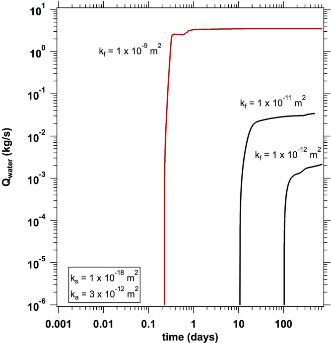
F-cases: Mass rate of water production (Q_ww) for a 100 m interval of the TG well for the cases of k_f = 10⁻⁹ m², k_f = 10⁻¹¹ m², and k_f = 10⁻¹² m², with k_s = 10⁻¹⁸ m², k_a = 3 × 10⁻¹² m²; L = L₁ = 200 m, and both the water and the gas wells producing.

CH₄ Release and Transport: L = L₂ = 800 m

Figure 9 shows the evolution of Q_Gr for a system similar to that of Figure 4, from which it differs only in the TG reservoir-to-aquifer separation that is now L = L₂ = 800 m. Because of the higher pressure in the deeper TG reservoir in this case, which results in a gas density about 2.5 larger than that in the L = L₁ = 200 m case, a significantly larger mass of the CH₄ stored in the hydraulic fracture. For the highest permeability, we do not observe a slight delay in the sharp decline in Q_Gr that is indicative of the CH₄ exhaustion during the 2 year duration of monitoring in this study, and a more gradual decrease. This is the result of both CH₄ depletion and of the reduction in effective permeability during the water and gas counterflow (as gas ascends and water drains through the connecting and the hydraulic fractures). For lower permeabilities, we see similar delays, but also the same order-of-magnitude decreases in Q_Gr, similar to that seen in Figure 5. An except is the blue curve in Figure 9, for k_f = 10⁻¹² m², where at t > 200 days the rate of gas transport out of the reservoir, Q_Gr, begins to increase and approach the magnitude seen at the most permeable configuration. For this case, gas also reaches the bottom of the aquifer, although Q_Ga < 10⁻⁶ m³/s for the 2 year timeframe shown in the graph.

Figure 9.

F-cases: Volumetric rates of gas transport to (i) the top of the reservoir (Q_Gr) for the base cases of k_f = 10⁻⁹ m², 10⁻¹¹ m², 10⁻¹² m², with k_s = 10⁻¹⁸ m², k_a = 3 × 10⁻¹² m², L = L₂ = 800 m, and both the water and the gas wells producing. Gas transport at the base of the aquifer (Q_Ga) is zero or less than 10⁻⁶ m³/s for all cases.

What is particularly interesting is that gas arrival at the aquifer base (as quantified by Q_Ga) remains zero during the entire monitoring period for the two highest permeabilities, and thus no CH₄ reaches the aquifer. This indicates that, despite the larger CH₄ mass that is initially available in the hydraulic fractures, the long length of the connecting fractures makes possible the dissolution of the ascending CH₄ in the gas phase into the descending aqueous phase, which is eventually removed through the gas well in the TG reservoir. For the lowest fracture permeability, k_f = 10⁻¹² m², however, trace amounts of CH₄ reach the bottom of the aquifer via the pathway at 278 days, but Q_Ga remains at very low rates (Q_Ga < 10⁻⁶ m³/s) within the 2 year timeframe.

Parametric Variations in the F-Case Studies

The large number of transport simulations result in hundreds of methane flux curves, many of which are very much alike in pattern, shape, and features (arrival times, maximum fluxes). To summarize the results concisely, we now present a statistical analysis of the complete ensemble of connecting-fracture/fault simulations. By comparing key metrics (gas phase arrival and the corresponding times) versus key parameters, we can explore the envelope of possible scenarios and evaluate the importance of various geological parameters to the CH₄ release, transport and production in the TG reservoir-overburden-aquifer continuum, thus gleaning a measure of the associated potential environmental impact on shallow groundwater.

Figures 10 and 11 present percentages of simulations that result in arrival of gas-phase methane at the base of the aquifer versus production strategy and the exponent of the three permeability parameters, i.e., k_f, k_s and k_a. The statistics are assessed independently for the two separations, L = L₁ = 200 m and L = L₂ = 800 m. Thus, each bar represents the percentage of simulations that show the appearance of free gas phase at the base of the aquifer when a particular parameter has a fixed value in a system (a) with the same separation L and (b) with all combinations of the other parameters varied. Note that the total number of simulations for each separation L is N_FL = 72.

Figure 10.

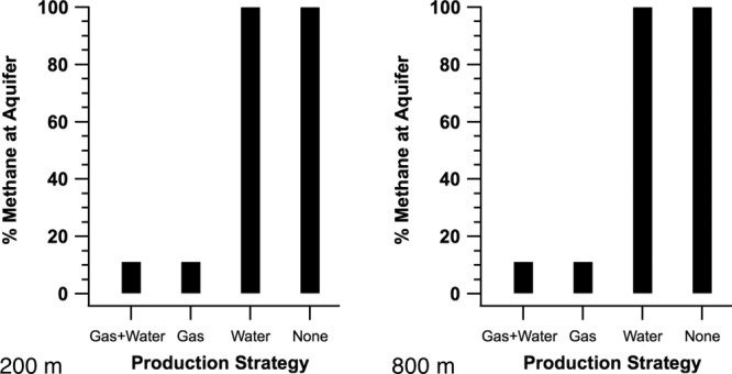
F-cases: Percentage of the penetrating fracture/fault scenarios that result in gas arrival at the base of the aquifer, as a function of the production strategy for (a) L = L₁ = 200 m and (b) L = L₂ = 800 m; (N_FL1 = 72, N_FL2 = 72).

Figure 11.

F-cases: Percentage of the penetrating fracture/fault scenarios that result in gas arrival at the base of the aquifer, as a function of k_f, k_s, and k_a. (top) L = L₁ = 200 m, and (bottom) L = L₂ = 800 m (N_FL1 = 72, N_FL2 = 72).

The figures suggest that for the penetrating fracture scenarios (a) the key parameter that affects the evolution of CH₄ gas at the base of the aquifer is the production strategy, and (b) the permeabilities k_f, and k_s of the fracture and TG reservoir respectively, show a much weaker correlation. Aquifer permeability k_a shows no correlation. While initially counterintuitive, it is clear that the low fracture volume and the low-k gas-bearing shale results in a limited volume of gas available for short-term release. When the gas well is producing (at constant pressure, and initially at high rates), the driving force of buoyancy of the methane is countered by the rapid depressurization of the small fracture volume. This reduces the favorability of pressure gradients that regulate the buoyant transport of the gas, and also drives a downward flow of water from the aquifer via the connecting fracture that is likely to dissolve and transport downward much of the methane that has escaped the TG reservoir. Without the producing shale gas well, the gas may rise via buoyancy with any downward-flowing water displacing any gas that has left the reservoir. This illustrates the importance of the producing gas well in the reduction of the gas stored in the hydraulic fracture. As already discussed, this is the main source of gas available to escape through the connecting fracture because of the inability of the matrix to significantly replenish in short timeframes. Hydraulically fractured systems may be shut in for short time periods after fracturing operations and therefore, if a permeable out-of-formation pathways have been formed, gas migration potential may be increased during the shut-in time. Also seen in Figure 11 is a slightly higher chance of gas escape for the lowest fracture permeability, k_f = 10⁻¹² m². Close examination of individual simulation results reveals that the lower permeability delays the downward flow of freshwater and rapid-reequilibration of the connecting fracture with the fracture in the TG reservoir. As a result, trace amounts of gas that enter in the connection fracture at early times are able reach the top of the connecting fracture before downward flows become significant, but the gas release is not at large enough rates to result in free gas in the aquifer (100% dissolution near the fracture-aquifer interface). Finally, another correlation worth examining in Figure 11 is the slight increase in the likelihood of gas release with the highest-k shale, k_s = 10⁻¹⁸ m². Here the additional permeability in the shale slightly reduces the rate of depressurization of the fracture in the TG reservoir (via short-term gas migration from the shale matrix into the fracture and wellbore).

Figure 12 presents scatterplots of CH₄ gas arrival times at the aquifer base and at the water well versus k_f, k_s and k_a, using different symbols for L₁ and L₂ separation. For both separations, the arrival times are clearly dependent on k_f, as would be expected—the rate of transport through a feature is a function of distance and fracture permeability. For L = L₁, the breakthrough times at the base of the aquifer vary from a few minutes to up to 40 days, and for L = L₂, the breakthrough times vary between 30 min to over 300 days. This is important to note, because although breakthrough likelihood does not show a strong correlation with permeability in Figure 11, this is partly a consequence of the particular geometries chosen. The huge variation in breakthrough times seen in Figure 12 indicates that for many possible systems and scenarios, k_f, by regulating the rate of breakthrough, will thus regulate the possibility of breakthrough, as breakthrough is governed by a set of complex coupled flow-transport processes. For example, slower movement of gas through a connecting fracture means more time for downward-flowing water to fully dissolve the gas.

Figure 12.

F-cases: Scatterplots of gas arrival time at the base of the aquifer versus key permeabilities in the F-base cases. The “cross” symbol corresponds to L = L₁ = 200 m, and the “plus” symbol corresponds to L = L₂ = 800 m.

We cannot identify any obvious correlation between gas breakthroughs and k_s and k_a, although some later breakthrough times occur for higher k_s. Examination of the individual runs indicates that these late-breakthrough case may be artifacts of the 2 year simulation limit in this study, such that additional scenarios with low k_f and high k_s may also eventually show late breakthrough when taken to longer times. In fact, these two late breakthroughs account for the slight increase in the likelihood of breakthrough for k_f = 10⁻¹² m² seen in Figure 11. These longer-term migration patterns will be investigated in follow-up studies.

Figure 13 explores the dependence of breakthrough times (at the aquifer base and at the water well) on L and the production strategy. Unsurprisingly, a thinner overburden allows faster breakthrough times, and here the differences appear to cluster in groups that suggest slightly less than an order-of-magnitude difference resulting from 4X the connection feature length. In the second plot, the effect of the production strategy is pronounced. With a producing gas well, there are only a few instances of rapid breakthrough for L = L₁ = 200 m, and fewer breakthroughs overall. Without gas production, the range of breakthrough times tends toward fast breakthrough, ranging from rapid (minutes) to 20 days. Production strategy is clearly a key determiner of gas-release, and this figure, along with Figure 0, suggests a low likelihood of gas escape to overlying aquifers if production begins immediately after the penetrating fracture is formed for cases with initial hydrostatic equilibrium.

Figure 13.

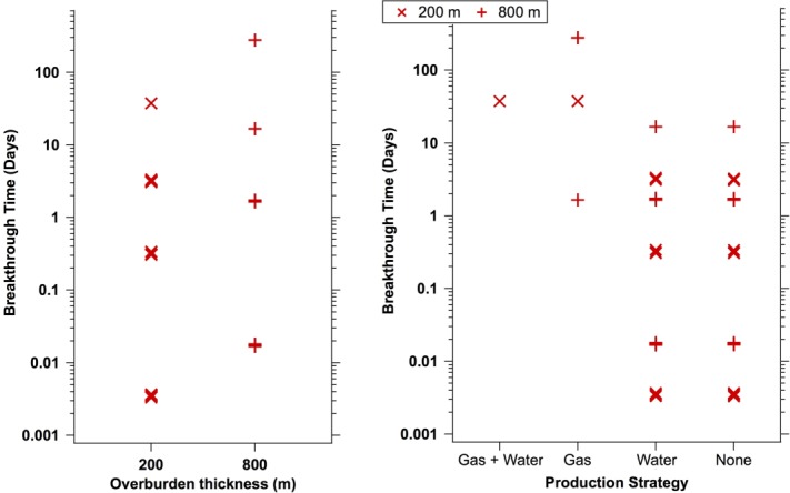
F-cases: Scatterplots of CH₄ gas arrival time at the base of the aquifer versus L and production strategy. The “cross” symbol corresponds to L = L₁ = 200 m, and the “plus” symbol corresponds to L = L₂ = 800 m.

W-Base Cases: Transport Through Deteriorating Wells

CH₄ Release, Transport and Production: L = L₁ = 200 m, k_w = 10⁻⁹ m²

Figure 14 shows the volumetric flow rates of the free gas phase (practically 100% CH₄, with traces of H₂O vapor) arriving at the top of TG reservoir (Q_Gr, blue curve), and at the base of the aquifer (Q_Ga, red curve). In this case, k_w = 10⁻⁹ m² (=1000 D), k_s = 10⁻¹⁸ m², k_a = 3×10⁻¹² m², L = L₁ = 200 m, and both the gas and the water well are producing. The instantaneous exit of gas through the top of the TG reservoir via the deteriorated well (for reasons already explained in section 5.1.1) is described by the Q_Gr curve, which, after the initial maximum at t = 3 s, decreases quickly, albeit with fluctuations caused by the effects of two-phase flow of the counterflowing gas (ascending) and water (descending) in the connecting offset well. For Q_Ga, CH₄ gas arrives at the base of the aquifer at t = 7 min, but at a much lower rate than seen leaving the TG reservoir. This quick breakthrough is because of the gas buoyancy, the relatively short separation L and the limited pore volume of the permeable pathway (which, at k_w = 10⁻⁹ m², indicates either voids caused by separation between the cement and the casing or formation, or breached tubing). After this initial breakthrough, Q_Ga decreases to negligible values by t = 7 h because of the depletion of the gas source (the hydraulic fracture), the depressurizing effect of the producing gas well, and the dissolution of gas by the downward-flowing aquifer water through the deteriorated well.

Figure 14.

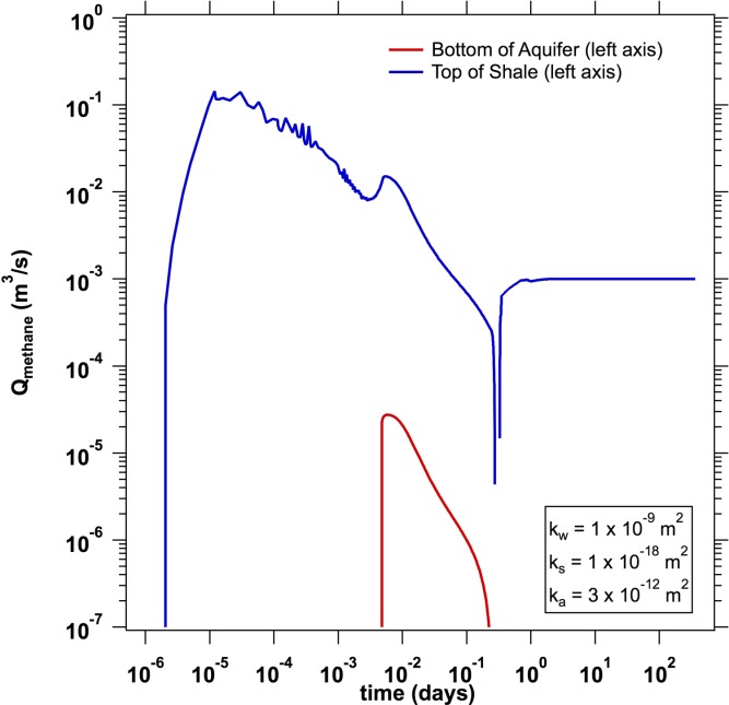
W-cases: Volumetric rates of gas transport to (i) the top of the reservoir (Q_Gr) and (ii) the base of the aquifer (Q_Ga) for the base case of k_w = 10⁻⁹ m², with k_s = 10⁻¹⁸ m², k_a = 3 × 10⁻¹² m²; L = L₁ = 200 m, with both the gas and the water well producing.

The difference between the presence of the Q_Ga curve in Figure 14, and its absence in the corresponding Figure 4 of the F-cases, is attributed to the much lower pore volume of the connecting well pathway (compared to that of a connecting fracture in Figure 4), which reduces the possible gas storage in the connecting features, increases the speed at which buoyancy alone drives flow (as the system is initially hydrostatic), and enhances the possibility of CH₄ appearance at the aquifer base. Comparing the Q_Gr curve in Figure 14 to Figure 4 also highlights some differences between the two types of connecting feature. Q_Gr for the W-case peaks at rates seven times that of the F-case with all other parameters equal, and gas flow out of the reservoir continues for hours rather than only minutes. This is also function of the difference in total volume between the void spaces of two pathways of equal length but different geometry—in fact the total pore volume of the penetrating offset well is about 5X less than the volume of the connecting fracture as-meshed. Finally, the offset geometry of the wall also separates the connecting feature from the horizontal shale well, allowing more gas to enter the connecting feature via buoyancy before the rapid depressurization of the fracture establishes a downward flow regime. Thus, for otherwise identical reservoir-aquifer configurations, the W-case shows a greater potential for gas release, all other parameters equal.

As the importance of production strategy has already been highlighted for the F-cases, we expect it to be a factor in the W-cases as well, and Figure 15 confirms this. Figure 15 plots the volumetric flow rates Q_Gr and Q_Ga for a case with k_w = 10⁻⁹ m² (=1000 D), k_s = 10⁻¹⁸ m², k_a = 3×10⁻¹² m², L = L₁ = 200 m, but in comparison to Figure 14, only the water well is producing. We see in this figure both the importance of production strategy, but also the degree to which gas release is a limited, short-term process. Gas exiting the top of the reservoir, Q_Gr, peaks rapidly above 0.5 m³/s, and maintains significant values for roughly 40 min before dropping to a very low (insignificant over shorter times) level. The gas reaches the aquifer in under 3 min, and peaks at flow rate 7X that which was seen in Figure 14, where no gas well was producing. However, this flow drops off rapidly and drops below significance (and eventually to zero) at the same time gas stops exiting the TG reservoir. Some of the released CH₄, in fact, is likely to return to the degraded well and head toward the reservoir, as aqueous flow is uniformly downward away from the aquifer for t > 4 min, thus providing an exit for the dissolved gas released into the aquifer.

Figure 15.

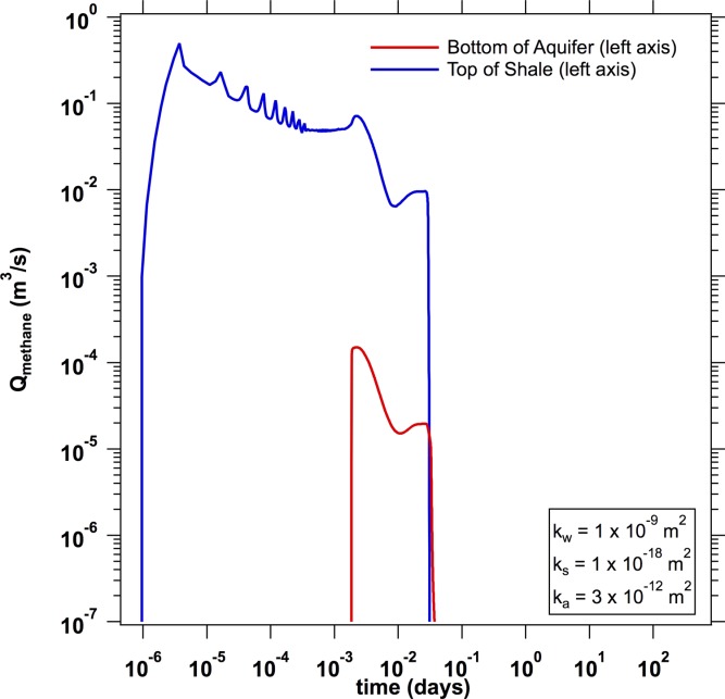
W-cases: Volumetric rates of gas transport to (i) the top of the reservoir (Q_Gr) and (ii) the base of the aquifer (Q_Ga), for the case of k_w = 10⁻⁹ m², with k_s = 10⁻¹⁸ m², k_a = 3 × 10⁻¹² m²; L = L₁ = 200 m, with only the water well producing.

CH₄ Release and Transport: L = L₁ = 200 m, k_w = 10⁻¹², 10⁻¹⁵ and 10⁻¹⁸ m²

Figure 16 compares the evolution of Q_Gr for k_w = 10⁻¹² m², which is representative of a well-fractured (deteriorating) cement or a small separation between the cement and the outermost casing, and k_w = 10⁻¹⁵ m², a competent, high-quality cement, to the previous case of k_w = 10⁻⁹ m². In both cases, both the water well and TG well are producing. The differences caused by the lower k_w (compared to that in Figure 14) are obvious. For k_w = 10⁻¹² m², Q_Gr shows rapid release of CH₄ gas from the TG reservoir into the connecting well, but no gas breakthrough at the base of the aquifer (Q_Ga). The release rate is orders of magnitude lower than for k_w = 10⁻⁹ m². Q_Gr reaches a low, steady-state value by t = 3 days with no evidence of (or mechanism for) increasing. For k_w = 10⁻¹⁵ m² (describing a competent, high-quality cement), Q_Gr shows some escape of gas, but its highest rate is about 2 orders of magnitude lower than that for k_w = 10⁻¹² m² and 6 orders of magnitude lower than that for k_w = 10⁻⁹ m², i.e., reflective of the permeability difference of the connecting well. This means no significant gas migration over the simulation timeframe (Q_Ga is zero), and it is likely that any possible migration would only occur over much longer time scales [see Gassiat et al., ²⁰¹³].

Figure 16.

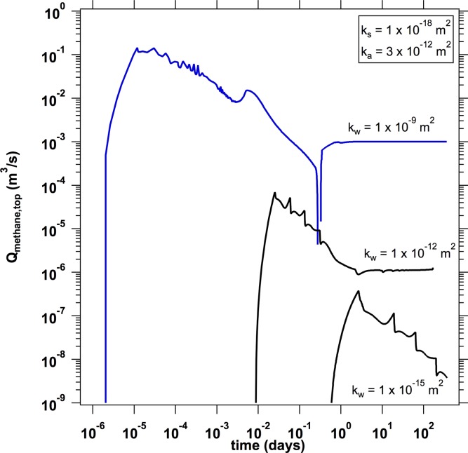
W-cases: Volumetric rates of gas transport to the top of the reservoir (Q_Gr) for the base cases of k_w = 10⁻¹² m² and k_w = 10⁻¹⁵ m² compared to that for k_w = 10⁻⁹ m², with k_s = 10⁻¹⁸ m², k_a = 3 × 10⁻¹² m²; L = L₁ = 200 m, and both the gas and the water well producing. Note that Q_Ga = 0 for all times for k_w = 10⁻¹² m² and k_w = 10⁻¹⁵ m² (no gas breakthrough at the aquifer).

For k_w = 10⁻¹⁸ m² (describing in essence a cement as permeable as an unfractured shale), Q_Gr is practically zero, as is Q_Ga, obviating the need for further simulations. This was entirely consistent with expectations, as such a k_w describes the permeability of the typical overburden isolating natural TG reservoirs that do not exhibit significant leakage over geologic time.

CH₄ Release and Transport: L = L₂ = 800 m

Figure 17 shows the volumetric flow rates of the free gas phase (practically 100% CH₄, with traces of H₂O vapor) arriving at the top of TG reservoir (Q_Gr), for k_w = 10⁻⁹ m² and k_w = 10⁻¹² m². Compared to Figure 16 (L = L₁ = 200 m), there are some significant differences, the most important of which is the much earlier exhaustion of the gas in the hydraulic fracture, seen as the falloff in the Q_Gr curve online minutes after simulation start. The fracture, as already discussed, is the sole source of gas available for transport in the short-term. Because of the much longer distance to cover (L₂ versus L₁) and thus the larger volume of the connecting pathway, the Q_Ga is zero, as the quantity of available free gas and the hydrostatic pressure regime (shifted by the producing shale gas well to evolve toward downward flow of water from the aquifer) prevents escape of gas into the aquifer. For k_w = 10⁻¹² m², the effect of the significant decrease in cement permeability is a 3 order-of-magnitude decrease in the rate of gas escape from the reservoir, Q_Gr, although this highly moderated release occurs over several days. No release into the aquifer is seen, nor would be expected due to the process discussed previously. Analogous to Figure 16, the cases of k_w = 10⁻¹⁵ m² and k_w = 10⁻¹⁵ m² with L = L₂ show only traces of gas entering the connecting feature at very low rates, and thus no escape of gas.

Figure 17.

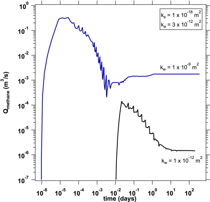
W-cases: Volumetric rates of gas transport to (i) the top of the reservoir (Q_Gr) and (ii) the base of the aquifer (Q_Ga) for the cases of k_w = 10⁻⁹ m² and k_w = 10⁻¹² m² with k_s = 10⁻¹⁸ m², k_a = 3 × 10⁻¹² m²; L = L₂ = 800 m, and both the gas and the water well producing. Note that Q_Ga = 0 for all times (no gas breakthrough at the aquifer).

Note that all L = L₂ systems have a larger initial quantity of gas stored in the fracture than the L = L₁ cases because the higher pressure at the deeper TG reservoir results in initial gas density about 2.5X higher than that for the shallower reservoir at L = L₁. Comparing Figure 17 to Figure 14, we see that the peak Q_Gr for L = L₂ is over twice that of L = L₁. Tracking of gas through the defined interfaces indicates that about twice as much gas leaves the reservoir and enters the connecting offset well for L₂ versus L₁, although the greater separation prevents escape to the aquifer (for reasons discussed previously, including a steady flow of undersaturated water flowing downward countercurrent to any rising gas).

Parametric Variations in the W-Case Studies

The statistical analysis presented here is the result of the large number of combinations and permutations of the W-cases, which make impractical the detailed discussion of all individual cases. The task is made easier by the distinct similarities of results from simulations with similar characteristics. The approach here follows that described in detail in section 5.1.3.

Figure 18 presents percentages of simulations that result in arrival of gas-phase methane at the base of the aquifer versus the exponent of the three permeability parameters, i.e., k_w, k_s and k_a. The percentages for the two separations, L = L₁ = 200 m and L = L₂ = 800 m, are shown in the top and bottom line of plots, respectively. Figure 18 clearly demonstrates that (a) the only important parameters that affect the evolution of CH₄ gas at the base of the aquifer is the permeability k_w of the connecting well, and (b) the separation L. The permeabilities k_s and k_a of the TG reservoir and of the aquifer appear to be inconsequential. Thus, all cases with k_w = 10⁻⁹ m² show gas at the base of the aquifer, with the probably reduced by 50% for the larger value of L = 800 m. For k_w = 10⁻¹² m², half of the cases show gas at the aquifer for L = 200 m, and no cases release gas for L = 800 m. These statistics reflect the effects of permeability and separation discussed in the previous section.

Figure 18.

W-cases: Percentage of the penetrating fracture/fault scenarios that result in gas arrival at the base of the aquifer, as a function of k_w, k_s, and k_a. The top row is for L = L₁ = 200 m, and the bottom row is for L = L₂ = 800 m (N_WL1 = 96, N_WL2 = 96).

Figure 19 shows the likelihood of CH₄ gas appearance at the aquifer base versus L and the production regime/strategy. Here we see the factors driving the difference between L = 200 m and L = 800 m as noted in Figure 18. For L = L₁ = 200 m, a producing TG well reduces the chance of gas at the aquifer by preventing cases with k_w = 10⁻¹² m² from releasing gas (i.e., only k_w = 10⁻⁹ m² cases release gas). For L = L₂ = 800 m, a producing TG well eliminates the chance of any gas escape for any of the permeabilities studied. Only systems without the mitigating feature of a producing TG well are able to transport gas to the aquifer. As seen in the W-cases, production in the TG reservoir is clearly a large mitigating factor when estimating the likelihood of gas escape.

Figure 19.

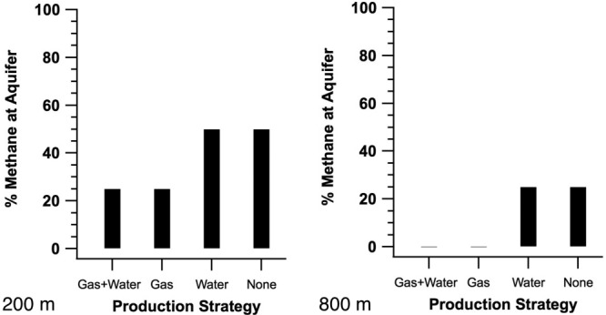
W-cases: Percentage of the connecting offset well scenarios that result in gas arrival at the base of the aquifer versus production strategy for (left) L = L₁ = 200 m and (right) L = L₂ = 800 m (right); (N_WL1 = 96, N_WL2 = 96).

Figure 20 is a scatterplot of CH₄ gas arrival times at the aquifer base versus k_f, k_s and k_a, using different symbols for L₁ and L₂ separations. Confirming the earlier observations, the only safe conclusion that can be gleaned from this set of graphs is that the only important factor is k_w, with the results of variation in all other permeability parameters appearing minimal to inconsequential.

Figure 20.

W-cases: Scatterplots of gas arrival time at the base of the aquifer versus key feature permeabilities. “Cross” symbol corresponds to a separation of 200 m, while “plus” symbol corresponds to 800 m separation.

Figure 21 explores the dependence of breakthrough times (at the aquifer base) on L and the production strategy, and is slightly more informative. A larger L is associated with slightly longer arrival times at the base of the aquifer, but no such relationship is obvious for CH₄ arrival at the water well. The effect of production strategy is to either allow or prevent gas breakthrough for L = 200 m, and for L = 800 m the breakthrough times are not greatly affected when the gas is able to escape to the aquifer.

Figure 21.

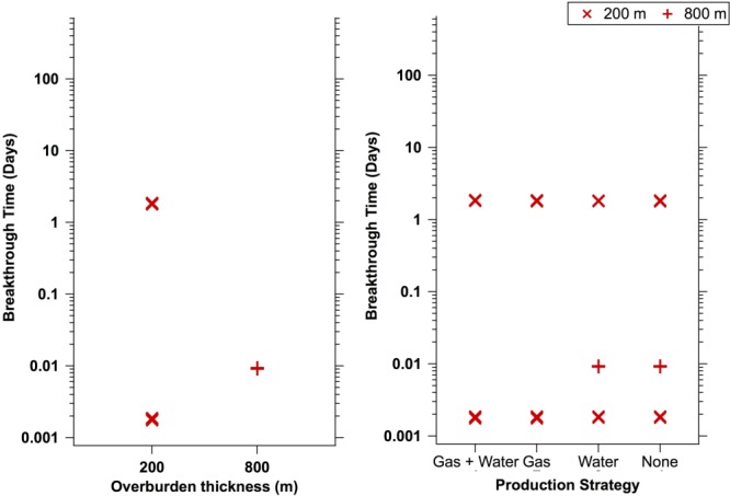
W-cases: Scatterplots of gas arrival time at the base of the aquifer versus overburden thickness and production strategy. “Cross” symbol corresponds to a separation of 200 m, while “plus” symbol corresponds to 800 m separation.

Direction of Aqueous Phase Flow and Effect of the Pressure Regime of the TG Reservoir

The results of our study indicate that, except for a brief initial period of upward flow during the initial phase of rapid gas ascent in the connecting feature (if such gas is present), water flow is uniformly downward after gas migration has slowed and breakthrough occurs. We identified only a very limited number of cases associated with nonnegative flows through the connecting feature, and some of these are related to systems with low permeability of the connecting feature, which results in very slow rise of fluids that do not reach the aquifer base within simulation time. Other examples are low-k configurations where upward fluid flow rates exist but never exceed ∼10⁻⁷ kg/s or less than 10 kg of water transport per year, essentially inconsequential in terms of short and medium-term transport. The long-term fate of these incomplete-breakthrough cases will be examined in a future study. This trend of downward flow continues through the 2 year simulation period, and is most (understandably) more pronounced when the gas well is operating. However, in cases where the gas well is not operation (and also in cases where neither the gas nor water well is operating), we still observe a consistent trend toward downward aqueous flow. One driving force that appears to be at work is the phenomenon of imbibition into the undersaturated shale matrix [Engelder, ²⁰¹⁴]. As our initial conditions assume gas-filled fractures in the TG reservoir and no leak-off into the shale of hydraulic fracturing fluids, the thin layer of shale adjacent to the fracture is able to absorb the downward-flowing water entering the TG through the permeable connecting feature. A close examination of the shale gridblocks adjacent to the fracture (particularly when such elements are adjacent to a “flooded” zone as see in Figure 7) shows an increase in aqueous saturation (S_a) with time. This phenomenon only affects a thin layer of shale within the simulation timeframe, but the large surface area of the fracture (60,000 m²) means that a slight increase in S_a in the shale adjacent to the fracture could represent a significant sequestration of water and a noticeable driving force for downward fluid flow. Longer simulations, occurring as part of the EPA study and a future paper, will examine this behavior over longer timeframes.

Effect of Gas Sorption

We compared results from several F-cases and W-cases simulation with and without gas sorption, i.e., with the TG reservoir simulated as a shale-gas and a tight-sand reservoir, respectively. Without exception, the results were practically identical. This observation is consistent with the findings in this study, which indicate that gas releases from a TG reservoir connected to a shallower aquifer by a permeable feature (fracture or well) are largely limited to the initial content of the hydraulically induced fractures, with further gas releases (supplied by gas release from sorption) limited over short timeframes due to low permeabilities. The insignificance of sorption in this study is further reinforced by the results of earlier studies [Freeman et al., ²⁰¹³], which have demonstrated that the effect of sorption (as measured by its contribution) is minimal during the early stages of production from stimulated shale-gas reservoirs. Furthermore, the imbibition of water into the shale adjacent to the fracture wall would reduce the effective permeability of the shale and thus further reduce communication between the fracture and the shale matrix, reduce gas flow from the shale, and reduce the rate of recharge of the fracture. It should be noted that this behavior is for hydrostatic conditions, and overpressured reservoirs (to be simulated in future publications) may exhibit different behavior.

Summary, Conclusions, and Comments

We investigated gas and water transport between a deeper (200 m or 800 m separation) TG reservoir and a shallower overlying freshwater aquifer following hydraulic fracturing (stimulation) operations. Such transport can only occur if there is failure of the overburden, which we investigated in two general categories. In the first (F-cases), communication between the reservoir and the aquifer is established by a connecting fracture and/or a permeable fault tied to the hydraulic fracture. In the second (W-cases), the connecting feature is an offset unsealed well (often abandoned) with deteriorated casings, imperfect cement (weak, fractured, and/or incompletely sealing the annular space) and even (possibly) tubing.

We draw the following conclusions from this study:

1. After evaluating a number of factors that could potentially affect the transport of gas to shallower aquifers (with the consequent environmental concerns) following hydraulic fracturing operations, we determined that, in the F-cases, the main factors affecting the transport of gas to the base of the aquifer and its appearance at a producing water well in the aquifer are (a) the production regime, i.e., an active gas well in the TG reservoir mitigates release, (b) the permeability k_f of the connecting fracture, and less so, (c) the separation L between the TG reservoir and the aquifer.

2. Similarly, in the investigation of the behavior of the W-cases we determined that the main factors (by far) affecting the transport of gas to the base of the aquifer and its appearance at a producing water well in the aquifer are the permeability k_w of the connecting offset well, and the production regime (i.e., whether a gas well in the TG reservoir is active). Permeabilities k_w <= 10⁻¹⁵ m² lead without exception to no gas arrivals at the aquifer for L as small as 200 m, and only the highest permeability leads to a large probability of release for all other parameters, and for larger separations, a producing TG well can mitigate release even for such high permeabilities. Generally speaking, gas transport through such a connecting feature conveys larger CH₄ amounts to the aquifer than the connecting fractures/faults of the F-cases. This is caused by the lower pore volume of the connecting features in the W-cases, which results in limited gas storage within the connecting feature.

3. The TG reservoir appears unable to recharge the hydraulic fracture over short time scales for a hydrostatic pressure regime and an unfavorable evolution of relative permeability. Thus, the amount of gas available for immediate migration toward the shallower aquifer is limited to that initially stored in the hydraulically induced fractures immediately after the conclusion of the stimulation process and prior to the beginning of gas production. A direct consequence of this is that the period of significant gas (originating from the TG reservoir) presence in the aquifer is limited. This appears to be true even in cases where a TG well is not producing and gas in the fracture is not being consumed during such production. Such “free” release via buoyancy effects may be larger in magnitude, but still small in total volume and limited in duration.

4. The dependence on production strategy is of particular interest because in the field, stimulation may not necessarily be followed immediately by production, and production may not be continuous (i.e., well shut-in). However, the opening of a highly permeable pathway is also likely to deliver significant quantities of water to the producing well, which would hamper gas production and provide a clear notice of the presence of such a pathway.

5. Aqueous flow in nearly all of our parametric cases is downward, with the exception of systems with very low permeability of the connecting features or exhibiting incomplete gas migration at the end of simulation time. This is true whether or not a TG well is producing and thus creating a downward driving force. Additional long-term studies are needed to conclusively address the issue, including studies of overpressured reservoirs.

   These conclusions must be viewed in light of the limitations and assumptions of this study, which include:

6. In this study, we do not address the possibility of the various failure scenarios, neither do we assess the probability of their occurrence. Such assessments are clearly indispensable for a thorough evaluation of the problem, but are not yet possible because of lack of sufficient data. Thus, in the contaminant transport studies we considered pathways between the TG reservoir and a shallow aquifer a given and aimed to determine the extent of the gas and water transport covering a spectrum of system properties and production conditions. The scenarios that result in rapid release of gas are also scenarios that require the formation of pathways with consistent, high permeability, and the mechanisms for forming such pathways must be determined. For example understanding the relative probability of out-of-zone fracturing or fault activation versus interception of highly degraded, abandoned wells would put the hazards into proper context.

7. The initial pressure distribution throughout the system is hydrostatic. Overpressured systems are likely to exhibit different behavior—although an undersaturated shale is likely to enhance gas migration to a greater degree than liquid migration. This phenomenon will be investigated in a subsequent study.

8. The study of the F-cases in our simulations presupposes the existence of a continuous connecting permeable feature (natural fractures or permeable faults tied to hydraulically induced fractures), without considering the probability or even possibility of such occurrences. This is an important assumption because the creation or existence of such features cannot be ascertained on current evidence. The formations between the TG reservoir and aquifer are assumed to be otherwise impermeable.

9. The importance of gathering reliable field and laboratory data to constrain the factors dominating the system performance cannot be overemphasized.

Continuing work in this area must include longer simulation timeframes, to assess migration potential within the aquifer, additional parametric variations, including greater separations L for the most permeable systems, and variations in penetrating well offset, including the possibility of the production well serving as a communication pathway (i.e., via the annulus or degraded cement). These studies must also include the case of overpressured reservoirs, since such formations seem like a plausible mechanism that could increase the flow of gas to the aquifer, and counter the effects of imbibition and the observation of a downward trend in aqueous flow. This is important to explore the upper end of release potential and to determine what combination of factors would be required to drive significant gas and reservoir liquids into freshwater aquifers, and whether such release can impact groundwater resources or result in the appearance of gas at nearby producing water wells. These cases, and the corresponding simulations, will be the subject of a forthcoming paper.

References

- American Petroleum Institute (API) Policy Issues: Facts About Shale Gas 2014. 2014. . [Available at http://www.api.org/policy-and-issues/policy-items/exploration/facts_about_shale_gas.]
- Bachu S. Valencia RL. Well integrity challenges and risk mitigation measures. The Bridge. Natl. Acad. Eng. 2014;44(2):28–33. [Google Scholar]
- Barree RD. Conway MW. 2007. Multiphase non-Darcy flow in proppant packs, SPE 109561, Proc. SPE 2007 Annual Technical Conference and Exhibition, Anaheim, Calif., 11–14 Nov.
- Brantley SL, Yoxtheimer D, Arjmand S, Grieve P, Vidic R, Pollak J, Llewellyn GT, Abad J. Simon C. Water resource impacts during unconventional shale gas development: The Pennsylvania experience. Int. J. Coal Geol. 2014;126:140–156. doi: 10.1016/j.coal.2013.12.017. [Google Scholar]
- Crow W, Carey JW, Gasda S, Brian Williams D. Celia M. Wellbore integrity analysis of a natural CO2 producer. Int. J. Greenhouse Gas Control. 2010;4(2):186–197. [Google Scholar]
- Davies RJ, a. Mathias S, Moss J, Hustoft S. Newport L. Hydraulic fractures: How far can they go? Mar. Pet. Geol. 2012;37:1–6. doi: 10.1016/j.marpetgeo.2012.04.001. [Google Scholar]
- Davies RJ, Almond S, Ward RS, Jackson RB, Adams C, Worrall F, Herringshaw LG, Gluyas JG. Whitehead MA. Oil and gas wells and their integrity: Implications for shale and unconventional resource exploitation. Mar. Pet. Geol. 2014;56:239–254. [Google Scholar]
- Dusseault M. Jackson R. Seepage pathways assessment for natural gas to shallow groundwater during well stimulation, in production, and after abandonment. Environ. Geosci. 2014;21(3):107–126. doi: 10.1306/eq.04231414004. [Google Scholar]
- Engelder T, Cathles LM. Bryndzia LT. The fate of residual treatment water in gas shale. J. Unconventional Oil Gas Res. 2014;7:33–48. [Google Scholar]
- Fisher K. Warpinski N. Hydraulic-fracture-height growth: Real data. SPE Prod. Oper. 2012;27(1):8–19. [Google Scholar]
- Flewelling SA. Sharma M. Constraints on upward migration of hydraulic fracturing fluid and brine. Ground Water. 2014;52:9–19. doi: 10.1111/gwat.12095. doi: 10.1111/gwat.12095. [DOI] [PMC free article] [PubMed] [Google Scholar]
- Flewelling SA, Tymchak MP. Warpinski N. Hydraulic fracture height limits and fault interactions in tight oil and gas formations. Geophys. Res. Lett. 2013;40:3602–3606. doi: 10.1002/grl.50707. [Google Scholar]
- Freeman CM, Moridis GM. Blasingame TA. A numerical study of microscale flow behavior in tight gas and shale gas reservoir systems. Transp. Porous Media. 2011;90(1):253–268. [Google Scholar]
- Freeman CM, Moridis GM, Ilk D, Blasingame TA. A numerical study of performance for tight gas and shale gas reservoir systems. J. Pet. Sci. Eng. 2013;108:22–39. , doi: 10.1016/j.petrol.2013.05.007. [Google Scholar]
- Freeman CM, Boyle KL, Reagan MT, Johnson JN, Rycroft C. Moridis GJ. MeshVoro: A three-dimensional voronoi mesh building tool for the TOUGH family of codes. Comput. Geosci. 2014;70:26–34. [Google Scholar]
- Gasda SE, Celia MA, Wang JZ. Duguid A. Wellbore permeability estimates from vertical interference testing of existing wells. Energy Procedia. 2013;37:5673–5680. [Google Scholar]
- Gassiat C, Gleeson T, Lefebvre R. McKenzie J. Hydraulic fracturing in faulted sedimentary basins: Numerical simulation of potential contamination of shallow aquifers over long time scales. Water Resour. Res. 2013;49:8310–8327. doi: 10.1002/2013WR014287. [Google Scholar]
- Hill DG. Nelson CR. Gas productive fractured shales: An overview and update. Gas TIPS. 2000;6(3):4–13. [Google Scholar]
- Jackson RB, Vengosh A, Darrah TH, Warner NR, Down A, Poreda RJ, Osborn SG, Zhao K. Karr JD. Increased stray gas abundance in a subset of drinking water wells near Marcellus shale gas extraction. Proc. Natl. Acad. Sci. U. S. A. 2013a;110(28):11,250–11,255. doi: 10.1073/pnas.1221635110. doi: 10.1073/pnas.1221635110. [DOI] [PMC free article] [PubMed] [Google Scholar]
- Jackson RE, Gorody AW, Mayer B, Roy JW, Ryan MC. Van Stempvoort DR. Groundwater protection and unconventional gas extraction: The critical need for field-based hydrogeological research. Ground Water. 2013b;51(4):488–510. doi: 10.1111/gwat.12074. doi: 10.1111/gwat.12074. [DOI] [PubMed] [Google Scholar]
- Kim J. Moridis GJ. 2012. , and ), Gas Flow tightly coupled to elastoplastic geomechanics for tight and shale gas reservoirs: Material failure and enhanced permeability, Proc. SPE Americas Unconventional Resources Conference, Pittsburgh, Pa.
- Kim J. Moridis GJ. Development of the T+M coupled flow–geomechanical simulator to describe fracture propagation and coupled flow–thermal–geomechanical processes in tight/shale gas systems. Comput. Geosci. 2013;60:184–198. [Google Scholar]
- Kim J, Um ES. Moridis GJ. 2014. Fracture propagation, fluid flow, and geomechanics of water-based hydraulic fracturing in shale gas systems and electromagnetic geophysical monitoring of fluid migration, SPE 168578, Proc. SPE Hydraulic Fracturing Technology Conference, Woodlands, Tex.
- King GE. 2012. Hydraulic fracturing 101: What every representative, environmentalist, regulator, reporter, investor, university researcher, neighbor and engineer should know about estimating frac risk and improving frac performance in unconventional gas and oil wells, paper SPE 152596 presented at Hydraulic Fracturing Technology Conference, Soc. of Pet. Eng., Woodlands, Tex.
- Kissinger A, Helmig R, Ebigbo A, Class H, Lange T, Sauter M, Heitfeld M, Klünker J. Jahnke W. Hydraulic fracturing in unconventional gas reservoirs: Risks in the geological system, part 2. Environ. Earth Sci. 2013;70(8):3855–3873. doi: 10.1007/s12665-013-2578-6. [Google Scholar]
- Llewellyn G. Evidence and mechanisms for Appalachian Basin brine migration into shallow aquifers in NE Pennsylvania, USA. Hydrol. J. 2014;22:1055–1066. doi: 10.1007/s10040-014-1125-1. [Google Scholar]
- Lloyd SP. Least squares quantization in PCM. IEEE Trans Inf. Theory. 1982;28(2):129–137. doi: 10.1109/TIT.1982.1056489. [Google Scholar]
- Molofsky LJ, Connor JA, Wylie AS, Wagner T. Farhat SK. Evaluation of methane sources in groundwater in Northeastern Pennsylvania. Ground Water. 2013;51(3):333–349. doi: 10.1111/gwat.12056. doi: 10.1111/gwat.12056. [DOI] [PMC free article] [PubMed] [Google Scholar]
- Moridis GJ. 2014a. User’s manual of the TOUGH+ Core Code v1.5, LBNL report, Lawrence Berkeley Natl. Lab., Berkeley, Calif.
- Moridis GJ. 2014b. User’s manual of the RealGasBrine v1.0 Option of TOUGH+ v1.5, LBNL report, Lawrence Berkeley Natl. Lab., Berkeley, Calif.
- Moridis GJ. Freeman CM. The RealGas and RealGasH2O options of the TOUGH+ code for the simulation of coupled fluid and heat flow in tight/shale gas systems. Comput. Geosci. 2014;65:56–71. doi: 10.1016/j.cageo.2013.09.010. [Google Scholar]
- Myers T, Saiers JE. Barth E. Potential contaminant pathways from hydraulically fractured shale aquifers. Ground Water. 2012;50(6):826–828. doi: 10.1111/j.1745-6584.2012.00990.x. doi: 10.1111/j.1745-6584.2012.00990.x. [DOI] [PubMed] [Google Scholar]
- Neuzil CE. How permeable are clays and shales? Water Resour. Res. 1994;30(2):145–150. [Google Scholar]
- Olorode OM, Freeman CM, Moridis GJ. Blasingame TA. 2013. pp. 443–455. High-resolution numerical modeling of complex and irregular fracture patterns in shale-gas reservoirs and tight gas reservoirs, SPE 152482, SPE Reservoir Evaluation & Engineering, doi: 10.2118/152482-PA.
- Osborn SG, Vengosh A, Warner NR. Jackson RB. Methane contamination of drinking water accompanying gas-well drilling and hydraulic fracturing. Proc. Natl. Acad. Sci. U. S. A. 2011;108(20):8172–8176. doi: 10.1073/pnas.1100682108. doi: 10.1073/pnas.1100682108. [DOI] [PMC free article] [PubMed] [Google Scholar]
- Pruess K, Oldenburg C. Moridis G. Rep. LBNL-43134. 1999. TOUGH2 user’s guide, version 2.0, Lawrence Berkeley Natl. Lab., Berkeley, Calif.
- Révész KM, Breen KJ, Baldassare AJ. Burruss RC. Carbon and hydrogen isotopic evidence for the origin of combustible gases in water-supply wells in north-central Pennsylvania. Appl. Geochem. 2010;25(12):1845–1859. [Google Scholar]
- Rutqvist J, Rinaldi AP, Cappa F. Moridis GJ. Modeling of fault reactivation and induced seismicity during hydraulic fracturing of shale-gas reservoirs. J. Pet. Sci. Eng. 2013;107:31–44. doi: 10.1016/j.petrol.2013.04.023. [Google Scholar]
- Sigal RF. 2013;16(4):432–442. Mercury capillary pressure measurements on Barnett core, SPE 167607, SPE Reservoir Evaluation & Engineering, doi: 10.2118/167607-PA. [Google Scholar]
- SLB. Oil Field Glossary. 2014. [Available at http://www.glossary.oilfield.slb.com/.]
- U. S. Environmental Protection Agency. Rep. EPA 601/R-12/011. 2012. Study of the Potential Impacts of Hydraulic Fracturing on Drinking Water Resources: Progress Report,
- van Genuchten MT. A closed-form equation for predicting the hydraulic conductivity of unsaturated soils. Soil Sci. Soc. Am. 1980;44(5):892–898. [Google Scholar]
- Vengosh A, Jackson RB, Warner N, Darrah TH, Kondash A. A critical review of the risks to water resources from unconventional shale gas development and hydraulic fracturing in the United States. Environ. Sci. Technol. 2014;48:8334−8348. doi: 10.1021/es405118y. [DOI] [PubMed] [Google Scholar]
- Vidic RD, Brantley SL, Vandenbossche JM, Yoxtheimer D. Abad JD. Impact of shale gas development on regional water quality. Science. 2013;340(6134):1235009. doi: 10.1126/science.1235009. doi: 10.1126/science.1235009. [DOI] [PubMed] [Google Scholar]
- Warlick DN. Gas Shale and CBM Development in North America. Oil Gas J. 2006;3(11):1–8. [Available at _printArticle /articles/oil-gas-financial-journal/volume-3/issue-11/features/gas-shale-and-cbm-development-in-north-america.html] [Google Scholar]
- Warner NR, Jackson RB, Darrah TH, Osborn SG, Down A, Zhao K, White A. Vengosh A. Geochemical evidence for possible natural migration of Marcellus Formation brine to shallow aquifers in Pennsylvania. Proc. Natl. Acad. Sci. U. S. A. 2012;109(30):11,961–11,966. doi: 10.1073/pnas.1121181109. doi: 10.1073/pnas.1121181109. [DOI] [PMC free article] [PubMed] [Google Scholar]
- Watson TL. Bachu S. Evaluation of the potential for gas and CO2 leakage along wellbores. SPE Drill. Completion. 2009;24(1):115–126. [Google Scholar]
- Webb SW. Pruess K. The use of Fick’s law for modeling trace gas diffusion in porous media. Transp. Porous Media. 2003;51:327–341. [Google Scholar]