Seasonal diversity and dynamics of haptophytes in the Skagerrak, Norway, explored by high-throughput sequencing

Abstract

Microalgae in the division Haptophyta play key roles in the marine ecosystem and in global biogeochemical processes. Despite their ecological importance, knowledge on seasonal dynamics, community composition and abundance at the species level is limited due to their small cell size and few morphological features visible under the light microscope. Here, we present unique data on haptophyte seasonal diversity and dynamics from two annual cycles, with the taxonomic resolution and sampling depth obtained with high-throughput sequencing. From outer Oslofjorden, S Norway, nano- and picoplanktonic samples were collected monthly for 2 years, and the haptophytes targeted by amplification of RNA/cDNA with Haptophyta-specific 18S rDNA V4 primers. We obtained 156 operational taxonomic units (OTUs), from c. 400.000 454 pyrosequencing reads, after rigorous bioinformatic filtering and clustering at 99.5%. Most OTUs represented uncultured and/or not yet 18S rDNA-sequenced species. Haptophyte OTU richness and community composition exhibited high temporal variation and significant yearly periodicity. Richness was highest in September–October (autumn) and lowest in April–May (spring). Some taxa were detected all year, such as Chrysochromulina simplex, Emiliania huxleyi and Phaeocystis cordata, whereas most calcifying coccolithophores only appeared from summer to early winter. We also revealed the seasonal dynamics of OTUs representing putative novel classes (clades HAP-3–5) or orders (clades D, E, F). Season, light and temperature accounted for 29% of the variation in OTU composition. Residual variation may be related to biotic factors, such as competition and viral infection. This study provides new, in-depth knowledge on seasonal diversity and dynamics of haptophytes in North Atlantic coastal waters.

Introduction

Continuous change in taxonomic composition and abundance is a significant characteristic of phytoplankton communities in the sea and is of major importance in coupling the phytoplankton community to higher trophic levels. Fundamental objectives in phytoplankton ecology are to describe this succession, and to understand how abiotic and biotic environmental factors are influencing it. A common pattern in marine temperate ecosystems, including Norwegian coastal waters, is a spring bloom dominated by diatoms, followed by haptophytes and dinoflagellates (Gran 1930; Braarud et al. 1958; Paasche 1961; Larsen et al. 2004).

Haptophytes are increasingly recognized as a key component of the global marine phytoplankton community and play important roles both as primary producers and as bacterial and protist grazers contributing to the microbial loop (Jordan & Chamberlain 1997; Tillmann 2003; Jardillier et al. 2010; Hartmann et al. 2012; Unrein et al. 2014). Blooms of haptophytes can have large ecological and economic impacts through the amount of organic matter being produced and through production of toxins harmful to marine biota (e.g. Jordan & Chamberlain 1997; Edvardsen & Imai 2006). In April–June 1988, a massive toxic bloom of Prymnesium polylepis (previously Chrysochromulina polylepis) occurred in the Kattegat and Skagerrak (Fig.1), including Oslofjorden, killing fish and a wide range of benthic organisms (Rosenberg et al. 1988; Dahl et al. 1989). This bloom motivated investigations of the diversity and dynamics of the haptophyte community in the Skagerrak, in particular members of the genus Chrysochromulina, which were shown to comprise about 50 species/morphotypes distinguished by electron microscopy (Jensen 1998a). Isolation of cultures, morphological and molecular characterization of strains and phylogenetic inference resulted in descriptions of several new species (e.g. Eikrem 1996; Eikrem & Edvardsen 1999; Eikrem & Throndsen 1999). These investigations also pointed at the need for a revised taxonomy of the order Prymnesiales, where the genus Chrysochromulina, shown to be paraphyletic, was split between five genera and two families (Edvardsen et al. 2011). Chrysochromulina sensu lato will here be used to mean species assigned to Chrysochromulina in publications before 2011. The abundance of Chrysochromulina spp. sensu lato in the Skagerrak was in the years following the bloom monitored by light microscopy in Norway (http://algeinfo.imr.no) and Sweden (AlgAware, http://www.smhi.se).

Fig. 1.

Map of Skagerrak and Kattegat. The OF-2 sampling site (59.186668 N, 10.691667 E) is indicated by a star. The general circulation pattern in the Skagerrak is indicated. AW, Atlantic water; CNSW, central North Sea water; JCW, Jutland coastal water; BW, Baltic water; NCC, Norwegian Coastal Current. Adapted from Lekve et al. (2006).

Twelve years of monitoring data from one locality off Arendal, S Norway, revealed that Chrysochromulina spp. sensu lato formed yearly blooms with 1–2 million cells/L, with a main peak in May–July, and that the abiotic factors measured could explain 50% of the variation in abundance (Lekve et al. 2006). However, these light microscopy surveys could not distinguish between the various species within this group. It is therefore unknown whether there is a temporal niche partitioning among these species, with different responses to environmental conditions enabling their coexistence.

Like Chrysochromulina sensu lato, most haptophyte species are small and fragile, and during fixation they may change form and lose appendages and scales that are essential for morphological identification (Estep & MacIntyre 1989; Kuylenstierna & Karlson 1994; Jensen 1998b). Electron microscopy is usually necessary for species identification; however, only a small volume can be analysed at a time, and extensive taxonomic expertise is normally required. Moreover, except for some bloom-forming species, for example Emiliania huxleyi and some members of Phaeocystis and Prymnesium, most haptophytes occur in low concentrations (<10⁴ cells/L, e.g. Thomsen et al. 1994) and are easily overlooked in routine surveys. The seasonal dynamics of a significant part of the haptophyte community is therefore still poorly known.

High-throughput sequencing (HTS) technologies developed in recent years combine unprecedented sampling depth and potentially high taxonomic resolution (e.g. Stoeck et al. 2010). They offer the opportunity to investigate the seasonal diversity and dynamics also of the elusive and small species that may be missed in microscopy studies. HTS methods have been shown to be powerful tools in exploring both spatial and temporal dynamics of marine microbial communities in general, for example Andersson et al. (2010), Logares et al. (2014), Christaki et al. (2014) and haptophytes in particular (Bittner et al. 2013).

Here, we describe the seasonal dynamics of the haptophyte community in the Skagerrak with higher taxonomic resolution combined with greater sampling depth than ever before, using HTS methods. We also assess the importance of various environmental driving forces for temporal changes in OTU composition. Outer Oslofjorden and the Skagerrak are characterized by strong seasonal variation in meteorological and hydrological conditions, in particular light conditions and temperature. In addition, the salinity is highly variable as a result of influences of both saline (Atlantic) and brackish water currents (the Baltic current and run-off from land). These shifting conditions can accommodate various phytoplankton species with different preferences throughout the year. We sampled pico- and nanoplankton in outer Oslofjorden monthly for 2 years and followed the haptophyte community through the seasonal cycle. The phylogenetic affiliations of the OTUs we recovered are presented in Egge et al. (2015). In the present study, we addressed the following questions: What is the seasonal distribution of haptophyte OTUs present in the Skagerrak as revealed by 454 pyrosequencing? How does variation in OTU composition and richness correlate with environmental factors? Do the species fall into distinct seasonal groups indicating temporal niche partitioning?

Materials and methods

Water samples and environmental data

Water samples from 1 m depth were taken monthly in outer Oslofjorden at station OF2 (59.19 N, 10.69 E, Fig.1) in the period September 2009–June 2011 (for sampling dates see Table S1, Supporting information). Sea water was collected in Niskin bottles attached to a rosette. Water temperature, conductivity (as a measure of salinity) and fluorescence by depth were measured directly on site using a CTD (Falmouth Scientific Inc., Cataumet, MA, USA) attached to the Niskin rosette. Samples for chlorophyll a (Chl a) and nutrient measurements were collected at 1, 2, 4, 8, 12, 16, 20 and 40 m depth. For Chl a measurements, 100–500 mL was filtered onto glass-fibre filters (GF/F 25 mm; Whatman, Kent, UK) in two replicates. Filters were transferred to cryo-vials and immediately frozen in liquid N₂. Chlorophyll a was extracted in 90% acetone (30–60 min) and quantified fluorometrically with a Turner Designs fluorometer TD-700 (Turner Designs, Sunnyvale, CA, USA) according to Strickland & Parsons (1968). Samples for nutrient measurements were collected directly from the Niskin bottles in 20-mL plastic scintillation vials and kept frozen at −20 °C until processing. Phosphate (PO₄³⁻), dissolved inorganic nitrogen (taken to be the sum of [NO₃⁻] and [NO₂⁻]) and silicate (SiO₄⁴⁻) concentrations were determined with a 2-Channel Autoanalyzer 3 (Bran + Luebbe, Norderstedt, Germany), with Autoanalyzer application Methods no. G-297-03, G-172-96 and G-177-96, respectively (Seal Analytical, Germany).

The upper mixed layer (z_mix = from surface to pycnocline) was determined by inspecting the density profiles (calculated from temperature and salinity) visually. To incorporate information about the part of the water column likely to influence the conditions at 1 m depth, the hydrographical and chemical data were averaged over z_mix.

Irradiance (I; μmol photons/m²/s) depth profiles were determined at metre intervals with a LI-192 Underwater Quantum Sensor and a deck sensor connected to LI-250A Light Meters (LI-COR, Lincoln, NE, USA), and in addition, Secchi depth was measured. Total daily photosynthetically active radiation (PAR; mol photons/m²/day) in the 10-day period prior to the sampling date was obtained from a nearby weather station (Norwegian University of Life Sciences; 59.66 N, 10.77 E).

Flow cytometry

For flow cytometry (FCM), 1.8 mL sea water in two replicates from 1 m depth was fixed with glutaraldehyde (1% final conc.) and frozen in liquid nitrogen. Phytoplankton (pico- and nano-), bacteria and virus numbers were determined using the FacsCalibur flow cytometer (Becton Dickinson) equipped with an air-cooled laser providing 15 mW at 488 nm with standard filter set-up. For phytoplankton enumeration, the trigger was set on red fluorescence and counted as Synechococcus sp., autotrophic picoeukaryotes (c. 1–3 μm diameter) and autotrophic nanoeukaryotes (c. 3–10 μm diameter) (Larsen et al. 2001, 2004). Samples for bacteria and viruses were stained with SYBR Green I (Molecular Probes Inc., Eugene, OR, USA) and analysed with the trigger on green fluorescence following the recommendations of Marie et al. (1999). Discrimination of phytoplankton, bacteria and virus was based on dot plots of side-scatter signal (SSC) versus autofluorescence (chlorophylls and phycoerythrin) and SSC signal versus green DNA-dye fluorescence, respectively. The categories of viruses are distinguished by DNA fluorescence level according to Marie et al. (1999) and Larsen et al. (2004).

RNA extraction, 454 pyrosequencing and phylogenetic analysis

We isolated RNA to target cells that were alive and active, and to avoid DNA from dead cells, which may persist in the environment (Paul et al. 1990; Sørensen et al. 2013). RNA extraction, PCR, Roche/454 pyrosequencing, processing of the reads and phylogenetic analyses are described in detail in Egge et al. (2015). Briefly, each date, 20 L sea water from 1 m depth was size-fractionated to 0.8–3 and 3–45 μm by in-line peristaltic filtration onto polycarbonate filters. Exceptions are October 2009 when the smallest size fraction was 0.45–3 μm, and September 2009 and June 2010 when the nano-size fraction was 3–20 μm, and the pico-size fraction was not available. Separation of the pico- and nano-size fractions during sampling, PCR and sequencing was done to increase the probability of recovering the smallest species with assumingly lower number of ribosomes per cell, and to obtain some indication of the predominant cell size of the organism of the various unknown OTUs. The September 2009 and June 2010 samples were taken within the framework of the EU project BioMarKs. RNA extracted from the filters (except from October 2009, where only DNA was available) was converted to cDNA by reverse transcription, and the ribosomal 18S V4 region was amplified with haptophyte-specific primers previously described in Egge et al. (2013). The amplified region spans c. 425 bp. The amplicons were sequenced using GS-FLX Titanium technology at the Norwegian Sequencing Centre (NSC) at the Department of Biology, University of Oslo (http://www.sequencing.uio.no). Rigorous cleaning of the reads was performed as described in Egge et al. (2015). Briefly, it included the following steps, with number of remaining OTUs assigned to Haptophyta after each step given in parentheses: denoising with ampliconnoise v. 1.26 (Quince et al. 2011), chimera check with Perseus as integrated in ampliconnoise and removing OTUs < 365 bp excl. primers (1390), clustering at 99.5% similarity (1042), removing singletons and doubletons occurring in the same sample (434) and visual inspection of the OTUs, where OTUs that only differed in homopolymer length were grouped together (396). These OTUs were blasted manually, and OTUs suspected to be remaining chimeras by the criteria described in Egge et al. (2015) were removed, leaving 156 OTUs. After ampliconnoise 417 768 reads were assigned to Haptophyta, the subsequent cleaning steps reduced the number of reads by c. 3%, to c. 406 000 reads (2041–20 400 reads per sample; Table S1, Supporting information).

The phylogenetic affiliation of the OTUs was determined by inserting them into a fixed reference alignment (using mafft v.6 with method L-INS-1; Katoh & Frith 2012) and constructing phylogenetic trees with maximum-likelihood analyses (raxml v.7.3.2; Stamatakis 2006), as described in Egge et al. (2015). The reference alignment comprised 281 haptophyte 18S rDNA sequences representing all cultured species, environmental sequences forming novel clades, and the best blast hits in NCBI-nr to the Oslofjorden OTUs. The phylogeny of the major groups within Haptophyta, based on the reference sequences, is shown in Fig.2. The number of Oslofjord OTUs assigned to each clade is indicated on the figure.

Fig. 2.

Maximum-likelihood (raxml) tree based on 18S rDNA sequences of members of the Haptophyta, showing the major haptophyte clades. The tree includes 284 sequences representing all cultured species and environmental sequences forming novel clades, as well as the best blast hits in NCBI-nr to the Oslofjorden OTUs. Chilomonas paramecium (L28811), Kathablepharis remigera (AY919672) and Telonema subtilis (AJ564771) were used as outgroups. Scale bar represents number of substitutions/site. Number of OTUs from Oslofjorden assigned to each clade is shown in parentheses.

Statistical analysis

Unless otherwise specified, statistical analysis was performed in r version 3.0.1 (R Development Core Team 2013). Rarefaction curves were constructed using function ‘rarecurve’ in r package vegan (Oksanen et al. 2012), with 5 as the interval between subsamples, following Hurlbert (1971) definition of expected number of species in a subsample.

Of the 156 OTUs, 38 occurred only in the nano-size fraction, whereas 24 occurred only in the pico-size fraction (Egge et al. 2015). Thus, most of the OTUs (60%) occurred in both size fractions. In-line filtration does not separate the size fractions perfectly, as nano-size cells may be squeezed through the 3 μm filter, and pico-size cells may be retained in the material on the 3 μm filter. For statistical analyses of OTU composition and richness, the reads from the pico- and nano-size fractions were therefore pooled datewise.

Change in proportional read abundance of an OTU may not be a reliable indication of change in absolute abundance of ribosomes, because the proportion of reads of one OTU depends on the proportional abundance of the others (e.g. Gifford et al. 2011). If the absolute number of ribosomes from one species is the same in two samples, but the total number of haptophyte ribosomes is different between the two samples, the proportional abundance of this species will not be the same in the two samples. The OTU data set was therefore transformed to presence–absence prior to the ordination analyses. To visualize the similarity in OTU composition between the samples, we did a nonmetric multidimensional scaling (NMDS) of Jaccard distances between the samples (Oksanen 2011). NMDS ordination was performed with the ‘ordinate’ function in the phyloseq package in r (McMurdie & Holmes 2013), with metaMDS method for ordination. OTU scores, calculated as averages of site scores and expanded to have equal variance as the site scores (Oksanen 2011), were plotted on the ordination, with colour according to phylogenetic group. It is debated whether subsampling the samples to the number of reads in the smallest sample is necessary (McMurdie & Holmes 2013). We therefore ran NMDS on both a nonsubsampled data set and a data set subsampled to 5553 reads per sample. The nonsubsampled and subsampled data sets gave almost identical ordinations (Procrustes correlation 0.99, Fig. S1, Supporting information).

Nonrandom co-occurring OTU pairs (both positive and negative associations) were identified with the Pairs program (Ulrich 2008), using a null model with fixed rows and column constraints to randomize the presence/absence matrix. The C-score was used as measure of pairwise co-occurrence. The procedure was repeated 10 times, and nonrandom co-occurring pairs found in at least nine replicates were considered robust associations (Lentendu et al. 2014) and visualized using the r igraph package (Csardi & Nepusz 2006).

Jaccard distance between OTUs can be used as a measure of distance/co-occurrence between OTUs (Borcard et al. 2011). As a simple assessment of the relationship between genetic distance and seasonal distribution profile, we plotted Jaccard OTU distances against sequence similarity, calculated in bioedit (Hall 1999), for all Prymnesiales OTUs occurring in >5 samples.

The following variables were chosen as indicators of environmental conditions affecting the presence of haptophyte species; daily PAR at the surface averaged over 10 days prior to the sampling date, and average temperature, salinity and nutrient (nitrate + nitrite, phosphate and silicate) concentration in the upper mixed layer. A complication when studying seasonal dynamics of community composition in relation to environmental variables is that the environmental variables themselves display temporal variation (Grover & Chrzanowski 2005). To estimate how much of the variation in species composition that could be explained by environmental variables when time of year of sampling is accounted for, we used the varpart function in vegan to partition the variation in species composition between what could be explained by time-of-year and environmental factors (PAR, temperature, salinity and nutrient concentration in the upper mixed layer). The seasonal signal was represented using sin(2π t) and cos(2π t) as independent variables, with t being the fractional day of year of each sampling date. The resulting regression equation a sin(2π k t) + b cos(2π k t), with a and b being fitted coefficients, and k = 1, is equivalent to modelling the seasonal cycle as a phase-shifted sinus curve, sin(2π t + φ), with phase angle φ and a fundamental frequency of 1/year (see Grover & Chrzanowski 2005). Significance of the different terms was tested with function rda in vegan. Temporal variations in the individual environmental variables and FCM counts of phytoplankton, bacteria and virus were tested with a univariate regression model, where the sine and cosine terms were used as explanatory variables and k = 1 or 2 to account for higher frequency seasonal variation (Grover & Chrzanowski 2005). Varpart was also performed on a data set where only the 15 proportionally most abundant OTUs were included, transformed to presence–absence.

To test whether OTU richness was significantly related to season and environmental variables, observed OTU richness was modelled as a generalized linear model of the Poisson family with time of year of sampling date and environmental variables as predictors. The seasonal cycle was parameterized by trigonometric functions as given above, with k = 1. For the richness analysis, subsampled data sets corresponding to the number of reads in the least abundant sample (5553) were created using the function rrarefy in vegan, after pooling the pico- and nano-haptophyte data sets.

Results

Environmental conditions in outer Oslofjorden September 2009–June 2011

The environmental conditions in the outer Oslofjorden during the sampling period September 2009–June 2011 are shown at 1 m depth and averaged for the upper mixed layer (Fig.3), and as a profile by depth (Fig. S2, Supporting information). The sampling dates and depth of mixed layer are given in Table S1 (Supporting information). Depth of the upper mixed layer ranged from 1 to 40 m and was on average 11 m. Secchi depth fluctuated between 4 and 11 m throughout the study period. Daily PAR at surface and average temperature in the upper mixed layer showed strong seasonal variation, ranging from 1.3 (December) to 51.6 (June) mol/m²/day, and −1 °C (January, February) to 17 °C (August), respectively (Figs3A,B and S2A,B, Supporting information). Salinity averaged over the upper mixed layer ranged between 21 and 33 PSU and density between 15 and 26 δ_T (Figs3C and S2C,D, Supporting information). Salinity and density were strongly correlated (R² = 0.97, P < 0.001) and over the study period not significantly related to time of year (Table S2). Nutrient concentrations peaked around March–April and November–December (Fig.3D–F) and were significantly related to time of year (Table S2).

Fig. 3.

Environmental conditions at station OF-2 (59.186668 N, 10.691667 E) in the Skagerrak. The data were sampled monthly from September 2009–June 2011, except in July 2010. J* = June. (A) Photosynthetically active radiation (PAR) measured at a nearby (onshore) meteorological station (Norwegian University of Life Sciences; 59.66 N, 10.77 E), average of 10 days prior to and including the sampling date. (B–H) Temperature, salinity, nitrite + nitrate, phosphate, silicate, chlorophyll a concentration and fluorescence, averaged over the upper mixed layer (solid line) and at 1 m depth (dashed line). (I–L) Concentrations of autotrophic nanoeukaryotes, autotrophic picoeukaryotes, heterotrophic bacteria and viruses at 1 m depth, counted by flow cytometry.

Chl a concentration, as well as FCM counts of the groups of larger viruses (II and III; which is where most algae-infecting virus can be expected, see e.g. Larsen et al. 2004; Dunigan et al. 2006), bacteria and phytoplankton, showed significant seasonal variation (Table S2, Supporting information, Fig.3). Peaks in Chl a concentration (6.2 μg/L, 4.7 μg/L; Fig.3G) showed that the phytoplankton spring bloom occurred in January–February in 2010 and February in 2011, which is consistent with other surveys of outer Oslofjorden these years (Walday et al. 2011, 2012). We also observed smaller Chl a peaks indicating autumn blooms in September 2009 and August 2010 (1.73 and 1.87 μg/L, respectively). Pico- and nano-eukaryote phytoplankton abundances ranged between 89 and 37 075 cells/mL and 142 and 8173 cells/mL, respectively, and were generally found in highest concentrations in late spring–summer (May–August). Bacteria and virus concentrations ranged between 2.8 × 10⁶ and 0.5 × 10⁶ and 4.3 × 10⁷ and 0.7 × 10⁷ and were lowest in December–January and peaked in March–April. The virus counts also peaked in autumn (September 2009 and November 2010).

Seasonal variation in OTU richness

In the following, OTU numbers are given for reference to Tables 1 and S2 and fig. 1–4 in Egge et al. (2015). After processing the reads with ampliconnoise, the number of reads per sampling date ranged from 5553 to 40 288 (Table S1, Supporting information, on average 10 173 reads per date). Number of OTUs in each sample varied between 16 and 70 (11–63 in the data set subsampled to 5553 reads) (Fig.4). Most of the rarefaction curves for the individual samples reached saturation (Fig. S3, Supporting information), suggesting sufficient sequencing depth. Observed OTU richness was significantly related to time of year (z value = −9.8, 18 d.f., P < 0.0001), being highest in September (autumn) and lowest in April (2010) and May (2011) (spring). The lowest richness in spring 2010 coincided with the high proportion of reads from a member of Clade F (OTU 4), possibly a new clade sister to the coccolithophores, whereas in May 2011, we observed high proportional read abundance of Phaeocystis cordata (OTU 2). For a given time of year, when the two sampling years are compared, the year with the higher salinity also had higher haptophyte OTU richness, which gave a significant effect of salinity (z value = 4.1, 18 d.f., P < 0.0001). The goodness of fit (i.e. 1 − residual deviance/null deviance) of the generalized linear model including season and salinity was 0.88. Predicted values of OTU richness compared to observed values are shown in Fig. S4 (Supporting information).

Table 1.

Partitioning of variance in haptophyte OTU composition between environmental variables and temporal terms in redundancy analysis (rda)

Variance component	Proportion explained (%)	F-value (d.f.)	P-value
Total community
Explained variation total	29	3.2 (2,18)	0.005
Only season	26	4.3 (1,19)	0.005
Only light + temperature	25	4.3 (2,18)	0.005
Light + temperature for a given d.o.y.	1.4	1.2 (2,16)	0.13
Salinity for a given d.o.y.	1.4	1.4 (1,17)	0.08
Nutrients for a given d.o.y.	1.1	1.1 (2,15)	0.21
Prymnesiales
Explained variation total	27	3.2 (2,18)	0.005
Only season	26	4.1 (1,19)	0.005
Only light + temperature	25	4.2 (2,18)	0.005
Light + temperature for a given d.o.y.	1.8	1.2 (2,16)	0.14
Salinity for a given d.o.y.	1.1	1.3 (1,17)	0.15
Nutrients for a given d.o.y.	2.1	1.2 (2,15)	0.13
Calcihaptophycidae
Explained variation total	34	3.2 (2,18)	0.005
Only season	32	6.3 (1,19)	0.005
Only light + temperature	28	4.6 (2,18)	0.005
Light + temperature for a given d.o.y.	0	1.0 (2,16)	0.47
Salinity for a given d.o.y.	2.3	1.6 (1,17)	0.04
Nutrients for a given d.o.y.	0	0.8 (2,15)	0.86
15 Proportionally most abundant OTUs
Explained variation total	45	3.1 (2,18)	0.01
Only light + temperature	32	5.6 (2,18)	0.005
Only season	37	7.6 (1,19)	0.005
Light + temperature for a given d.o.y.	3.5	1.5 (2,16)	0.08
Salinity for a given d.o.y.	2.7	1.8 (1,17)	0.06
Nutrients for a given d.o.y.	0.2	1.0 (2,15)	0.5

Light = surface PAR averaged over 10 days prior to sampling, including the sampling date. Nutrients = dissolved inorganic nitrogen, phosphate and silicate concentrations. D.o.y. = day of year. Significant P-values (≤0.01) are in bold.

Fig. 4.

Seasonal variation in (A) proportional read abundance and (B) OTU richness of the major haptophyte groups. In (B), all samples are subsampled to 5553 reads.

Seasonal dynamics of the haptophyte community

The species composition of haptophytes, as assessed by OTU composition, showed a strong seasonal pattern. Both years, the early spring (February–April) active haptophyte community was dominated by members of Chrysochromulinaceae, Phaeocystales, Prymnesiaceae and Clade F, whereas reads from the other members of Calcihaptophycidae (including coccolithophores) occurred in low proportions (Fig.4). In April 2010 and March 2011, we also observed high proportions of reads from a member of Clade F (OTU 4), matching an environmental sequence isolated from sea ice in the Bothnian Sea in March 2006 (Majaneva et al. 2011). The summer and autumn community was characterized by high proportional read abundance of Calcihaptophycidae, in particular Emiliania huxleyi.

When the 2 years are considered together, we detected every month of the year OTUs closely matching or identical to P. cordata (OTU 2), Chrysochromulina simplex (OTU 3), Haptolina ericina/H. fragaria/H. hirta, which are identical in the V4 region (OTU 6), Imantonia sp. RCC2298 (OTU 8) and OTUs matching two environmental sequences representing putative new haptophyte classes (OTU 15 and 30) (Figs5 and S5, Supporting information), cf. table 1 in Egge et al. (2015). Further, E. huxleyi (OTU 1), Chrysochromulina acantha (OTU 11) and Prymnesium kappa (OTU 19) were detected all months except April. Another frequent genotype detected all months except June is OTU 61, which clusters within clade HAP-3 that may represent a new class of haptophytes. It matches an environmental sequence isolated from the Marmara Sea, Turkey (JX680347.1). Among the abundant OTUs mainly detected in winter–spring (November–May) were a member of Clade F (OTU 4), an environmental clone affiliated with Chrysochromulina strobilus (OTU 5), Phaeocystis pouchetii (OTU 7), an OTU matching closely Pseudohaptolina cf. arctica (OTU 56) and Chrysochromulina scutellum (OTU 33). Sixteen OTUs were restricted to the period November–February when irradiance is low (OTUs 62, 82, 92, 108, 124, 125, 129, 133, 137, 138, 141, 142, 148–151), but several of these occurred in only one or two samples. OTUs occurring only in the late summer–autumn community matched Calyptrosphaera sphaeroidea (OTU 29) and Chrysochromulina sp. NIES-1333 (OTU 28), whereas Syracosphaera cf. pulchra (OTU 9), Algirosphaera robusta (OTU 13), Prymnesium polylepis (OTU 17) and an environmental clone affiliated with Prymnesium (OTU 42) were detected from June to January.

Fig. 5.

Heatmap showing seasonal distribution of detected OTUs within the major haptophyte groups throughout the study period. Grey scale indicates proportional read abundance. The taxonomic affiliation of the OTUs is described in detail in Egge et al. (2015).

The seasonality of community composition is reflected in the NMDS ordination, where the spring and autumn samples are separated along the first axis (Fig.6A). An OTU mainly found in the autumn samples will be represented by a coloured dot on the left side of the diagram, whereas an OTU mainly found in spring will be found on the right. The OTU scores here show that most of the taxonomic groups are represented all times of the year. Community changes along NMDS axis 1 were related to the seasonal light–temperature hysteresis loop (Fig.6B), with positive values on the lower branch (spring: low temperature for a given light intensity, blue dots) and negative values on the upper branch (autumn: high temperature for a given light intensity, red dots). Together, time of year (represented by a phase-shifted sinus curve with period 1/year), surface PAR, temperature and salinity in the upper mixed layer explained 29% of the variance in constrained ordination of OTU composition (Table 1). Without controlling for time of year, PAR and temperature explained 25% of the variation. When the seasonality in the environmental variables was controlled for, residual variation in none of the environmental variables included was significant. Separate analyses of OTU composition of Prymnesiales and Calcihaptophycidae revealed that salinity had a small, but significant effect on OTU composition of Calcihaptophycidae (2.3%), but not on Prymnesiales. Furthermore, proportion of explained variation increased to 45% when the data set was reduced to only the 15 proportionally most abundant OTUs.

Fig. 6.

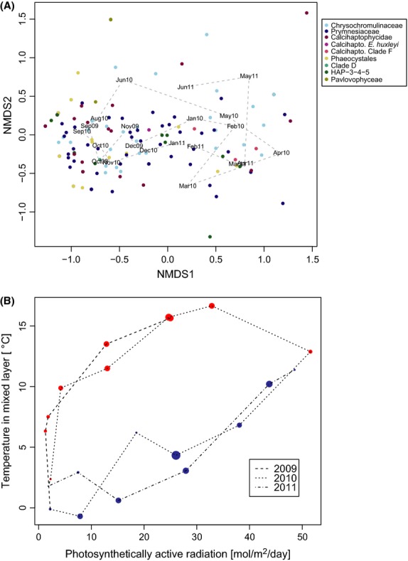
(A) Similarity in OTU composition between the sampling dates, visualized as nonmetric multidimensional scaling (NMDS) ordinations of Jaccard dissimilarities in OTU composition, based on presence–absence data. Stress value: 0.12. The sample scores are indicated by text labels. Species scores, calculated as averages of sample scores and expanded to have equal variance as the site scores, are plotted with colour according to phylogenetic group. (B) Haptophyte community (OTU) composition, represented by the sample scores along the first ordination axis (NMDS 1), in relation to the annual light–temperature cycle. Colour indicates positive (blue) or negative (red) value of the sample score along the NMDS 1 axis; the size of the dots is proportional to the absolute value of the score.

Co-occurrence analysis reveals that the OTUs form clusters largely corresponding to the seasonal distribution (Fig.7). OTUs with more or less overlapping seasonal distributions form one large cluster, with four subnetworks (A–D)—consisting of OTUs found from June to December/January (A), OTUs detected from August to October/November (B), September/October to December (C) and August to February/March (D). In addition, the following clusters were formed: OTUs detected from late autumn (November/December) until May (E), four OTUs only detected in October–November 2010 (F), two OTUs detected all year except in the April samples (G), two OTUs only detected in October 2009 and September 2010 (H), two OTUs co-occurring in June 2010 and September 2009 and 2010 (I) and two OTUs only detected in the September samples, both years (J).

Fig. 7.

Network of co-occurring haptophyte OTUs. Significantly co-occurring OTUs (P < 0.05) are connected with lines. Numbers on the nodes correspond to OTU numbers; colours indicate phylogenetic group. The shaded areas indicate seasonal assemblages of OTUs. (A) OTUs occurring in June–December/January, (B) OTUs detected from August–October/November, (C) September/October–December, (D) August–February/March, (E) OTUs detected from late autumn (November/December), (F) OTUs only detected in October–November 2010, (G) two OTUs detected all year except in the April samples, (H) two OTUs only detected in October 2009 and September 2010, (I) two OTUs co-occurring in June 2010 and September 2009 and 2010 and (J) two OTUs only detected in the September samples, both years.

Plotting sequence similarity against Jaccard distance between OTUs within Prymnesiales did not reveal any relationship between these (Fig. S6, Supporting information); that is, closely related OTUs were neither more nor less likely to co-occur. For the data set as a whole, significant negative co-occurrences were found within and between the major phylogenetic groups (Fig. S7, Supporting information).

Structure of haptophyte diversity

Overall, 80% of the reads were constituted by the 15 most abundant OTUs, which included representatives from all the major groups within class Prymnesiophyceae: Calcihaptophycidae, Phaeocystales, Chrysochromulinaceae and Prymnesiaceae (Fig. S8 and S9A, Supporting information). All the major Prymnesiophyceae groups were also represented among the OTUs that occurred rarely and/or in low proportions (Fig. S9, Supporting information). Seventy OTUs (45% of the OTUs) were each represented by <0.01% of the reads. Most of these matched environmental sequences, but OTUs matching the cultured species Isochrysis galbana (OTU 109), Coccolithus pelagicus ssp. braarudii (OTU 116), Calcidiscus leptoporus (OTU 155) and the freshwater species Chrysochromulina parva (OTU 122) each constituted <0.005% of total reads (table S2 in Egge et al. 2015). Among the most abundant OTUs, we observed considerable variation in proportional read abundance throughout the study period, and only two OTUs, matching C. simplex (OTU 3) and Imantonia sp. (OTU 8), were detected all sampling dates (Figs5 and S5, Supporting information).

The majority (84%) of the OTUs had a closer blast match to an environmental sequence than to a cultured and genetically characterized species (see Egge et al. 2015; Table 2). Of the 15 proportionally most abundant OTUs, 5 had a best match to environmental sequences not linked to a cultured and/or morphologically described species. Among the OTUs occurring in more than 10 samples, 16 of 26 had best match to environmental sequences. Thus, a large part of the proportionally most abundant, and most frequently detected OTUs, represent uncultured and/or not genetically characterized haptophyte species.

Discussion

Haptophyte OTU richness is strongly season dependent

Both OTU richness and composition showed strong temporal variation and were correlated with the annual light and temperature cycle. The correlation between OTU richness and season was strong, with lowest richness in late spring (April–May), and highest in autumn (September–October). Seasonal dynamics and richness of the full haptophyte community have not previously been reported at this level of taxonomic resolution. From previous microscopy surveys from the Skagerrak, it has been shown that certain species of diatoms and dinoflagellates usually dominate in the first and second blooms during spring (Kuylenstierna & Karlson 1994; Kristiansen et al. 1999, 2001), either out-competing other phytoplankton species or overshadowing them. Also within the haptophyte community, our results indicate dominance of a few species in the samples with lowest OTU richness. In 2010, the lowest richness during spring occurred in April and coincided with high proportional abundance of OTU 4, which was also dominating in March 2011. In 2011, the ‘spring minimum richness’ in May coincided with high proportional abundance of P. cordata (OTU 2). Phaeocystis-like cells have also previously been observed to reach maximum abundance in spring in Skagerrak (April 1991; Kuylenstierna & Karlson 1994). Interpolation of the rarefaction curves indicates that the number of reads obtained from these samples was close to saturation (Fig. S3, Supporting information). The low richness was thus due to dominance of these particular OTUs in the haptophyte community, and not a result of insufficient sequencing effort.

Richness increased from June to October–November, in particular within Calcihaptophycidae and Prymnesiales. Light microscopy investigations of noncalcifying haptophyte genera in Nordic waters have usually reported groups of morphologically similar species, or cells identified to order or genus. From such studies, members of Chrysochromulina sensu lato (defined above) and Imantonia (both belonging to Prymnesiales) have been reported as the most abundant groups in June–September/October (Kuylenstierna & Karlson 1994; Dahl & Johannessen 1998; Lekve et al. 2006). Previous electron microscopy investigations of phytoplankton in the Kattegat and Skagerrak have revealed occurrence of c. 30 described and at least 20 not yet described species within Chrysochromulina sensu lato (e.g. Jensen 1998a; Eikrem 1999), and our results confirm that this group is very diverse in outer Oslofjorden. We observed highest richness of Prymnesiales in the summer–autumn months (August–November), with up to 40 co-occurring OTUs belonging to Prymnesiales. According to Estep & MacIntyre (1989), species of Chrysochromulina sensu lato are most often observed in assemblages of >5 species, and Leadbeater (1972) observed 19 species in samples from one station on the Norwegian west coast collected during 12 days in August 1970.

Nutrient concentrations were low during the late summer–autumn months, and under these oligotrophic conditions, mixo- and heterotrophic protists are important components of the plankton community (Kuylenstierna & Karlson 1994). Most of the Prymnesiales OTUs detected in this period did not match sequences from cultured species. Considering recent studies indicating a key role of haptophytes as oceanic bacterivores (Frias-Lopez et al. 2009; Unrein et al. 2014), we speculate that these OTUs may represent K-selected mixo- or heterotrophic species that are competitive under oligotrophic conditions by utilizing organic nutrients, or grazing on prey items. Many of the species easy to cultivate are, however, r-selected, fast growing and autotrophic species that may form blooms and tolerate high inorganic nutrient levels (Brand 1986).

Higher richness and proportional abundance of coccolithophores, in particular E. huxleyi, at higher temperatures in summer–early autumn are consistent with observations by microscopy and general descriptions of phytoplankton succession in Oslofjorden (Hasle & Smayda 1960; Throndsen 1976; Backe-Hansen & Throndsen 2002). Further, there was a significant effect of salinity on OTU richness, where for a given time of year, higher salinity corresponded with higher OTU richness. Higher salinity indicates influence by Atlantic water masses, which may bring oceanic species into the Skagerrak (e.g. Gaarder 1971).

Community composition in relation to environmental factors

Most environmental factors except salinity showed significant seasonal variation, making it difficult to disentangle the effects of individual environmental factors from the general seasonal cycle. However, when we controlled for time of year (i.e. the overall seasonal cycle), residual variation in the factors tested did not have a significant effect on OTU composition. The exception was salinity, which affected the OTU composition of Calcihaptophycidae significantly, but not Prymnesiales. Again, this may be explained by Atlantic water masses bringing different species of coccolithophores into the Skagerrak, as the diversity of coccolithophores is higher in open oceans than in coastal waters in the Atlantic Ocean (e.g. Gaarder 1971 and references therein).

Approximately 30% of the variation in OTU composition could be explained by the yearly light–temperature cycle. The sampling dates grouped as ‘spring’ (January–June) or ‘autumn’ (August–December) communities separated along the first ordination axis. We also found between-year variation in the late winter–late spring communities (January–June), while the late summer–autumn communities (August–December) were quite similar between the 2 years. When only the 15 relatively most abundant OTUs were taken into account, a greater proportion of variation in OTU composition was explained (45%). This suggests that some of the residual variation was caused by species occurring randomly, in low proportions, such as freshwater OTUs (discussed below). The remaining variation may in part be attributed to random abiotic variation, for instance an upwelling event which occurred in winter 2009/2010 (Walday et al. 2012), or to biotic factors like viruses, which are known to be drivers of phytoplankton bloom dynamics at or below species level (e.g. Bratbak et al. 1993; Larsen et al. 2004; Baudoux et al. 2006; Martínez et al. 2012). Abundance of the groups of large viruses did indeed show significant seasonal variation, which suggests that they are also correlated with the phytoplankton seasonal cycle. Several viruses infecting haptophytes have been isolated and genetically characterized (e.g. Suttle & Chan 1995; Sandaa et al. 2001; Johannessen et al. 2014). The genetic diversity of the virus community and seasonal dynamics of virus OTUs in our samples from OF2 has been investigated by 454 pyrosequencing with the major capsid protein gene as marker and will be compared with our results in a following study (S. Gran Stadniczeñko, T. V. Johannessen, E. S. Egge, R. A. Sandaa, B. Edvardsen, unpublished).

‘Background community’ of haptophytes?

Seven OTUs (c. 4% of total OTUs) were detected all year, potentially representing a background community of haptophytes. Among these were OTUs matching Chrysochromulina simplex, found by Jensen (1998a) to be the overall most abundant Chrysochromulina species in a survey of Danish coastal waters, present in all seasons and tolerant to a wide range of temperature and salinity conditions, Imantonia rotunda and Haptolina fragaria/H. ericina/H. hirta, which have all been reported from environments different from Skagerrak such as Australian waters (e.g. LeRoi & Hallegraeff 2004). Further, E. huxleyi, which may form extensive blooms and also is widely distributed, was detected all months except April. Interestingly, among the OTUs detected all year were also OTUs representing deep-branching lineages forming putative new classes of Haptophytes (OTU 30 and 61 nesting within HAP-3 and OTU 15, nesting within HAP-5). To our knowledge, this is the first study reporting on the seasonal distribution of these lineages. Whether the OTUs within these lineages represent unique species or several species that are too closely related to be distinguished by the V4 region is not known. However, that these lineages are detected all year in Skagerrak suggest that they may tolerate a wide range of environmental conditions.

Are seasonal preference and phylogenetic relatedness correlated?

The seasonal assemblages were pluri-phyletic in the sense that we observed members of most clades in most seasons, as can be seen from Figs4 and S5 (Supporting information). Given that a large part of the OTUs showed seasonal preferences, we wanted to investigate whether this was correlated with genetic distance within the order Prymnesiales, which was the most OTU-rich order. If closely related species show similar seasonal preferences, this could indicate that for instance differences in resistance to pathogens (e.g. viruses) or grazer avoidance reduce competition and allow them to co-exist. If the opposite is the case that closely related species tend to not co-occur, this could indicate that they out-compete each other or that they have evolved to occupy different temporal niches (temporal niche partitioning). We did not observe a consistent relationship between genetic distance and co-occurrence (as measured by Jaccard distance) (Fig. S6, Supporting information).

Who are the rare haptophytes?

The rare microbial biosphere and its ecological significance have received increased attention in recent years (Sogin et al. 2006; Caron & Countway 2009; Dawson & Hagen 2009). Considering our data set as a whole, 45% of the OTUs each occurred as <0.01% of the reads, which is considered ‘rare’, according to Logares et al. (2014). The structure of the haptophyte diversity thus seems to reflect that of the total microbial biosphere with a few relatively abundant species/OTUs and several low-abundance ones, as was also found by Bittner et al. (2013). In our study, OTUs occurring seldom and/or in low proportions were found within all the major phylogenetic groups. However, which OTUs occurred in low proportions was highly variable between the sampling dates, as can be seen from Figs5 and S9A (Supporting information). Even the overall most abundant OTU, matching E. huxleyi, occurred as only 0.04% of the reads in February 2010 and was not detected in April 2010 and March–May 2011. Similarly, OTU 7 (5% of total reads), matching P. pouchetii, was not detected from June–October and constituted only 0.2% of the reads in November 2010. Some OTUs occurred in very few samples, but seemed to display a seasonal preference. OTU 91 and 107 (nesting within clade HAP-4) occurred in three samples each: October + November 2009 and November 2010, September 2009 and October + November 2010, respectively. Some of the OTUs occurring seldom were likely allochthonous species brought to the sampling site by dispersion, a mechanism suggested to play a powerful role in shaping microbial communities (Patterson 2009). The coccolithophorid C. leptoporus (OTU 155), detected only in October and November 2010, may have been dispersed by the North Atlantic current. The freshwater species C. parva (OTU 122) and OTUs matching freshwater environmental clones may have been transported from inland lakes via the river Glomma, Norway's longest river which has an outlet in the outer Oslofjorden and is known to influence the hydrological conditions in this area (Walday et al. 2012). Finally, methodological limitations causing bias against certain species should be taken into account when assessing ‘rarity’ of species, for instance, PCR and sequencing bias and retention of colony-forming species in the 45-μm prefiltering step. Forty-six OTUs were only detected at one sampling date (but with >2 reads) throughout the study period. Considering the stringent cleaning of our sequence data set, the number of artefactual OTUs produced by PCR or sequencing error should have been reduced to a minimum, but a few may remain. OTUs occurring in only one sample might be erroneous sequences that slipped through the quality control, but they might also represent species in low abundance or species not detected in other samples due to low relative abundance. For instance, OTU 57, which was 99.7% similar to Chrysochromulina rotalis, only occurred in one sample, but was likely not a result of sequencing error.

Conclusions

The results obtained by HTS methods to investigate seasonal dynamics of haptophytes were, when comparable, consistent with previous microscopy surveys. However, here we obtained taxonomic resolution to species or species-complex level, compared to routine light microscopy surveys where only genus or in most cases order or size category is reported. Further, we were able to observe the seasonal dynamics of OTUs representing putative new orders and classes of haptophytes, for which there is so far no link between 18S rDNA sequence and morphology. We also unveiled the dynamics of described species not previously reported from Skagerrak. The seasonal light–temperature cycle accounted for 29% of the variation in OTU composition in terms of presence–absence. Influence of biotic factors such as virus and between-species competition on the haptophyte temporal dynamics needs to be further investigated. Altogether, these results substantially increase our understanding of the seasonal dynamics and diversity of this ecologically important and, to a large extent, poorly known group of marine protists.

Data accessibility

The raw .sff files from 454 pyrosequencing have been deposited in the Sequence Read Archive with Accession no. PRJEB5541, http://www.ebi.ac.uk/ena/data/view/PRJEB5541.

Environmental data including the flow cytometry counts, the reference alignment, the .tre file of the reference haptophyte tree, a fasta file with the aligned OTUs, the table with taxonomic assignment of each OTU and the read abundance OTU table are deposited in Dryad, doi:10.5061/dryad.b8d21.

Supporting information

Additional supporting information may be found in the online version of this article.

References

- Andersson AF, Riemann L, Bertilsson S. Pyrosequencing reveals contrasting seasonal dynamics of taxa within Baltic Sea bacterioplankton communities. The ISME Journal. 2010;4:171–181. doi: 10.1038/ismej.2009.108. [DOI] [PubMed] [Google Scholar]
- Backe-Hansen P, Throndsen J. Pico- and nanoplankton from the inner Oslofjord, eastern Norway, including description of two new species of Luffisphaera (incerta sedis) Sarsia: North Atlantic Marine Science. 2002;87:55–64. [Google Scholar]
- Baudoux A-C, Nordeloos AAM, Veldhuis MJW, Brussaard CPD. Virally induced mortality of Phaeocystis globosa during two spring blooms in temperate coastal waters. Aquatic Microbial Ecology. 2006;4:207–217. [Google Scholar]
- Bittner L, Gobet A, Audic S, et al. Diversity patterns of uncultured haptophytes unravelled by pyrosequencing in Naples Bay. Molecular Ecology. 2013;22:87–101. doi: 10.1111/mec.12108. [DOI] [PubMed] [Google Scholar]
- Borcard D, Gillet F, Legendre P. Numerical Ecology with r. New York: Springer; 2011. p. 32. [Google Scholar]
- Braarud T, Gaarder K, Nordli O. Seasonal changes in the phytoplankton at various points off the Norwegian West Coast. Norwegian Fishery and Marine Investigations. 1958;XII:1–77. [Google Scholar]
- Brand LE. Nutrition and culture of ultraplankton and picoplankton. In: Platt T, Li W, editors. Photosynthetic picoplankton. Vol. 214. Ottawa, Canada: Canadian Bulletin of Fisheries and Aquatic Sciences Department of Fisheries and Oceans; 1986. pp. 205–233. [Google Scholar]
- Bratbak G, Egge JK, Heldal M. Viral mortality of the marine alga Emiliania huxleyi (Haptophyceae) and termination of algal blooms. Marine Ecology Progress Series. 1993;93:39–48. [Google Scholar]
- Caron DA, Countway PD. Hypotheses on the role of the protistan rare biosphere in a changing world. Aquatic Microbial Ecology. 2009;57:227–238. [Google Scholar]
- Christaki U, Kormas KA, Genitsaris S, et al. Winter-summer succession of unicellular eukaryotes in a meso-eutrophic coastal system. Microbial Ecology. 2014;67:13–23. doi: 10.1007/s00248-013-0290-4. [DOI] [PubMed] [Google Scholar]
- Csardi G, Nepusz T. The igraph software package for complex network research. InterJournal. 2006 Complex Systems:1695. http://igraph.org. [Google Scholar]
- Dahl E, Johannessen T. Temporal and spatial variability of phytoplankton and chlorophyll a : lessons from the south coast of Norway and the Skagerrak. ICES Journal of Marine Sciences. 1998;55:680–687. [Google Scholar]
- Dahl E, Lindahl O, Paasche E, Throndsen J. The Chrysochromulina polylepis bloom in Scandinavian waters during spring 1988. In: Cosper EM, Bricelj VM, Carpenter EJ, editors. Novel Phytoplankton Blooms. Vol. 35. New York: Springer; 1989. pp. 383–405. [Google Scholar]
- Dawson SC, Hagen KD. Mapping the protistan “rare biosphere”. Journal of Biology. 2009;8:105–107. doi: 10.1186/jbiol201. [DOI] [PMC free article] [PubMed] [Google Scholar]
- Dunigan D, Fitzgerald L, Van Etten JL. Phycodnaviruses: A peek at genetic diversity. Virus Research. 2006;117:119–132. doi: 10.1016/j.virusres.2006.01.024. [DOI] [PubMed] [Google Scholar]
- Edvardsen B, Imai I. The ecology of harmful flagellates within Prymnesiophyceae and Raphidophyceae. In: Granéli E, Turner JT, editors. Ecology of Harmful Algae. Vol. 6. Berlin: Springer; 2006. pp. 67–79. [Google Scholar]
- Edvardsen B, Eikrem W, Throndsen J, Sáez AG, Probert I, Medlin LK. Ribosomal DNA phylogenies and a morphological revision provide the basis for a revised taxonomy of the Prymnesiales (Haptophyta) European Journal of Phycology. 2011;46:202–228. [Google Scholar]
- Egge E, Bittner L, Andersen T, Audic S, de Vargas C, Edvardsen B. 454 Pyrosequencing to describe microbial eukaryotic community composition, diversity and relative abundance: a test for marine haptophytes. PLoS ONE. 2013;8:e74371. doi: 10.1371/journal.pone.0074371. [DOI] [PMC free article] [PubMed] [Google Scholar]
- Egge E, Eikrem W, Edvardsen B. Deep-branching novel lineages and high diversity of haptophytes in the Skagerrak (Norway) uncovered by 454 pyrosequencing. The Journal of Eukaryotic Microbiology. 2015;62:121–140. doi: 10.1111/jeu.12157. [DOI] [PMC free article] [PubMed] [Google Scholar]
- Eikrem W. Chrysochromulina throndsenii sp. nov. (Prymnesiophyceae). Description of a new haptophyte flagellate from Norwegian waters. Phycologia. 1996;35:377–380. [Google Scholar]
- Eikrem W. 1999. p. 214. The class Prymnesiophyceae (Haptophyta) in Scandinavian waters. PhD Dissertation, Norway University of Oslo, Oslo.
- Eikrem W, Edvardsen B. Chrysochromulina fragaria sp. nov. (Prymnesiophyceae), a new haptophyte flagellate from Norwegian waters. Phycologia. 1999;38:149–155. [Google Scholar]
- Eikrem W, Throndsen J. The morphology of Chrysochromulina rotalis sp. nov. (Prymnesiophyceae, Haptophyta), isolated from the Skagerrak. Sarsia. 1999;84:445–449. [Google Scholar]
- Estep KW, MacIntyre F. Taxonomy, life cycle, distribution and dasmotrophy of Chrysochromulina: a theory accounting for scales, haptonema, muciferous bodies and toxicity. Marine Ecology Progress Series. 1989;57:11–21. [Google Scholar]
- Frias-Lopez J, Thompson A, Waldbauer J, Chisholm SW. Use of stable isotope-labelled cells to identify active grazers of picocyanobacteria in ocean surface waters. Environmental Microbiology. 2009;11:512–525. doi: 10.1111/j.1462-2920.2008.01793.x. [DOI] [PMC free article] [PubMed] [Google Scholar]
- Gaarder KR. Comments on the distribution of coccolithophorids in the oceans. In: Funnell B, Riedel W, editors. The Micropalaeontology of Oceans. Cambridge: Cambridge University Press; 1971. pp. 97–103. [Google Scholar]
- Gifford SM, Sharma S, Rinta-Kanto J-M, Moran MA. Quantitative analysis of a deeply sequenced marine microbial metatranscriptome. The ISME Journal. 2011;5:461–472. doi: 10.1038/ismej.2010.141. [DOI] [PMC free article] [PubMed] [Google Scholar]
- Gran H. 1930. Skrifter utgitt av det Norske Videnskabs-Akademi i Oslo. 1 Mat.-nat. Klasse.
- Grover JP, Chrzanowski TH. Seasonal dynamics of phytoplankton in two warm temperate reservoirs: association of taxonomic composition with temperature. Journal of Plankton Research. 2005;28:1–17. [Google Scholar]
- Hall TA. bioedit: a user-friendly biological sequence alignment editor and analysis program for Windows 95/98/NT. Nucleic Acids Symposium Series. 1999;41:95–98. [Google Scholar]
- Hartmann M, Grob C, Tarran GA, et al. Mixotrophic basis of Atlantic oligotrophic ecosystems. Proceedings of the National Academy of Sciences USA. 2012;109:5756–5760. doi: 10.1073/pnas.1118179109. [DOI] [PMC free article] [PubMed] [Google Scholar]
- Hasle GR, Smayda TJ. The annual phytoplankton cycle at Drøbak, Oslofjord. Nytt Magasin for Botanikk. 1960;8:53–75. [Google Scholar]
- Hurlbert SH. The nonconcept of species diversity: a critique and alternative parameters. Ecology. 1971;52:577–586. doi: 10.2307/1934145. [DOI] [PubMed] [Google Scholar]
- Jardillier L, Zubkov MV, Pearman J, Scanlan DJ. Significant CO2 fixation by small prymnesiophytes in the subtropical and tropical Northeast Atlantic Ocean. The ISME Journal. 2010;4:1180–1192. doi: 10.1038/ismej.2010.36. [DOI] [PubMed] [Google Scholar]
- Jensen MØ. 1998a. p. 200. The genus Chrysochromulina (Prymnesiophyceae) in Scandinavian coastal waters—diversity, abundance and ecology. PhD Dissertation, University of Copenhagen, Copenhagen, Denmark.
- Jensen MØ. A new method for fixation of unmineralized haptophytes for TEM (whole mount) investigations. Journal of Phycology. 1998b;34:558–560. [Google Scholar]
- Johannessen TV, Bratbak G, Larsen A, et al. Characterisation of three novel giant viruses reveals huge diversity among viruses infecting Prymnesiales (Haptophyta) Virology. 2014;476:180–188. doi: 10.1016/j.virol.2014.12.014. [DOI] [PubMed] [Google Scholar]
- Jordan R, Chamberlain A. Biodiversity among haptophyte algae. Biodiversity and Conservation. 1997;6:131–152. [Google Scholar]
- Katoh K, Frith MC. Adding unaligned sequences into an existing alignment using mafft and LAST. Bioinformatics. 2012;28:3144–3146. doi: 10.1093/bioinformatics/bts578. [DOI] [PMC free article] [PubMed] [Google Scholar]
- Kristiansen S, Farbrot T, Naustvoll L-J. Fate of a spring bloom in the Oslofjord. In: Heiskanen AS, Lundsgaard C, Reigstadt M, Oll K, Floderus S, editors. Sedimentation and Recycling in Aquatic Ecosystems—the Impact of Pelagic Processes and Planktonic Food Web Structure. Helsinki: Finnish Environment Institute; 1999. pp. 21–30. [Google Scholar]
- Kristiansen S, Farbrot T, Naustvoll L-J. Spring bloom nutrient dynamics in the Oslofjord. Marine Ecology Progress Series. 2001;219:41–49. [Google Scholar]
- Kuylenstierna M, Karlson B. Seasonality and composition of pico- and nanoplanktonic cyanobacteria and protists in the Skagerrak. Botanica Marina. 1994;37:17–34. [Google Scholar]
- Larsen A, Castberg T, Sandaa R-A, et al. Population dynamics and diversity of phytoplankton, bacteria and viruses in a seawater enclosure. Marine Ecology Progress Series. 2001;221:47–57. [Google Scholar]
- Larsen A, Flaten GAF, Sandaa R-A, et al. Spring phytoplankton bloom dynamics in Norwegian coastal waters: microbial community succession and diversity. Limnology and Oceanography. 2004;49:180–190. [Google Scholar]
- Leadbeater BSC. Fine structural observations on six new species of Chrysochromulina (Haptophyceae) from Norway. Sarsia. 1972;49:65–80. [Google Scholar]
- Lekve K, Bagøien E, Dahl E, Edvardsen B, Skogen M, Stenseth NC. Environmental forcing as a main determinant of bloom dynamics of the Chrysochromulina algae. Proceedings of the Royal Society B: Biological Sciences. 2006;273:3047–3055. doi: 10.1098/rspb.2006.3656. [DOI] [PMC free article] [PubMed] [Google Scholar]
- Lentendu G, Wubet T, Chatzinotas A, Wilhelm C, Buscot F, Schlegel M. Effects of long-term differential fertilization on eukaryotic microbial communities in an arable soil: a multiple barcoding approach. Molecular Ecology. 2014;23:3341–3355. doi: 10.1111/mec.12819. [DOI] [PubMed] [Google Scholar]
- LeRoi JM, Hallegraeff GM. Scale-bearing nanoflagellates from southern Tasmanian coastal waters, Australia. I. Species of the genus Chrysochromulina (Haptophyta) Botanica Marina. 2004;47:73–102. [Google Scholar]
- Logares R, Audic S, Bass D, et al. Patterns of rare and abundant marine microbial Eukaryotes. Current Biology. 2014;24:813–821. doi: 10.1016/j.cub.2014.02.050. [DOI] [PubMed] [Google Scholar]
- Majaneva M, Rintala J-M, Piisilä M, Fewer DP, Blomster J. Comparison of wintertime eukaryotic community from sea ice and open water in the Baltic Sea, based on sequencing of the 18S rRNA gene. Polar Biology. 2011;35:875–889. [Google Scholar]
- Marie D, Brussaard CP, Thyrhaug R, Bratbak G, Vaulot D. Enumeration of marine viruses in culture and natural samples by flow cytometry. Applied Environmental Microbiology. 1999;65:45–52. doi: 10.1128/aem.65.1.45-52.1999. [DOI] [PMC free article] [PubMed] [Google Scholar]
- Martínez JM, Schroeder DC, Wilson WH. Dynamics and genotypic composition of Emiliania huxleyi and their co-occurring viruses during a coccolithophore bloom in the North Sea. FEMS Microbiology Ecology. 2012;81:315–323. doi: 10.1111/j.1574-6941.2012.01349.x. [DOI] [PubMed] [Google Scholar]
- McMurdie PJ, Holmes S. phyloseq: an r package for reproducible interactive analysis and graphics of microbiome census data. PLoS ONE. 2013;8:e61217. doi: 10.1371/journal.pone.0061217. [DOI] [PMC free article] [PubMed] [Google Scholar]
- Oksanen J. 2011. Multivariate Analysis of Ecological Communities in r: vegan tutorial. URL: http://cc.oulu.fi/~jarioksa/opetus/metodi/vegantutor.pdf.
- Oksanen J, Blanchet G, Kindt R, et al. 2012. vegan: Community Ecology Package. URL: http://cran.r-project.org/package=vegan.
- Paasche E. The spring development of phytoplankton in the Atlantic Waters of the Norwegian Sea in 1958. International Council for the exploration of the sea. Plankton Committee. 1961;52:1–5. [Google Scholar]
- Patterson DJ. Ecology. Seeing the big picture on microbe distribution. Science. 2009;325:1506–1507. doi: 10.1126/science.1179690. [DOI] [PubMed] [Google Scholar]
- Paul JH, Cazares L, Thurmond J. Amplification of the rbcL gene from dissolved and particulate DNA from aquatic environments. Applied Environmental Microbiology. 1990;56:1963–1966. doi: 10.1128/aem.56.6.1963-1966.1990. [DOI] [PMC free article] [PubMed] [Google Scholar]
- Quince C, Lanzén A, Davenport RJ, Turnbaugh PJ. Removing noise from pyrosequenced amplicons. BMC Bioinformatics. 2011;12:38. doi: 10.1186/1471-2105-12-38. [DOI] [PMC free article] [PubMed] [Google Scholar]
- R Development Core Team. Vienna, Austria: R Foundation for Statistical Computing; 2013. rA Language and Environment for Statistical Computing. URL http://www.R-project.org/ [Google Scholar]
- Rosenberg R, Lindahl O, Blanck H. Silent spring in the sea. Ambio. 1988;17:289–290. [Google Scholar]
- Sandaa RA, Heldal M, Castberg T, Thyrhaug R, Bratbak G. Isolation and characterization of two viruses with large genome size infecting Chrysochromulina ericina (Prymnesiophyceae) and Pyramimonas orientalis (Prasinophyceae) Virology. 2001;290:272–280. doi: 10.1006/viro.2001.1161. [DOI] [PubMed] [Google Scholar]
- Sogin ML, Morrison HG, Huber JA, et al. Microbial diversity in the deep sea and the underexplored “rare biosphere”. Proceedings of the National Academy of Sciences USA. 2006;103:12115–12120. doi: 10.1073/pnas.0605127103. [DOI] [PMC free article] [PubMed] [Google Scholar]
- Sørensen N, Daugbjerg N, Richardson K. Choice of pore size can introduce artefacts when filtering picoeukaryotes for molecular biodiversity studies. Microbial Ecology. 2013;65:964–968. doi: 10.1007/s00248-012-0174-z. [DOI] [PubMed] [Google Scholar]
- Stamatakis A. raxml-VI-HPC: maximum likelihood-based phylogenetic analyses with thousands of taxa and mixed models. Bioinformatics. 2006;22:2688–2690. doi: 10.1093/bioinformatics/btl446. [DOI] [PubMed] [Google Scholar]
- Stoeck T, Bass D, Nebel M, et al. Multiple marker parallel tag environmental DNA sequencing reveals a highly complex eukaryotic community in marine anoxic water. Molecular Ecology. 2010;19:21–31. doi: 10.1111/j.1365-294X.2009.04480.x. [DOI] [PubMed] [Google Scholar]
- Strickland J, Parsons T. A practical handbook of seawater analysis. Bulletin of Fisheries Research Board of Canada. 1968;167:1–310. [Google Scholar]
- Suttle C, Chan A. Viruses infecting the marine Prymnesiophyte Chrysochromulina spp.: isolation, preliminary characterization and natural abundance. Marine Ecology Progress Series. 1995;118:275–282. [Google Scholar]
- Thomsen HA, Buck KR, Chavez FP. Haptophytes as components of marine phytoplankton. In: Green JC, Leadbeater BSC, editors. The Haptophyte Algae. 1st edn. Vol. 10. Oxford: Clarendon Press; 1994. pp. 187–208. [Google Scholar]
- Throndsen J. Ultra- and nannoplankton flagellates in the Oslofjord, Norway. Blyttia. 1976;34:237–246. [Google Scholar]
- Tillmann U. Kill and eat your predator: a winning strategy of the planktonic flagellate Prymnesium parvum. Aquatic Microbial Ecology. 2003;32:73–84. [Google Scholar]
- Ulrich W. 2008. Pairs—A FORTRAN Program for Studying Pairwise Species Associations in Ecological Matrices. URL http://www.keib.umk.pl/pairs/
- Unrein F, Gasol JM, Not F, Forn I, Massana R. Mixotrophic haptophytes are key bacterial grazers in oligotrophic coastal waters. The ISME Journal. 2014;8:164–176. doi: 10.1038/ismej.2013.132. [DOI] [PMC free article] [PubMed] [Google Scholar]
- Walday M, Gitmark J, Naustvoll LJ, Norling K, Selvik JR, Sørensen K. 2011. Monitoring of the outer Oslofjord 2010. Norway Norwegian Institute of Water Research, Oslo.
- Walday M, Gitmark J, Naustvoll LJ, Norling K, Selvik JR, Sørensen K. Monitoring of the Outer Oslofjord 2007–2011. 5-Year Report. 2012. Oslo, Norway Norwegian Institute of Water Research.
Associated Data
This section collects any data citations, data availability statements, or supplementary materials included in this article.
Supplementary Materials
Table S1 Sampling dates, number of clean Haptophyta reads in each sample, and depth of mixed layer.
Table S2 Seasonal variation in environmental variables and FCM counts from Skagerrak, assessed by fit to trigonometric functions.
Fig. S1 Comparison of NMDS ordination of Jaccard dissimilarities between the sampling dates, based on presence-absence-transformed (A) non-subsampled and (B) dataset subsampled to 5553 reads.
Fig. S2 Profiles and contour plots of physical and chemical parameters each sampling date. (A) Log-transformed irradiance profiles. Secchi depth is indicated by pink line. (B–E) Contour plots of (B) temperature, (C) salinity, (D) density and (E) fluorescence from 1 to 40 m depth.
Fig. S3 Rarefaction curves for each sample.
Fig. S4 OTU richness as a function of time-of-year (season).
Fig. S5 Monthly detection patterns of haptophyte OTUs when the two sampling years are considered together. OTUs only occurring in one sample are omitted.
Fig. S6 Relationship between sequence similarity and Jaccard distance between the OTUs nesting within Prymnesiales.
Fig. S7 Significant negative co-occurrences between haptophyte OTUs.
Fig. S8 (A) Rank-abundance plot, (B) Accumulation curve of the total dataset.
Fig. S9 Rank-abundance of OTUs based on (A) Boxplots of proportion of reads in each sample throughout the sampling period (normalised to even sampling depth) (B) Number of sampling dates the OTUs were detected.
Data Availability Statement