Titian: Data Provenance Support in Spark

Abstract

Debugging data processing logic in Data-Intensive Scalable Computing (DISC) systems is a difficult and time consuming effort. Today’s DISC systems offer very little tooling for debugging programs, and as a result programmers spend countless hours collecting evidence (e.g., from log files) and performing trial and error debugging. To aid this effort, we built Titian, a library that enables data provenance—tracking data through transformations—in Apache Spark. Data scientists using the Titian Spark extension will be able to quickly identify the input data at the root cause of a potential bug or outlier result. Titian is built directly into the Spark platform and offers data provenance support at interactive speeds—orders-of-magnitude faster than alternative solutions—while minimally impacting Spark job performance; observed overheads for capturing data lineage rarely exceed 30% above the baseline job execution time.

1. INTRODUCTION

Data-Intensive Scalable Computing (DISC) systems, like Apache Hadoop [1] and Apache Spark [3], are being used to analyze massive quantities of data. These DISC systems expose a programming model for authoring data processing logic, which is compiled into a Directed Acyclic Graph (DAG) of data-parallel operators. The root DAG operators consume data from an input source (e.g., GFS [13], or HDFS), while downstream operators consume the intermediate outputs from DAG predecessors. Scaling to large datasets is handled by partitioning the data and assigning tasks that execute the operator logic on each partition.

Debugging data processing logic in DISC environments can be daunting. A recurring debugging pattern is to identify the subset of data leading to failures, crashes, and exceptions. Another desirable pattern is trial-and-error debugging, where developers selectively replay a portion of their data processing steps on a subset of intermediate data leading to outlier or erroneous results. These features motivate the need for capturing data provenance (also referred to as data lineage) and supporting appropriate provenance query capabilities in DISC systems. Such support would enable the identification of the input data leading to a failure, crash, exception, or outlier results. Our goal is to provide interactive data provenance support that integrates with the DISC programming model and enables the above debugging scenarios.

Current approaches supporting data lineage in DISC systems (specifically RAMP [18] and Newt [21]) do not meet our goals due to the following limitations: (1) they use external storage such as a sharded DBMS or distributed file systems (e.g., HDFS) to retain lineage information; (2) data provenance queries are supported in a separate programming interface; (3) they provide very little support for viewing intermediate data or replaying (possibly alternative) data processing steps on intermediate data. These limitations prevent support for interactive debugging sessions. Moreover, we show that these approaches do not operate well at scale because they store the data lineage externally.

In this paper we introduce Titian, a library that enables interactive data provenance in Apache Spark. Titian integrates with the Spark programming interface, which is based on a Resilient Distributed Dataset (RDD) abstraction defining a set of transformations and actions that process datasets. The data from a particular sequence of transformations, leading to an RDD, can be cached in memory. Spark maintains the program transformation lineage so that it can reconstruct lost RDD partitions in the case of a failure.

Titian enhances the RDD abstraction with fine-grained data provenance capabilities. From any given RDD, a Spark programmer can obtain a LineageRDD reference, which enables data tracing functionality i.e., the ability to transition backward (or forward) in the Spark program dataflow. From a given LineageRDD reference, corresponding to a position in the program’s execution, any native RDD transformation can be called, returning a new RDD that will execute the transformation on the subset of data referenced by the LineageRDD. As we will show, this facilitates the ability to trace backward (or forward) in the dataflow, and from there execute a new series of native RDD transformations on the reference data. The tracing support provided by LineageRDD integrates with Spark’s internal batch operators and fault-tolerance mechanisms. As a result, Titian can be used in a Spark terminal session, providing interactive data provenance support along with native Spark ad-hoc queries.

To summerize, Titian offers the following contributions:

• A data lineage capture and query support system in Apache Spark.

• Lineage capturing design that minimizes the overhead on the target Spark program—most experiments exhibit an overhead of less than 30%.

• We show that our approach scales to large datasets with less overhead compared to prior work [18, 21].

• Interactive data provenance query support that extends the familiar Spark RDD programming model.

• A evaluation of Titian that includes a variety of design alternatives for capturing and tracing data lineage.

The remainder of the paper is organized as follows. Section 2 contains a brief overview of Spark, and discusses our experience with using alternative data provenance libraries with Spark. Section 3 defines the Titian programming interface. Section 4 describes Titian provenance capturing model, and its implementation. The experimental evaluation of Titian is presented in Section 5. Related work is covered in Section 6. Section 7 concludes with future directions in the DISC debugging space.

2. BACKGROUND

This section provides a brief background on Apache Spark, which we have instrumented with data provenance capabilities (Section 3). We also review RAMP [18] and Newt [21], which are toolkits for capturing data lineage and supporting offline data provenance analysis of DISC programs. Our initial work in this area leveraged these two toolkits for data provenance support in Spark. During this exercise, we encountered a number of issues, including scalability (the sheer amount of lineage data that could be supported in capturing and tracing), job overhead (the per-job slowdown incurred from lineage capture), and usability (both RAMP and Newt come with limited support for data provenance queries). RAMP and Newt operate externally to the target DISC system, making them more general i.e., able to instrument with Hyracks [9], Hadoop [1], Spark [27], for example. However, this prevents a unified programming environment, in which both data analysis and data provenance queries can operate in concert. Moreover, Spark programmers are accustom to an interactive development environment, which we want to support.

2.1 Apache Spark

Spark is a DISC system that exposes a programming model based on Resilient Distributed Datasets (RDDs) [27]. The RDD abstraction provides transformations (e.g., map, reduce, filter, group-by, join, etc.) and actions (e.g., count, collect) that operate on datasets partitioned over a cluster of nodes. A typical Spark program executes a series of transformations ending with an action that returns a result value (e.g., the record count of an RDD, a collected list of records referenced by the RDD) to the Spark “driver” program, which could then trigger another series of RDD transformations. The RDD programming interface can support these data analysis transformations and actions through an interactive terminal, which comes packaged with Spark.

Spark driver programs run at a central location and operate on RDDs through references. A driver program could be a user operating through the Spark terminal, or it could be a standalone Scala program. In either case, RDD references lazily evaluate transformations by returning a new RDD reference that is specific to the transformation operation on the target input RDD(s). Actions trigger the evaluation of an RDD reference, and all RDD transformations leading up to it. Internally, Spark translates a series of RDD transformations into a DAG of stages, where each stage contains some sub-series of transformations until a shuffle step is required (i.e., data must be re-partitioned). The Spark scheduler is responsible for executing each stage in topological order, with tasks that perform the work of a stage on each input partition. Each stage is fully executed before downstream dependent stages are scheduled i.e., Spark batch executes the stage DAG. The final output stage evaluates the action that triggered the execution. The action result values are collected from each task and returned to the driver program, which can initiate another series of transformations ending with an action. Next, we illustrate the Spark programming model with a running example used throughout the paper.

Running example

Assume we have a large log file stored in a distributed file system such as HDFS. The Spark program in Figure 1 selects all lines containing errors, counts the number of error occurrences grouped by the error code, and returns a report containing the description of each error, together with its count.

Figure 1.

Running example: log analysis

The first line loads the content of the log file from HDFS and assigns the result RDD to the lines reference. It then applies a filter transformation on lines and assigns the result RDD to the errors reference, which retains lines with errors.¹ The transformations in lines 3 and 4 are used to (1) extract an error code, and (2) pair each error code with the value one i.e., the initial error code count. The reduceByKey transformation sums up the counts for each error code which is then mapped into a textual error description referenced by reports in line 6.² The collect action triggers the evaluation of the reports RDD reference, and all transformations leading up to it. The collect action result is returned to the driver program, which prints each result record.

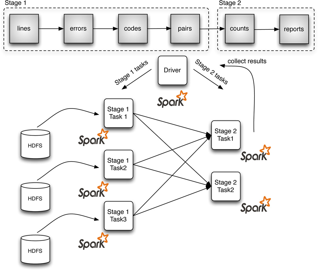
Figures 2 schematically represents a toy Spark cluster executing this example on a log file stored in three HDFS partitions. The top of the figure illustrates the stage DAG internally constructed by Spark. The first stage contains the lines, errors, codes, and pairs reference transformations. The second stage contains (1) the counts reference produced by the reduceByKey transformation, which groups the records by error code in a shuffle step, and (2) the final map transformation that generates the reports reference.

Figure 2.

Example Spark cluster running a job instance executing tasks that run the stage logic on input partitions.

The collect action triggers the execution of these two stages in the Spark driver, which is responsible for instantiating the tasks that execute the stage DAG. In the specific case of Figure 2, three tasks are used to execute Stage 1 on the input HDFS partitions. The output of Stage 1 is shuffled into two partitions of records grouped by error code, which is also naturally the partitioning key. Spark then schedules a task on each of the two shuffled partitions to execute the reduceByKey transformation (i.e., sum) in Stage 2, ending with the final map transformation, followed by the collect action result, which is sent back to the driver.

2.2 Data Provenance in DISC

RAMP [18] and Newt [21] address the problem of supporting data provenance in DISC systems through an external, generic library. For example, RAMP instruments Hadoop with “agents” that wrap the user provided map and reduce functions with lineage capture capabilities. RAMP agents store data lineage in HDFS, where toolkits like Hive [25] and Pig [24] can be leveraged for data provenance queries. Newt is a system for capturing data lineage specifically designed to “discover and resolve computational errors.” Like RAMP, Newt also injects agents into the dataflow to capture and store data lineage; in this case, in a cluster of MySQL instances running along side the target system e.g., the Newt paper describes data provenance support in Hadoop and Hyracks [9]. Data provenance queries are supported in Newt by directly querying (in SQL) the data lineage that it stores in the MySQL cluster.

Tracing through the evolution of record data in a DISC dataflow is a common data provenance query. Newt also references support for replaying the program execution on a subset of input data that generated a given result e.g., an outlier or erroneous value. Naturally, this first requires the ability to trace to the input data leading to a final result. We use the term trace to refer to the process of identifying the input data that produced a given output data record set. In the context of Spark, this means associating each output record of a transformation (or stage, in Titian’s case) with the corresponding input record. Tracing can then be supported by recursing through these input to output record associations to a desired point in the dataflow.

2.3 Newt and RAMP Instrumentation

Our first attempt at supporting data provenance in Spark leveraged Newt to capture data lineage at stage boundaries. However, we ran into some issues. To leverage Newt, we first had to establish and manage a MySQL cluster along side our Spark cluster. Second, we ran into scalability issues: as the size of data lineage (record associations) grew large, the Spark job response time increased by orders-of-magnitude. Third, tracing support was limited: for instance, to perform a trace in Newt we were required to submit SQL queries records with corresponding input records, in an iterative loop. This was done outside of the Spark interactive terminal session in a Python script. Lastly, both Newt and RAMP do not store the referenced raw data³, preventing us from viewing any intermediate data leading to a particular output result. It was also unclear to us, based on this issue, how “replay” on intermediate data was supported in Newt.

Based on the reference Newt documentation, our instrumentation wraps Spark stages with Newt agents that capture data lineage. Newt agents create unique identifiers for individual data records, and maintain references that associated output record identifiers with the relevant input record identifiers. The identifiers and associations form the data lineage, which Newt agents store in MySQL tables.

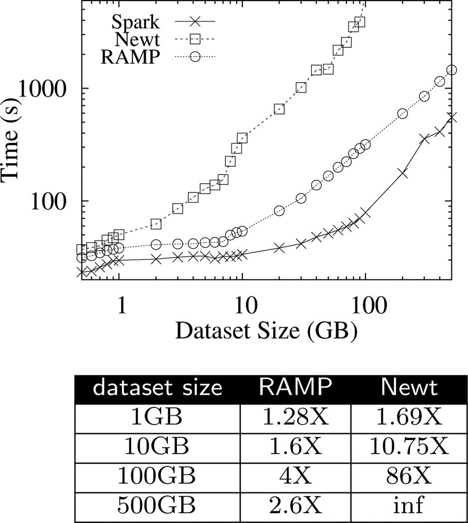
Figure 3 gives a quantitative assessment of the additional time needed to execute a word count job when capturing lineage with Newt. The results also include a version of the RAMP design that we built in the Titian framework. For this experiment, only RAMP is able to complete the workload in all cases, incurring a fairly reasonable amount of overhead i.e., RAMP is on average 2.3× the Spark execution time. However, the overhead observed in Newt is considerably worse (up to 86× the Spark run time), preventing the ability to operate at 500GB. Simply put, MySQL could not sustain the data lineage throughput observed in this job. A more detailed description is available in Section 5.

Figure 3.

Run time of Newt and RAMP data lineage capture in a Spark word count job. The table summarizes the plot results at four dataset sizes, and indicates the run time as a multiplier of the native Spark job execution time.

3. DATA PROVENANCE IN SPARK

Titian is a library that supports data provenance in Spark through a simple LineageRDD application programming interface, which extends the familiar RDD abstraction with tracing capabilities. This section describes the extensions provided by LineageRDD along with some example provenance queries that use those extensions in concert with native RDD transformations (e.g., filter). Since our design integrates with the Spark programming model and runtime, Titian extensions can be used in interactive Spark sessions for exploratory data analysis.

Titian extends the native Spark RDD interface with a method (getLineage) that returns a LineageRDD, representing the starting point of the trace. From there, LineageRDD supports methods that travel through the transformation dataflow at stage boundaries.

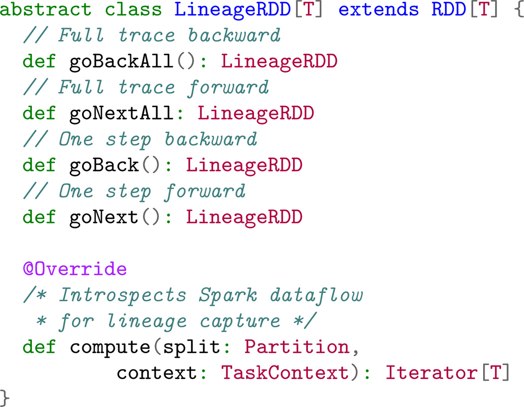
Figure 4 lists the transformations that LineageRDD supports. The goBackAll and goNextAll methods can be used to compute the full trace backward and forward respectively. That is, given some result record(s), goBackAll returns all initial input records that contributed—through the transformation series leading to—the result record(s); goNextAll returns all the final result records that a starting input record(s) contributed to in a transformation series. A single step backward or forward is supported by the goBack and goNext respectively.

Figure 4.

LineageRDD methods for traversing through the data lineage in both backward and forward directions. The native Spark compute method is used to plug a LineageRDD instance into the Spark dataflow (described in Section 4).

These tracing methods behave similarly to a native RDD transformation, in that they return a new LineageRDD corresponding to the traced point, without actually evaluating the trace. The actual tracing occurs when a native Spark RDD action, such as count or collect, is called; similar to the lazy evaluation semantics of Spark. For instance, if a user wants to trace back to an intermediate point and view the data, then she could execute a series of goBack transformations followed by a native Spark collect action. The compute method, defined in the native RDD class, is used to introspect the stage dataflow for data lineage capture.

Since LineageRDD extends the native Spark RDD interface, it also includes all native transformations. Calling a native transformation on a LineageRDD returns a new native RDD that references the (raw) data at the traced point and the desired transformation that will process it. This mode of operation forms the basis of our replay support. Users can trace back from a given RDD to an intermediate point, and then leverage native RDD transformations to reprocess the referenced data. We highlight these Titian extensions in the example Spark program below.

Example 1: Backward Tracing

Titian is enabled by wrapping the native SparkContext (sc in line 1 of Figure 1) with a LineageContext. Figure 5 shows a code fragment that takes the result of our running example in Figure 1 and selects the most frequent error (via a native Spark sortBy and take operations), then traces back to the input lines containing such errors and prints them.

Figure 5.

Input lines with the most frequent error

Next, we describe an example of forward tracing from input records to records in the final result that the input records influenced.

Example 2: Forward Tracing

Here, we are interested in the error codes generated from the network sub-system, indicated in the log by a “NETWORK” tag.

Again, assume the program in Figure 1 has finished executing. Figure 6 selects log entries related to the network layer (line 1), and then performs a goNextAll (line 3) on the corresponding LineageRDD reference (obtained in line 2). Finally, the relevant output records containing the error description and count are printed (line 4).

Figure 6.

Network-related error codes

Provenance queries and actual computation can be interleaved in a natural way. This unlocks the possibility to interactively explore and debug Spark programs.

Example 3: Selective Replay

Assume that after computing the error counts, we traced backward and notice that many errors were generated by the “Guest” user. We are then interested in seeing the errors distribution without the ones caused by “Guest.” This can be specified by tracing back to the input, filtering out “Guest”, and then re-executing the computation, as shown in Figure 7. This is made possible because native RDD transformations can be called from a LineageRDD. Supporting this requires Titian to automatically retrieve the raw data referenced by the lineage and applying the native (replay) transformations to it.

Figure 7.

Error codes without “Guest”

4. TITIAN INTERNAL LIBRARY

Titian is our extension to Spark that enables interactive data provenance on RDD transformations. This section describes the agents used to introspect Spark RDD transformations to capture and store data lineage. We also discuss how we leverage native RDD transformations to support traces through the data provenance via the LineageRDD interface.

4.1 Overview

Similar to other approaches [21, 18, 23], Titian uses agents to introspect the Spark’s stage DAG to capture data lineage. The primary responsibility of these agents are to (1) generate unique identifiers for each new record, and (2) associate output records of a given operation (i.e., stage, shuffle step) with relevant input records.

From a logical perspective, Titian generates new records in three places:

1. Input: Data imported from some external source e.g., HDFS, Java Collection, etc.

2. Stage: The output of a stage executed by a task.

3. Aggregate: In an aggregation operation i.e., combiner, group-by, reduce, and join.

Recall that each stage executes a series of RDD transformations until a shuffle step is required. Stage input records could come from an external data source (e.g., HDFS) or from the result of a shuffle step. Input agents generate and attach a unique identifier to each input record. Aggregate agents generate unique identifiers for each output record, and relate an output record to all input records in the aggregation operation i.e., combiner, reduce, group-by, and join. A Spark stage processes a single input record at a time, and produces zero or more output records. Stage agents attach a unique identifier to each output record of a stage and associates it with the relevant input record identifier.

Associations are stored in a table on the local Spark storage layer (i.e., BlockManager). The schema of the table defines two columns containing the (1) input record identifiers, and (2) output record identifiers. Tracing occurs by recursively joining the tables.

Remark

Titian captures data lineage at the stage boundaries, but this does not prevent tracing to an RDD transformation within a stage. Such a feature could be supported by tracing back to the stage input and re-running the stage transformations, on the referenced intermediate data, up to the RDD transformation of interest. Alternatively, we could surface an API that would allow the user to mark RDD transformation as a desirable trace point. Stage agents could then be injected at these markers.

4.2 Capturing Agents

Titian instruments a Spark dataflow with agents on the driver i.e., where the main program executes. Recall that when the main program encounters an action, Spark translates the series of transformations, leading to the action, into a DAG of stages. The LineageContext hijacks this step and supplements the stage DAG with capture agents, before it is submitted to the task scheduler for execution.

Table 1 lists the agents that Titian uses at each capture point i.e., Input, Stage, and Aggregate. We have defined two input agents. Both assign identifiers to records emitted from a data source. The identifier should be meaningful to the given data source. For instance, the HadoopLineageRDD assigns an identifier that indicates the HDFS partition and record position (e.g., line offset) within the partition. The ParallelLineageRDD assigns identifiers to records based on its location in a Java Collection Object e.g., java.util.ArrayList.

Table 1.

Lineage capturing points and agents.

Capture Point	LineageRDD Agent
Input	HadoopLineageRDD
	ParallelLineageRDD
Stage	StageLineageRDD
Aggregate	ReducerLineageRDD
	JoinLineageRDD
	CombinerLineageRDD

A Spark stage consists of a series of transformations that process a single record at a time, and emit zero or more records. At the stage output, Titian will inject a CombinerLineageRDD when a combiner operation is present, or a StageLineageRDD when a combiner is not present. Both agents are responsible for relating output to input record(s). In the case of a StageLineageRDD, for each output record produced, it generates an identifier and associates that identifier with the (single) input record identifier. A combiner pre-aggregates one or more input records, and generates a new combined output record. For this case, Titian injects a CombinerLineageRDD, which is responsible for generating an identifier for the combined output record, and associating that identifier with the identifiers of all related inputs.

The other two aggregate capture agents introspect the Spark dataflow in the shuffle step used to execute reduce, group-by, and join transformations. Similar to the combiner, these transformations take one or more input records and produce a new output record; unlike the combiner, join operations could produce more than one output record. The reduce and group-by transformations operate on a single dataset (i.e., RDD), while join operates on multiple datasets. The ReducerLineageRDD handles the reduce and group-by aggregates, while JoinLineageRDD handles the join operation. The ReducerLineageRDD associates an output record identifier with all input record identifiers that form the aggregate group. While JoinLineageRDD associates an output (join) record identifier with the record identifiers on each side of the join inputs.

Remark

Joins in Spark behave similar to Pig [24] and Hive [25]: records that satisfy the join are grouped together based on the “join key.” For this reason, we have categorized JoinLineageRDD as an aggregate, even though this is not the case logically.

Example 4: Dataow Instrumentation

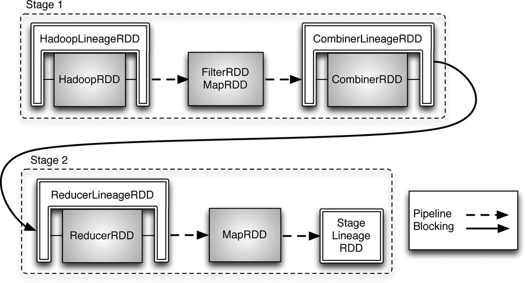
Returning to our running example, Figure 8 shows the workflow after the instrumentation of capture agents. The Spark stage DAG consists of two stages separated by the reduceByKey transformation. The arrows indicate how records are passed through the dataflow. A dashed-arrow means that records are pipelined (i.e., processed one at a time) by RDD transformations e.g., FilterRDD, and MapRDD in stage 1. A solidarrow indicates a blocking boundary, where input records are first materialized (i.e., drained) before the given operation begins its processing step e.g., Spark’s combiner materializes all input records into an internal hash-table, which is then used to combine records in the same hash bucket.

Figure 8.

Job workflow after adding the lineage capture points

The transformed stage DAG includes (1) a Hadoop LineageRDD agent that introspects Spark’s native Hadoop RDD and assigns an identifier to each record. It then associates the record identifier to the record position in the HDFS partition; (2) a CombinerLineageRDD assigns an identifier to each record emitted from the combiner (pre-aggregation) operation, and associates it with the (combiner input) record identifiers assigned by HadoopLineageRDD; (3) a ReduceLineageRDD that assigns an identifier to each reduceByKey output record, and associates it with each record identifier in the input group aggregate; and (4) a StageLineageRDD that assigns an identifier to each stage record output and relates that identifier back to the respective input (reducer) record identifier.

4.3 Lineage Capturing

Data lineage capture begins in the agent compute method implementation, defined in the native Spark RDD class, and overridden in the LineageRDD class. The arguments to this method (Figure 4) include the input partition—containing the stage input records—and a task context. The return value is an iterator over the resulting output records. Each agent’s compute method passes the partition and task context arguments to its parent RDD(s) compute method, and wraps the returned parent iterator(s) in its own iterator module, which it returns to the caller.

Input to Output Identifier Propagation

Parent (upstream) agents propagate record identifiers to a child (downstream) agent. Two configurations are possible: (1) propagation inside a single stage, and (2) propagation between consecutive stages. In the former case, Titian exploits the fact that stage records are pipelined one at a time through the stage transformations. Before sending a record to the stage transformations, the agent at the input to a stage stores the single input record identifier in the task context. The agent at the stage transformation output associates output record identifiers with the input record identifier stored in the task context. Between consecutive stages, Titian attaches (i.e., piggybacks) the record identifier on each outgoing (shuffled) record. On the other side of the shuffle step, the piggybacked record identifier is grouped with the other record identifiers containing the same key (from the actual record). Each group is assigned a new identifier, which will be associated with all record identifiers in the group. Next, we describe the implementation of each agent’s iterator.

HadoopLineageRDD parent RDD is a native Hadoop RDD. In its iterator, it assigns an identifier to each record returned by the HadoopRDD iterator, and associates the identifier with the record position in the (HDFS) partition. Before returning the raw record to the caller, it stores the record identifier in the task context, which a downstream agent uses to associate with its record outputs.

• StageLineageRDD introspects the Spark dataflow on the output of a stage that does not include a combiner. In each call to its iterator, it (1) calls the parent iterator, (2) assigns an identifier to the returned record, (3) associates that identifier with the input record identifier stored in the task context e.g., by HadoopLineageRDD, and (4) returns the (raw) record to the caller.

• CombinerLineageRDD and ReducerLineageRDD introspect the combiner and reducer (also group-by) operations, respectively. These are blocking operations that drain the input iterator into a hash-table, using the record key to assign a hash bucket, which form the output group records. The agents introspect this materialization to build an internal hash-table that associates the record key with the record identifier in the task context (in the case of CombinerRDD, directly from the shuffled record for the ReducerRDD), before passing the raw record to the native RDD. After draining the input iterator, the native RDD iterator begins to return resulting records. For each result record, the agents assign it an identifier and lookup the result record key in the internal hash-table, which returns the list of input record identifiers that formed the group. The agents then associate the result record identifier with the list of input record identifiers.

• JoinLineageRDD behaves similarly to CombinerLineage RDD and ReducerLineageRDD, except that it operates on the two input iterators that join along a key. Each input iterator returns a record that contains the join key, which the agent uses to build an internal hash-table that maps the key to the input record identifier contained in the shuffled record. After draining the input iterator, the native JoinRDD begins to return join results. For each result record, the agent assigns an identifier to it and associates that identifier with the input record ids stored in its internal hash-table by the join key.

4.4 Lineage Storage

Titian stores all data lineage in the BlockManager, which is Spark’s internal storage layer for intermediate data. As discussed, agents are responsible for associating the output records of an operation (i.e., stage, combiner, join) with the corresponding inputs. These associations are stored in a BlockManager table, local to the Spark executor running the agent. Titian agents batch associations in a local buffer that is flushed to the BlockManager at the end of the operation i.e., when all input records have been fully processed. We compact the lineage information (i.e., identifiers and associations) into nested format exploiting optimized data structures (such as RoaringBitmaps [10]) when possible. In Section 5, we show that Titian maintains a reasonable memory footprint with interactive query performance. If the size of the data lineage grows too large to fit in memory, Titian materializes it to disk using native Spark BlockManager support. To decrease the cost of data materialization, Titian flushes intermediate buffers asynchronously. Thanks to this, even when lineage data is spilled to disk (in our experiments this happens for dataset greater than 100GB during the word count workload) the performance degradation is negligible.

Finally, note that although Titian is specifically designed for interactive querying of memory-stored lineage data, we also allow users to dump the lineage information into an external store (e.g., HDFS) for post-mortem analysis.

4.5 Querying the Lineage Data

The lineage captured by the agents is used to trace through the data provenance at stage boundaries. From a logical perspective, tracing is implemented by recursively joining lineage association tables stored in the BlockManager. A LineageRDD corresponds to a particular position in the trace, referencing some subset of records at that position. Trace positions occur at agent capture points i.e., stage boundaries. Although our discussion here only shows positions at stage boundaries, we are able to support tracing at the level of individual transformations by simply injecting a StageLineageRDD agent at the output of the target transformation. Next, we describe the logical plan that performs a trace in our running example.

Example 5: Logical Trace Plan

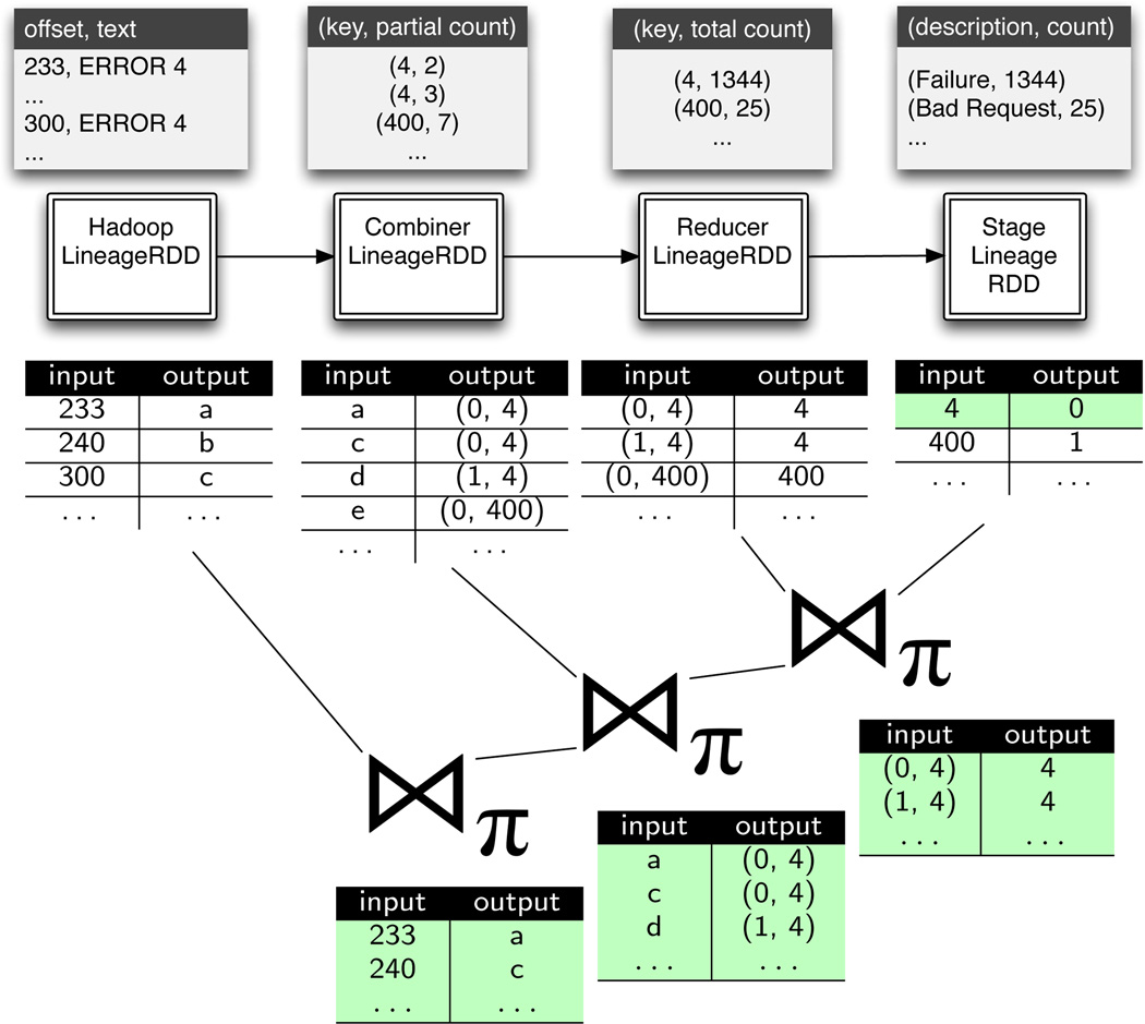
Figure 9 is a logical view of the data lineage that each agent captures in our running example from Figure 2. At the top of the figure, we show some example raw data corresponding to the HDFS input log, intermediate data, and final results. Recall, in the original running example, we were counting the number of occurrences for each error code. Here, we would like to trace back and see the actual log entries that correspond to a “Failure” (code =4), as shown in the Spark program of Figure 10.

Figure 9.

A logical trace plan that recursively joins data lineage tables, starting from the result with a “Failure” code, back to the input log records containing the error.

Figure 10.

Tracing backwards the “Failure” errors

The output is referenced by the reports RDD reference, which we use to select all “Failure” record outputs, and then trace back to the input HDFS log entries. Returning to Figure 9, the goBackAll transformation (Figure 10 line 2) is implemented by recursively joining the tables that associate the output record identifiers to input record identifiers, until we reach the data lineage at the HadoopLineageRDD agent. Notice that the inter-stage record identifiers (i.e., between CombinerLineageRDD and ReducerLineageRDD) include a partition identifier, which we use in Figure 11 to optimize the distributed join that occurs in the trace (described below). The example shows three joins—along with the intermediate join results—used to (recursively) trace back to the HDFS input.

Figure 11.

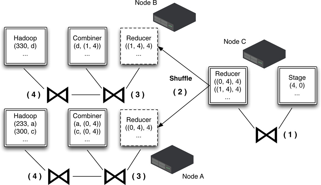
Distributed tracing plan that recursively joins data lineage tables distributed over three nodes. Each operation is labeled with a number. Operation (2) is an optimized shuffle that leverages the partition information in the record identifier to route trace record identifiers to the node containing the record in its output partition.

The logical plan generated by recursively joining lineage points is automatically parallelized by Titian. Figure 11 shows the distributed version of the previous example. Each agent data lineage is stored across three nodes. The trace begins at the Stage agent on node C, referencing result records with error code = 4. Tracing back to the stage input involves a local join (operation 1 in Figure 11). That join result will contain record identifiers that include a partition identifier e.g., identifier (0, 4) indicates that an error code = 4 occurs in partition 0, which we know to be on node A. We use this information to optimize the distributed join between the Combiner and Reducer agents. Specifically, the partition identifier routes (operation 2) the Reducer agent data lineage to the node that stores the given data partition e.g., partition 0 → A and partition 1 → B. The tracing proceeds on nodes A and B through two local joins (operations 3 and 4) that lead to the HDFS partition lines for error code = 4.

The optimized join described above required modifications to the Spark join implementation. Without this change, the Spark native join would shuffle both the Combiner and Reducer data lineage (in operation 2), since it has no knowledge of partitioning information. This would further impact the subsequent join with the Hadoop data lineage, which would also be shuffled. In Section 5, we show that our optimized join improves the tracing performance by an order of magnitude relative to a naïve join strategy.

4.6 Working with the Raw Data

LineageRDD references a subset of records produced by a native RDD transformation. When a native RDD transformation is called from a LineageRDD reference, Titian returns a native RDD that will apply the given transformation to the raw data referenced by the LineageRDD.

Figure 12 illustrates this feature by tracing back to log files that contain a “Failure”, and then selecting those that are specific to “Zookeeper” before printing.

Figure 12.

Native transformations on LineageRDD s

As before, we start the trace at reports and select the result containing the “Failure” error code. We then trace back to the HDFS log file input, which is referenced by the input LineageRDD. Calling filter on the input reference returns a native Spark FilterRDD that executes over the HDFS log file records that contain “Failure” codes⁴, and from that selects the ones containing “Zookeeper” failures. These are then collected at the driver by the collect action and printed.

The ability to move seamlessly between lineage data and raw data, in the same Spark session, enables a better interactive user experience. We envision this new Spark capability will open the door to some interesting use cases e.g., data cleaning and debugging program logic. It also provides elegant support for transformation replay from an intermediate starting point, on an alternative collection of records.

4.7 Discussion

Fault-tolerance

Our system is completely transparent to the Spark scheduler and in fact does not break the fault-tolerance model of Spark. During the capturing phase provenance data is materialized only when a task has completed its execution. In case of failure, no provenance is durably saved. During the tracing phase, LineageRDDs behave as a normal RDD and, as such, are resilient to failures.

Alternative Designs

Debugging systems such as IG [24] and Arthur [12] tag data records with a unique transformation id, and piggyback each tag downstream with its related record. This strategy can be easily implemented in Titian: each capturing agent generates the lineage data without storing it; lineage references are instead appended to a list and propagated downstream. The final stage capture point will then store the complete lineage data. In Section 5 we will compare this strategy (labeled as Titian-P, for Propagation) against the (distributed) Titian (Titian-D), and a naïve strategy that saves all the lineage into a unique centralized server (Titian-C). In Titian-C, agents write data lineage over an asynchronous channel to a centralized lineage master, which stores the data lineage in its local file system. The lineage master executes tracing queries, using a centralized version of LineageRDD, on the local data lineage files. Both Titian-C and Titian-P tradeoff space overheads, by aggregating lineage data into a more centralized storage, for a faster tracing time. An interesting area of future work would be an optimizer that is able to estimate the lineage size and select a version of Titian to use (centralized, decentralized, or propagated).

5. EXPERIMENTAL EVALUATION

Our experimental evaluation measures the added overhead in a Spark job caused by data lineage capture and the response time of a trace query. We compare Titian to Newt [21] and RAMP [18]. This required us to first integrate Newt with Spark. We also developed a version of RAMP in Spark using part of the Titian infrastructure. As in the original version, our version of RAMP writes all data lineage to HDFS, where it can be processed off-line. Moreover, in order to show the raw data in a trace, RAMP must also write intermediate data to HDFS. We report the overhead of RAMP when writing only the data lineage. Saving only the data lineage might be relevant when a user simply wants to trace back to the job input e.g., HDFS input.

5.1 General Settings

Datasets and Queries

We used a mixed set of workloads as suggested by the latest big data benchmarks [26]. All datasets used were generated to a specific target size. Following [18], we generated datasets of sizes ranging from 500MB to 500GB seeded by a vocabulary of 8000 terms that were selected from a Zipf distribution. We used these datasets to run two simple Spark jobs: grep for a given term and word count. We ported eight PigMix “latency queries” (labeled “L#”) to Spark for evaluating more complex jobs. These queries are categorized into three groups: aggregate queries (L1, L6, L11), join queries (L2, L3, L5), and nested plans queries (L4, L7). Due to space limitations, we report on a representative query from each class based on the worst-case performance. The input data for these queries was created by the PigMix generator, set to produce dataset sizes ranging from 1GB to 1TB.

Hardware and Software Configurations

The experiments were carried out on a cluster containing 16 i7 − 4770 machines, each running at 3.40GHz and equipped with 4 cores (2 hyper-threads per core), 32GB of RAM and 1TB of disk capacity. The operating system is a 64bit Ubuntu 12.04. The datasets were all stored in HDFS version 1.0.4 with a replication factor of 3. Titian is built on Spark version 1.2.1, which is the baseline version we used to compare against. Newt is configured to use MySQL version 5.5.41. Jobs were configured to run two tasks per core, for a potential total of 120 tasks running concurrently.

We report on experiments using three versions of Titian:

1. Titian-D stores data lineage distributed in the BlockManager local to the capture agent.

2. In Titian-P all agents, other than the last, propagate data lineage downstream. The final agent stores on the local Spark BlockManager the complete lineage of each individual data record as a nested list.

3. Titian-C agents write the lineage to a central server.

We expect Titian-P and -C to be less efficient than Titian-D during the capturing phase, but more effective in the tracing when the lineage data remains relatively small. Titian-P, in fact, propagate downstream the full lineage data of each individual record. This design is expensive when the size of the lineage is large. Conversely, executing a tracing query is as fast as recursively traversing a nested list. This operation can be faster than executing a (distributed) join while the size of the list remains reasonable. Concerning Titian-C, lineage data is uploaded to a centralized server, therefore we expect this version to have limited scalability.

As one might expect, Titian-D is the best strategy for big data lineage. It is also the plan strategy followed by Newt and RAMP. Therefore, in our evaluation, we compare Titian-D to Newt and RAMP, and separately compare Titian-D to Titian-P and Titian-C.

5.2 Data Lineage Capture Overheads

Our first set of experiments evaluate the overhead of capturing data lineage in a Spark program. We report the execution time of the different lineage capturing strategies in relation with the native Spark run time assumed as baseline. We executed each experiment ten times, and among the ten runs, we computed the trimmed mean by removing the top two and bottom two results and averaging the remaining six. In Titian(-D and -P) we store the data lineage using the Spark BlockManager with setting memory_and_disk, which spills the data lineage to disk when memory is full.

Grep and WordCount

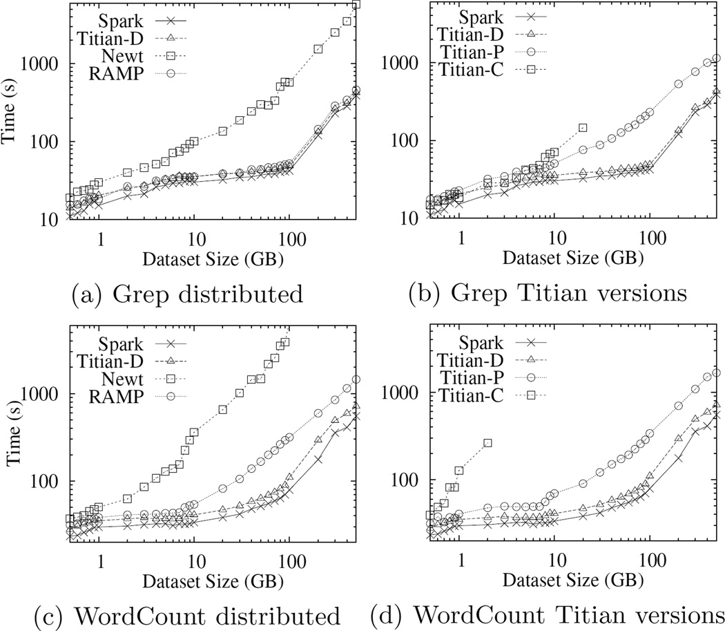
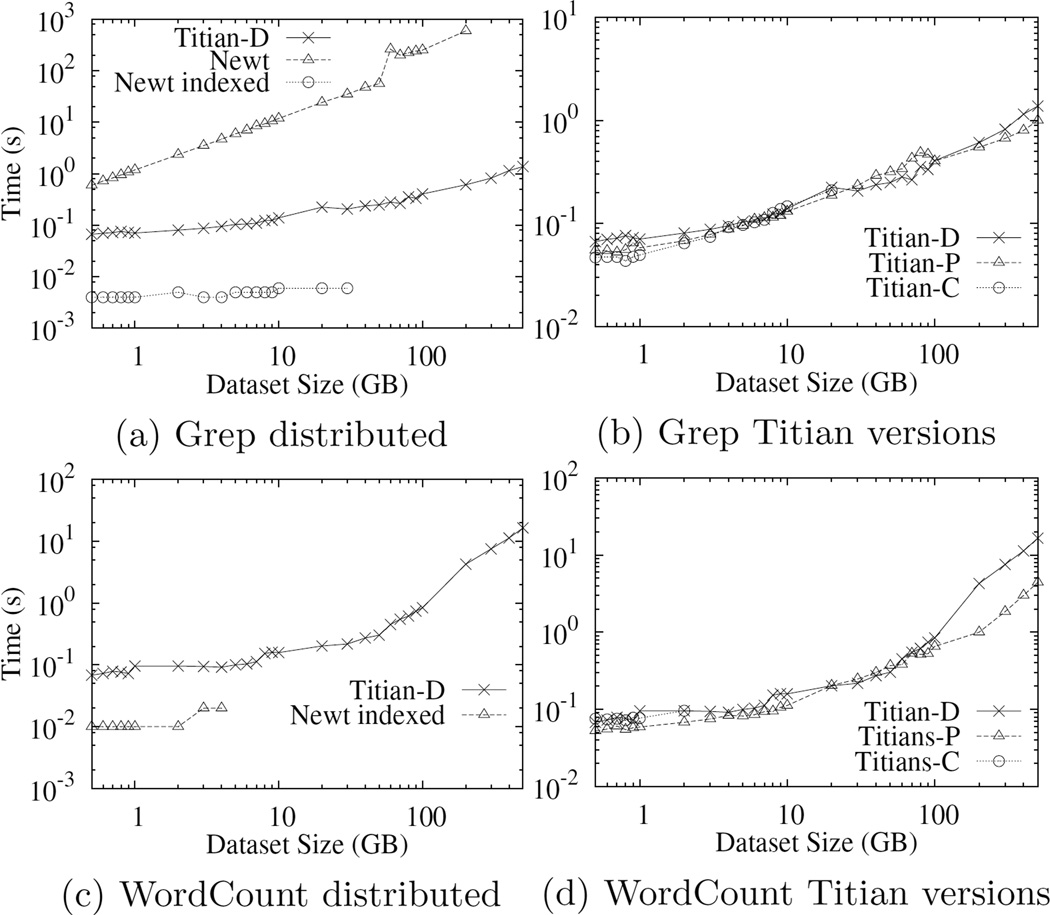
Figure 13(a) reports the time taken to run the grep job on varying dataset sizes. Both axes are in logarithmic scale. Under this workload Titian and RAMP incur similar overheads, exhibiting a run time of no more than a 1.35× the baseline Spark. However, Newt incurs a substantial overhead: up to 15× Spark. Further investigation led to the discovery of MySQL being a bottleneck when writing significant amounts of data lineage. Figure 13(b) compares the three versions of Titian executing the same job. On dataset sizes below 5GB, the three versions compare similarly. Beyond that, the numbers diverge considerably, with Titian-C not able to finish beyond 20GB.

Figure 13.

Lineage Capturing Performance for Grep and WordCount

Figure 13(c) reports the execution time for the word count job. For this workload, Titian-D offers the least amount of overhead w.r.t. normal Spark. More precisely, Titian-D is never more than 1.3× Spark for datasets smaller than 100GB, and never more than 1.67× at larger dataset sizes. The runtime of RAMP is consistently above 1.3× Spark execution time, and it is 2 − 4× slower than normal Spark for dataset sizes above 10GB. Newt is not able to complete the job above 80GB, and is considerably slower then the other systems. Moving to Figure 13(d), Titian-P performance is similar to RAMP, while Titian-C is not able to handle dataset sizes beyond 2GB.

Table 2 summarizes the time overheads in the grep and word count jobs for Titian-D, RAMP and Newt. Interestingly, for the WordCount workload, the run time of RAMP is 3.2× Spark at 50GB and decreases to 2.6× at 500GB. From Figure 13(c) we can see that is because Spark performance decreases. After an in depth analysis, we found that scheduler-time increases considerably for dataset greater than 100GB. Conversely, in RAMP the computation is bounded by the offload of the lineage data to HDFS.

Table 2.

Runtime of Titian-D, RAMP and Newt for grep and word count jobs as a multiplier of Spark execution time.

	Titian − D		RAMP		Newt
dataset	grep	wc	grep	wc	grep	wc
500MB	1.27×	1.18×	1.40×	1.34×	1.58×	1.72×
5GB	1.18×	1.14×	1.18×	1.32×	1.99×	4×
50GB	1.14×	1.22×	1.18×	3.2×	8×	29×
500GB	1.1×	1.29×	1.18×	2.6×	15×	inf

Space Overhead

In general, the size of the lineage increases proportionally with the size of the dataset. More specifically, we found that the lineage size is usually within 30% of the size of the input dataset, with the exception of word count on datasets bigger than 90GB, where the lineage size is on average 50% of the size of the initial dataset. In computing the space overhead, we took into account both the size of the actual lineage, and the overhead introduced by the provenance data into the shuffle. For big datasets, in some uses case (e.g., word count) lineage data does not completely fit into memory, and therefore a part of it is spilled to disk. Note that lineage data going to disk does not introduce slowdown during lineage capturing because lineage is materialized asynchronously.

PigMix Queries

The results for Titian-D on the three Pig- Mix queries are constantly below 1.26× the baseline Spark job. Figures 14(a), (b) and (c) show the running times for queries L2, L6, and L7. We summarize the results for each query below.

Figure 14.

Lineage Capturing Performance for Pigmix queries

L2

We observe that Titian-D exhibits the least amount of overhead for all dataset sizes, with Titian-P adding slightly more (up to 40%) overhead. Titian-C is only able to execute dataset size 1GB at around 2.5× Spark execution time. RAMP is on par with Titian-P for 1GB and 10GB datasets. Its running time degrades at 100GB (around 2.4× the Spark runtime) and it is not able to complete on the 1TB dataset. Newt incurs significant overhead throughout, and is not able to complete on the 100GB and 1TB datasets.

L6

Titian-D-P are able to complete this query for all dataset sizes. Titian-D is constantly less that 1.2× Spark execution time, while the execution time for Titian-P goes up to 2× in the 1TB case. Titian-C is able to complete up to the 100GB dataset with a run time ranging from 1.1× (at 1GB) to 1.95× (at 100GB). RAMP and Newt are able to complete up to the 100GB case, with an average running time of 1.16× Spark in RAMP, and in Newt we see a 7× slowdown w.r.t. Spark.

L7

The general trend for this query is similar to L2: Titian-D-P and RAMP have similar performance on the 1GB and 10GB datasets. For the 100GB dataset, RAMP execution time is 2.1× the baseline Spark. Titian-C can only execute the 1GB dataset with an execution of 2.6× Spark. Newt can only handle the 1GB and 10GB datasets at an average time of 3.6× over baseline Spark.

5.3 Tracing

We now turn to the performance of tracing data lineage, starting from a subset of the job result back to the input records. We compare against two configurations in Newt: (1) that indexes the data lineage for optimizing the trace, and (2) no indexes are used. The later configuration is relevant since indexing the data lineage can take a considerable amount of time e.g., upwards of 10 minutes to one hour, depending on the data lineage size.

The experiments described next were conducted as follows. First, we run the capturing job to completion. For Newt, the first step also includes building the index (when applicable). We do not report these times in our plots. Next, we randomly select a subset of result records, and from there trace back to the job input. The trace from result to input is repeated 10 times, on the same selected result, and we report the trimmed mean. We only report on backward traces since the forward direction, from input to output, exhibits similar results. We do not report the results for tracing queries taking more that 10 minutes. Also, for the Newt case with indexes, we do not report results when the index building time exceeds 1 hour.

Optimizing Spark Join for Tracing

In Section 4.5 we have described our modification to the Spark join operator to leverage the partition identifier information embedded in the record identifier.

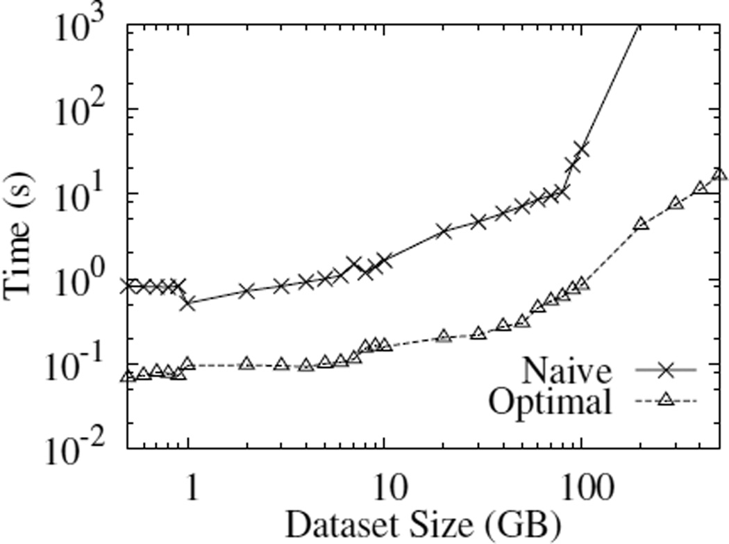
This optimization avoided the naïve join strategy, in which the data lineage, stored in the BlockManager, would be fully shuffled in every join. Figure 15 shows the benefits of this optimization when tracing the data lineage from the word count job. The naïve join is around one order of magnitude slower than the optimal plan up to 80GB. Beyond that, the naïve performance degrades considerably, with the trace at 200GB taking approximately 15 minutes, compared to the optimal 5 seconds. The naïve join strategy is not able to complete traces above 200GB.

Figure 15.

naïve vs optimal plan

Trace Grep and WordCount

The time to trace backward one record for grep is depicted in Figure 16(a). In the Newt case, the query to compute the trace backward is composed of a simple join. Not surprisingly, when relations are indexed the time to compute a full trace is small. When the relations are not indexed, the time to execute the query increases to 10 minutes. Tracing queries over Titian-D scale linearly from 0.07 seconds (at 500MB) to 1.5 seconds (at 500GB). Figure 16(b) compares the three versions of Titian. As expected, Titian-P and -C are slightly faster than Titian-D since the data lineage is more localized and not large.

Figure 16.

Tracing time for grep and word count

Figure 16(c) shows the execution time for retrieving the full lineage of a single record for word count. Newt without indexes is not able to complete any trace in less than 10 minutes. When the data lineage is indexed, Newt is able to trace up to the 5GB dataset, after which the index build time reached one hour. Titian-D executed the 1GB dataset trace in 0.08 seconds, and it took no more than 18 seconds for larger datasets. In Figure 16(d) Titian-D-P-C have similar performances for small dataset sizes, while Titian-P outperform Titian-D by a factor of 4 for bigger sizes.

PigMix Queries

Figures 14(a), (d) and (e) show the tracing time for PigMix queries L2, L6 and L7 respectively.

L2

We were able to execute the non-indexed Newt trace only for the 1GB (13 seconds) and 10GB datasets (more than 200 seconds). The indexed version maintains constant performance (5 milliseconds) up to 100GB, but failed to build the index in less than one hour for 1TB dataset. All the Titian versions exhibit similar performance, executing the trace in a few hundreds of milliseconds for smaller datasets (Titian-P has the best result with 0.1 seconds for the 1GB dataset), and few seconds for the bigger one (Titian-P has again the best result with 2.1 seconds for the 1TB dataset).

L6

For this aggregate query, Newt is not able to complete any tracing query under the threshold of 600 seconds. The indexed version still maintains constant performance and up to 100GB. Titian-C is able to complete both the 1GB and 10GB workloads with a tracing time respectively of 0.25 and 0.57 seconds. Titian-D and -P have comparable performance up to 10GB. For 100GB Titian-P performs relatively better than Titian-D (0.6 seconds versus 0.8), while for the 1TB Titian-D is 6 times faster (55 against 337 seconds).

L7

The trend for this query follows the one of query L6, although the tracing time is in general two time faster. For instance, Titian-D takes 25 seconds for tracing one record over the 1TB dataset, while Titian-P takes 150 seconds.

Discussion

Compared to query L2, tracing one record for the 1TB dataset in L6 and L7 is more than an order of magnitude slower since these are aggregate queries. Recall, to minimize the the memory footprint, Titian-D and -P save lineage in nested format i.e., a single top-level identifier is used to reference the set of identifier corresponding to the record group. The un-nesting (dereferencing) of the data lineage is an expensive operation for tracing through aggregate operators, especially in the Titian-P case.

5.4 Show me the Data

Measuring the efficiency of replay includes the performance of tracing, retrieving the data records referenced by the lineage, and the cost of re-computation. In this section, we focus on the performance of the second step i.e., raw data retrieval.

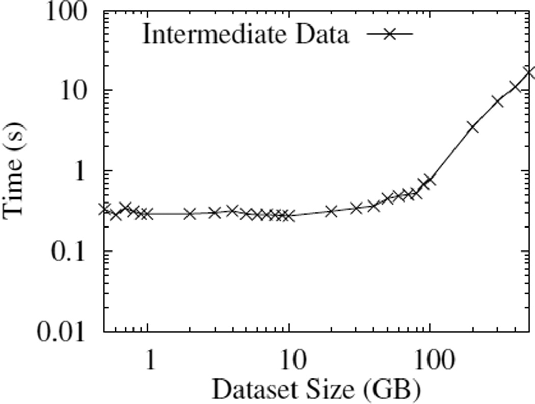
Figure 18 depicts the time of retrieving an intermediate data record from its lineage identifier. This operation involves reading the intermediate data partition, then scanning to the data record location. As the figure shows, for datasets less than 70GB, this operation takes less than one second. Beyond 70GB, the time increases up to 27 seconds for the 500GB case. This increase in access time is due to the increased size of the intermediate data partitions as we scale up the experiment. As future work, we plan to mitigate this effect by subdividing intermediate data partitions and embedding a reference pointer in the lineage identifier.

Figure 18.

Data retrieval performance

6. RELATED WORK

There is a large body of work that studies techniques for capturing and querying data lineage in data-oriented workflows [5, 6, 8, 11, 17, 22]. Data provenance techniques have also been applied in other fields such as fault injection [4], network forensics [28], and distributed network systems analysis [29]. In this paper we have compared Titian against the approaches relevant to DISC workflows [18, 21].

Inspector Gadget (IG) [23] defines a general framework for monitoring and debugging Apache Pig programs [24]. IG introspects the Pig workflow with monitoring agents. It does not come with full data lineage support, but rather it provides a framework for tagging records of interest as they are passed through the workflow. In this setting, programmers embed code in the monitoring agents that tag records of interest, while IG is responsible for passing those tags through to the final output.

Arthur [12] is a Spark library that can re-execute (part of) the computation to produce the lineage information on demand. Although such an approach introduces zero overhead on the target dataflow, it sacrifices the ability to provide interactive analysis capabilities of tracing queries, as all queries are done in post-mortem sessions. Similarly to IG (and to Titian-P) Arthur uses tagging techniques to generate and propagate lineage data, but it requires re-running queries after instrumentation.

A common pattern for provenance systems is to use different languages for querying the data and querying the lineage [20, 6]. In our system instead we provide a lightweight extension of the transformations already provided by Spark. In this way we are able to provide users with a uniform language for data and lineage analysis. To our knowledge only [14] provides a similar feature, in the context of relational database systems.

7. CONCLUSION AND FUTURE WORK

We began this work by leveraging Newt for data provenance support in Apache Spark. During this exercise, we ran into some usability and scalability issues, mainly due to Newt operating separately from the Spark runtime. This motivated us to build Titian, a data provenance library that integrates directly with the Spark runtime and programming interface. Titian provides Spark programmers with the ability to trace through the intermediate data of a program execution, at interactive speeds. Titian’s programming interface extends the Spark RDD abstraction, making it familiar to Spark programmers and allowing it to operate seamlessly through the Spark interactive terminal. We believe the Titian Spark extension will open the door to a number of interesting use cases, including program debugging [16], data cleaning [19], and exploratory data analysis.

In the future, we plan to further integrate Titian with the many Spark high-level libraries, such as GraphX (graph processing) [15], MLlib (machine learning) [2], and Spark SQL (database-style query processing) [7]. We envision each high-level library will motivate certain optimization strategies and data lineage record requirements e.g., how machine learning features and models associate with one another.

Figure 17.

Lineage Tracing Performance for PigMix Queries