Calibration and Evaluation of Ultrasound Thermography using Infrared Imaging

Abstract

Real-time monitoring of the spatiotemporal evolution of tissue temperature is important to ensure safe and effective treatment in thermal therapies including hyperthermia and thermal ablation. Ultrasound thermography has been proposed as a non-invasive technique for temperature measurement, and accurate calibration of the temperature-dependent ultrasound signal changes against temperature is required. Here we report a method that uses infrared (IR) thermography for calibration and validation of ultrasound thermography. Using phantoms and cardiac tissue specimens subjected to high-intensity focused ultrasound (HIFU) heating, we simultaneously acquired ultrasound and IR imaging data from the same surface plane of a sample. The commonly used echo time shift-based method was chosen to compute ultrasound thermometry. We first correlated the ultrasound echo time shifts with IR-measured temperatures for material-dependent calibration and found that the calibration coefficient was positive for fat-mimicking phantom (1.49 ± 0.27) but negative for tissue-mimicking phantom (− 0.59 ± 0.08) and cardiac tissue (− 0.69 ± 0.18 °C-mm/ns). We then obtained the estimation error of the ultrasound thermometry by comparing against the IR measured temperature and revealed that the error increased with decreased size of the heated region. Consistent with previous findings, the echo time shifts were no longer linearly dependent on temperature beyond 45 – 50 °C in cardiac tissues. Unlike previous studies where thermocouples or water-bath techniques were used to evaluate the performance of ultrasound thermography, our results show that high resolution IR thermography provides a useful tool that can be applied to evaluate and understand the limitations of ultrasound thermography methods.

INTRODUCTION

Thermal therapies have been used in treating benign and malignant diseases. For example, hyperthermia, in which tissue temperature is elevated to 41 – 45 °C, has been used for cancer treatment in conjunction with radiation therapy and chemotherapy (Dewhirst et al. 1997; Franckena et al. 2009; Ryu et al. 2004; Zagar et al. 2010). Elevated temperatures are also exploited for controlled drug release (Staruch et al. 2011). High temperature thermal ablations are employed to destruct diseased tissue through induction of coagulative necrosis (Goldberg et al. 2000). Among the common heat sources for thermal therapies including high-intensity focused ultrasound (HIFU), radiofrequency (RF) wave, microwave, and laser, HIFU uses ultrasound energy and provides a noninvasive modality capable of inducing localized heating in deep tissue regions without affecting intervening tissue (Crouzet et al. 2010; Kennedy 2005).

Real-time temperature information in tissue is important for guiding thermal therapies. Traditional temperature measurements using thermocouples placed at discrete locations may not be feasible for clinical implementation due to the requirement of thermocouple insertion. The most promising noninvasive techniques for in vivo temperature measurement are magnetic resonance imaging (MRI) and ultrasound imaging. MR thermometry is based on temperature-sensitive MR parameters such as T₁ and T₂ relaxation time, proton resonance frequency, and proton diffusion coefficient (Rieke and Butts Pauly 2008; Rivens et al. 2007). Although capable of millimeter spatial resolution and temperature sensitivity of a few degrees (Jolesz 2009; Rivens et al. 2007), the acquisition duration of MRI (few seconds/frame) (Kopelman et al. 2006) may limit its use in treatments involving rapid tissue heating (Rivens et al. 2007) or result in extended treatment time (Wu 2006). In addition, MR-compatible treatment devices are also required. High cost of MRI scanners, claustrophobia and discomfort experienced by some patients in closed-bore systems, and the lack of portability of MRI systems are additional disadvantages that could restrict the widespread use of the technology for thermal therapies (Kennedy 2005).

In contrast, ultrasound imaging is non-ionizing, highly portable, and at a lower cost. Ultrasound imaging systems are also readily compatible to various types of thermal treatment devices, especially for HIFU procedures, for which dual-mode ultrasound transducers may be conveniently used for both imaging and thermal therapy (Owen et al. 2010). Ultrasound thermography measures tissue temperature by detecting temperature-dependent changes in ultrasound backscattered signals. A variety of signal processing techniques have been explored, including methods based on ultrasound echo time shifts (Anand et al. 2007; Liu and Ebbini 2010; Maass-Moreno and Damianou 1996; Maass-Moreno et al. 1996; Seip et al. 1996; Simon et al. 1998; Varghese et al. 2002), changes in backscattered energy (Arthur et al. 2010; Straube and Arthur 1994; Tsui et al. 2012a), and spectral parameters (Amini et al. 2005). There are several challenges in applying ultrasound thermometry. In order to estimate temperature accurately, sufficient signal-to-noise (SNR) level is required to detect small changes in ultrasound backscattered signals, particularly in tissues with low fat content (Miller et al. 2002). Also, the relation between temperature and changes in ultrasound backscattered signals can vary in different ranges of temperatures. As most methods depend on a linear relation which is valid up to approximately 50 °C, most studies were investigated in the hyperthermia range.

More importantly, ultrasound thermography requires calibration to determine quantitatively the relationship of ultrasound signals with temperature in the specific tissue type of interest. Such calibrations may be performed with global or uniform heating of specimens submerged in water-bath with controlled temperatures (Arthur et al. 2010; Liu et al. 2009; Simon et al. 1998; Tsui et al. 2012b). However, water-bath heating requires prolonged time to allow specimens to reach a uniform temperature. For example, for a 20 °C temperature range, measurements can take several hours (Simon et al. 1998). To obtain independent temperature measurement, thermocouples are often used and they need to be inserted into the specimen at locations in the field of view of ultrasound imaging (Maass-Moreno et al. 1996). Yet thermocouples are invasive and can be disruptive to the HIFU field, and may introduce error in measurements due to viscous heating and thermal conduction by thermocouples themselves (Clarke and ter Haar 1997; Fry and Fry 1954; Morris et al. 2008; Rivens et al. 2007). In addition, measurements at discrete and sparse locations (Liu et al. 2009; Simon et al. 1998) provide limited spatial resolution often insufficient for performance evaluation of ultrasound thermometry, particularly in HIFU thermal ablations where temperature gradient is relatively large.

In this study, we demonstrate the use of infrared (IR) thermography for calibrating and evaluating ultrasound thermography with spatiotemporal temperature information unavailable using thermocouples. IR thermography typically uses mid-IR (3 – 5 μm) and long-IR (8 – 12 μm) spectrum for thermal imaging (Diakides et al. 2008). Although limited to surface measurements, IR thermography is easy to implement, and can readily measure temperature with high spatial and temporal resolution (< 100 μm and > 100 Hz) without contact.

These advantages motivated the use of IR thermography for diagnosis and treatment monitoring, as demonstrated by applications in oncology (breast cancer, skin diseases), skin burns, vascular disorders, surgery, tissue viability, and mass screening (Diakides et al. 2008; Ogan et al. 2003; Song et al. 2009). IR imaging has been exploited to visualize the heat deposition from HIFU transducers (Bobkova et al. 2010; Hand et al. 2009; Patel et al. 2008) and to record temperature profiles during HIFU exposures to optimize ultrasound parameters (Qiu et al. 2009; Song et al. 2005). IR thermography has also been proposed as an alternative way to calibrate transducers by converting the spatiotemporal IR temperature measurement to spatial ultrasound beam intensities through mathematical derivations (Giridhar et al. 2012; Myers and Giridhar 2011). We have also demonstrated its use for identifying the temperature characteristics indicative of tissue coagulation and cavity formation in HIFU application (Hsiao et al. 2013).

The goal of this study is to develop a method and an experimental platform using IR to aid the development of ultrasound thermometry. We implemented simultaneous and correlated IR thermography and ultrasound imaging, and measured the spatiotemporal temperature changes and ultrasound backscattered signals in the same surface plane of the phantoms or tissue specimens subjected to HIFU heating. We employed an echo time shifts method using cross-correlation speckle tracking for ultrasound thermography (Pernot et al. 2004; Seip et al. 1996; Simon et al. 1998; Varghese et al. 2012). We first used the echo time shifts and IR measured temperature for material-dependent calibration, and then applied the calibration coefficients to the ultrasound speckle tracking method to estimate temperature. Finally, by comparing the estimated temperature with the IR-measurement, we determined the spatiotemporal evolution of error in ultrasound thermography.

MATERIALS AND METHODS

Ultrasound echo time shift due to heating

For pulse-echo operation, the time of arrival, τ, of the ultrasound signal from a location at axial depth y, without the effects of thermal expansion, can be calculated from $\tau \left(y\right)=2{\displaystyle {\int }_0^y\frac{1}{c\left(\theta \left(\xi \right)\right)}}d\xi$, where c(θ(ξ)) is the speed of sound as a function of the local temperature θ(ξ) at depth ξ (Simon et al. 1998). With isotropic free thermal expansion under temperature changes, a local element volume within a specimen will expand in all directions outward from the center of the heating zone. Assume the expansion is interrogated by pulse-echo ultrasound along an A-line intersecting the center of heating zone, the anterior portion of the local volume will move toward the detecting ultrasound transducer while the posterior portion of the local volume will move away from the detecting transducer, as shown in Fig. 1.

Figure 1.

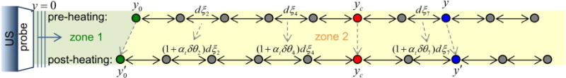
Diagram of ultrasound echo time shifts after HIFU heating. zone 1 is the temperature constant zone from the transducer surface (y = 0) to y₀; zone 2 is the heating zone. dξ denotes the distance between two scatters, α_t the linear coefficient of thermal expansion, δθ the temperature changes, and y_c the location of the spatial peak temperature rise.

Assuming the effect of transducer self-heating is negligible, we calculate τ from an ultrasound scatterer at location y by dividing the ultrasound beam path into two segments (Fig. 1). The first segment, the zone without temperature change, includes the region from the transducer surface (y = 0) up to y₀ where no temperature changes occur, and the second segment is the heating zone which includes locations from y ≥ y₀ with temperature changes δθ(ξ) at each depth ξ. Thus the baseline time of arrival τ₀(y) from a scatter located at y before heating is

$${\tau }_0\left(y\right)=2{\displaystyle {\int }_0^y\frac{1}{c_0}d\xi =\frac{2y_0}{c_0}}+2{\displaystyle {\int }_{y_0}^y\frac{1}{c_0}}d\xi ,$$ (1)

where c₀ is the speed of sound at baseline temperature θ₀. For HIFU heating, we can express y₀ using the HIFU focus or the center of the focal zone y_c as $y_0=y_c-{\displaystyle {\int }_{y_0}^{y_c}d\xi }$. Therefore with temperature changes, the scatterer at y shifts in location to y′ with a time of arrival

$$\tau \left(y\prime \right)=\frac{2{y\prime }_0}{c_0}+2{\displaystyle {\int }_{y_0}^y\frac{1+{\alpha }_t\left(\theta \left(\xi \right)\right)\cdot \delta \theta \left(\xi \right)}{c\left(\theta \left(\xi \right)\right)}}d\xi ,$$ (2)

where y₀′ is the new location for y₀ after heating and ${y\prime }_0=y_c-{\displaystyle {\int }_{y_0}^{y_c}\left(1+{\alpha }_t\left(\theta \left(\xi \right)\right)\cdot \delta \theta \left(\xi \right)\right)}\cdot d\xi \cdot {\alpha }_t\left(\theta \left(\xi \right)\right)$ is the linear coefficient of thermal expansion at depth ξ with temperature θ(ξ). The echo time shift δτ(y) due to heating can then be computed by subtracting Eq. 2 from Eq. 1:

$$\delta \tau \left(y\right)\tau \left(y\prime \right)-{\tau }_0\left(y\right)=-\frac{2}{c_0}{\displaystyle {\int }_{y_0}^{y_c}\left[{\alpha }_t\left(\theta \left(\xi \right)\right)\cdot \delta \theta \left(\xi \right)\right]}d\xi +2{\displaystyle {\int }_{y_0}^y\left[\frac{1+{\alpha }_t\left(\theta \left(\xi \right)\right)\cdot \delta \theta \left(\xi \right)}{c\left(\theta \left(\xi \right)\right)}-\frac{1}{c_0}\right]}d\xi ,$$ (3)

which accounts for the effects of heating-induced changes of the speed of sound and thermal expansion. Our derived expression for the echo time shift due to temperature changes differs from Simon et al.’s paper (1998), in which they derived $\delta \tau \left(y\right)=2{\displaystyle {\int }_0^y\left[\frac{1+{\alpha }_t\left(\theta \left(\xi \right)\right)\cdot \delta \theta \left(\xi \right)}{c\left(\theta \left(\xi \right)\right)}-\frac{1}{c_0}\right]}d\xi$. This is because we assume isotropic free expansion which accounts for thermal expansion towards the transducer.

Ultrasound thermometry

We describe here the process of estimating temperature from the gradient of the echo time shift. By differentiating Eq. 3 with regard to depth, we obtain the gradient of the echo time shift

$$\frac{\partial \left(\delta \tau \left(y\right)\right)}{{\partial }_y}=2\left[\frac{1+{\alpha }_t\left(\theta \left(y\right)\right)\cdot \delta \theta \left(y\right)}{c\left(\theta \left(y\right)\right)}-\frac{1}{c_0}\right].$$ (4)

Eq. 4 is identical with Simon et al.’s (1998) derivation because the first term in the right-hand side of Eq. 3 does not depend on depth variable y. For most biological materials with temperature 20 – 40 °C, a linear relationship can usually be assumed (Bamber 2004; Duck 1990) for the speed of sound and temperature:

$$c\left(\theta \left(y\right)\right)=c_0\cdot \left(1+\beta \cdot \delta \theta \left(y\right)\right),$$ (5)

where ${\beta =\frac{1}{c_0}\frac{\partial c(y,\theta )}{\partial \theta }|}_{\theta ={\theta }_0}$. Although α_t can be a function of temperature (Duck 1990), for simplicity we assume that it is constant over the temperature range under investigation. Thus for small thermal expansion, |β·δθ|≪1, Eq. 4 can be rewritten as

$$\frac{\partial \left(\delta \tau \left(y\right)\right)}{\partial y}\approx \frac{2}{c_0}\cdot \left({\alpha }_t-\beta \right)\cdot \delta \theta \left(y\right),$$ (6)

allowing estimation of temperature change from the gradient of temperature change and a material dependent coefficient (Pernot et al. 2004; Seip et al. 1996; Simon et al. 1998; Varghese et al. 2012):

$$\delta \theta \left(y\right)=\frac{c_0}{2}\cdot k\cdot \frac{\partial \left(\delta \tau \left(y\right)\right)}{\partial y},$$ (7)

where k = 1/(α_t − β) is material dependent and needs to be determined via calibration.

Calibration of ultrasound thermometry

In order to determine the calibration coefficient k, we integrate the temperature changes (Eq. 7) from y₀ to y along the A-line to obtain the spatial cumulative temperature-rise, cum[ΔT_IR(y)] (°C-mm), as a linear function of echo time shift

$$\mathit{cum}\left[\mathrm{\Delta }{T}_{IR}\left(y\right)\right]={\displaystyle {\int }_{y_0}^y\delta \theta \left(\xi \right)}\cdot d\xi =\frac{c_0}{2}\cdot k\cdot {\displaystyle {\int }_{y_0}^y\frac{\partial \left(\delta \tau \left(\xi \right)\right)}{\partial \xi }}\cdot d\xi =\frac{c_0}{2}\cdot k\cdot \left[\delta \tau \left(y\right)-\delta \tau \left(y_0\right)\right]=a\cdot \delta \tau \left(y\right)+b,$$ (8)

where a = c₀·k/2 and b = − δτ(y₀)·c₀·k/2. These parameters, thus the calibration coefficient k, will be determined from experimentally measured echo time shifts and spatial distribution of temperature.

Experimental sample preparation

Ex vivo porcine cardiac tissue specimens were obtained from a local abattoir and cut into square-shaped samples with a thickness of 15–17 mm. Two different types of phantoms were fabricated in this study. The first one was a water-based graphite-in-gelatin phantom to mimic typical biological tissue, and the other was an oil-based fat-mimicking phantom. These phantoms were chosen due to their differences in how temperature affects the sound speed and thermal expansion.

Tissue-mimicking phantom

Graphite-in-gelatin phantom (Madsen et al. 1978) was constructed as tissue mimicking phantom using 0.1 g/ml gelatin powder, 0.07 g/ml graphite powder, 0.0024 g/ml p-toluic acid, and 7% 2-propanol mixed in deionized water. The mixture was heated slowly on a hot plate with magnetic stirrer until the powder was fully dissolved. The solution was placed in a vacuum chamber for several minutes to remove gas bodies before it was poured into an agar mold.

Fat-mimicking phantom

Fat-mimicking phantom (Madsen et al. 1982) was fabricated using a gelatin solution and an oil solution which were heated separately before mixing them together. The gelatin solution consisted 0.1 g/ml gelatin powder and 1.67% 2-propanol in deionized water, and the oil solution consisted 25% olive oil and 16.67% castor oil (all concentrations were calculated based on the final mixture volume). After the gelatin solution became clear, the oil solution was slowly mixed into the gelatin solution, during which 1.67% detergent was added. The mixture was stirred thoroughly and was placed in the vacuum chamber for several minutes to remove gas bodies before it was poured into an agar mold.

To house the experimental samples, we fabricated agar-based molds for simultaneous and correlated ultrasound imaging and IR thermography of the sample subjected to HIFU heating. The agar-based molds were made with 1% mg/ml agar powder and deionized water. After the molds completely solidified, a sample (phantom or tissue specimen) was placed inside the molds and fixed in position with additional agar solution.

Experimental setup and design

Our experimental setup (Fig. 2A) includes an IR camera (Silver 5600, FLIR Systems, Boston, MA, USA), an ultrasound imaging system (Vevo 770; Visualsonics, Toronto, ON, Canada), and a HIFU system. The IR camera, sensitive to the mid-IR wavelength (3 – 5 μm), has a temperature measurement accuracy of ± 1 °C and a resolution of 0.01 °C (given a perfect blackbody). Conversion from IR radiance to temperature was performed using the manufacturer’s calibration and non-uniformity corrections. Ultrasound imaging used a high-frequency scanhead (RMV 707B) with a 30 MHz center frequency, 12.7 mm focal distance, 2.2 mm 6 dB depth of focus, 55 μm axial resolution, and a 115 μm lateral resolution. The raw radiofrequency (RF) backscattered signals from the Vevo system were acquired using a digitizing oscilloscope (54830B, Agilent, Santa Clara, CA) at 500 Msample/s. The HIFU system consisted of a HIFU transducer, a function generator (33220A, Agilent, CA), and a power amplifier (75A250, Amplifier Research, Souderton, PA). Two different HIFU transducers were used in the phantom experiments (3.98 MHz center frequency, F = 1, Blatek, Inc., State College, PA) and the tissue experiments (2 MHz center frequency, F = 0.98, Sonic Concepts, Inc., Bothell, WA), respectively. The HIFU transducers, calibrated using a hydrophone (HNR-0500, Onda, Sunnyvale, CA) have a −6 dB focal dimension of (width × length) 0.7 mm × 5 mm and 0.8 mm × 7 mm, respectively. The spatial peak temporal average intensity (I_spta) was also measured for both transducers with input powers used in this study.

Figure 2.

(A) Schematic illustration of experimental setup. (B) Photo of the ultrasound (US) probe and fat-mimicking phantom embedded in an agar mold. The region of interest is indicated by the red box. (C) and (D) show the corresponding ultrasound gray scale (GS) image and IR-measured temperature T_IR. The alignment reference pin (L-shaped wire) can be seen on both images at around 6.3 mm depth.

Emissivity measurement for IR thermography

Emissivity determines the efficiency of a body to radiate and absorb energy, and is defined as the ratio of the radiation emitted by the object to the radiation emitted by a blackbody at the same temperature (Incropera et al. 2007). A dimensionless parameter, it has a value between 0 and 1 with 1 representing perfect blackbody. For accurate conversion from IR radiance to temperature, knowledge of the emissivity of the imaged object is required. We measured the emissivity of all samples using the black tape method (Madding 2003) with the IR camera perpendicularly facing the sample surface. The Scotch Super 33+ Vinyl Electrical Tape (3M Company, St. Paul, MN) with a known emissivity of 0.95 was used.

Simultaneous and synchronized IR and ultrasound imaging of HIFU heating

As shown in Fig. 2A, the HIFU transducer was submerged in water facing up towards the specimen in the agar-mold placed above. The focus of the HIFU transducer was placed near the top surface of the specimen by employing a pulse-echo method to locate the specimen-air interface. The surface of the specimen was above the water level to allow measurement of HIFU induced temperature increase using the IR camera positioned above and facing downward. Orthogonal with the IR imaging, the ultrasound imaging probe was placed horizontally at a vertical location close to the specimen surface (Fig. 2B) to enable imaging of the same surface plane as the IR measurement. Spatial alignment of the IR and ultrasound imaging was achieved by using an L-shaped thin metal wire with one leg inserted into the specimen and the other placed on the specimen surface, allowing the wire target to be visible under both imaging modalities. Temporal synchronization was achieved using the “line trigger” and “frame trigger” output signal from the Vevo system to trigger the oscilloscope, HIFU system, and IR camera through a delay-pulse generator (Model 565, Berkeley Nucleonics Corp., San Rafael, CA).

RF data corresponding to B-mode ultrasound images consisted of 32 A-lines with a separation of 27.5 μm between adjacent A-lines were acquired at a frame rate of 34.4 Hz. HIFU exposures (34.4 Hz pulse repetition frequency, 51.7 % duty cycle, 0.84 s total duration, free field I_spta 180 – 700 W/cm²) were initiated 12 ms after the B-mode “frame trigger” to interleave with the imaging pulses to avoid interference. B-mode images were acquired for 6 frames before, 30 frames during, and 27 frames after HIFU exposures. IR images of the specimen surface were acquired continuously at 50 Hz frame rate. Four sets of experiments were performed using the tissue-mimicking phantom, five the fat-mimicking phantom, and fifteen sets using cardiac tissue specimens (n = 3 samples). All experiments were conducted at room temperature (20 °C). Maximum temperature rise was around 10 and 15 °C in tissue-mimicking and fat-mimicking phantoms, and about 75 °C in cardiac tissues, respectively.

Image and data analysis

All image analysis and computations were performed using MATLAB (R2012b, Mathworks, Natick, MA) offline. For both IR and ultrasound images, t = 0 was set to the start of HIFU application. Orientation of the x- and y-axis are shown in Fig. 2B, with x = 0 corresponding to the center A-line of a B-mode image and y = 0 corresponding to the specimen-agar mold interface closer to the ultrasound transducer. The 1D model presented in the previous section was applied to the RF data of each A-line in a B-mode image, thus notation of lateral location ‘x’ is only needed when 2D spatial interpolation or filtering is involved.

Cumulative temperature-rise and center of heating

The temperature-rise, ΔT_IR, at location (x, y) and time t is calculated from the temperature (T_IR) measured using IR thermography

$$\mathrm{\Delta }{T}_{\mathrm{IR}}\left(x,y,t\right)=T_{\mathrm{IR}}\left(x,y,t\right)-T_0\left(x,y,t\le 0\right),$$ (9)

where baseline temperature T₀(x, y, t ≤ 0) is the average of the temperatures from – 0.62 to 0 sec before HIFU application. The spatial “cumulative temperature-rise” from y₀ to y, cum[ΔT_IR(y)], as described in Eq. 8, can be estimated using the following equation

$$\mathit{cum}\left[\mathrm{\Delta }{T}_{IR}\left(y\right)\right]={\displaystyle {\int }_{y_0}^y\delta \theta \left(\xi \right)}d\xi \approx {\displaystyle \sum _{y_0}^y\mathrm{\Delta }{T}_{IR}}\left(y\right)\cdot \mathrm{\Delta }{y}_{IR},$$ (10)

where Δy_IR may be chosen as the pixel size of the IR images, and y₀ is the depth when ΔT_IR(y ≤ y₀) = 0 which can be determined from the IR images.

Both ΔT_IR(x, y) and cum[ΔT_IR(x, y)] at each t were linearly interpolated so that the temperature images and the B-mode ultrasound images have the same number of points. Then the location of maximum temperature-rise, max[ΔT_IR(y)], along each A-line was regarded as the center of heating and determined from $y_c=\arg \underset{y}{max}\left[\mathrm{\Delta }{T}_{IR}\left(y\right)\right]$.

Baseline speed of sound

Using IR imaging, the location of the tip of the reference L-shaped metal wire y_ref with one leg inserted downward into the experimental sample was determined and used to compute the baseline speed of sound c₀ in the sample based on the RF signal arrival time from the wire:

$$c_0=\frac{2\cdot y_{\mathrm{ref}}}{\tau \left(y_{\mathrm{ref}}\right)-\tau \left(y=0\right)},$$ (11)

where τ(y_ref) and τ(y = 0) are the echo arrival time obtained from the backscattered ultrasound RF signals from the reference wire and the phantom-agar mold interface, respectively (Fig. 2B).

Echo time shifts

First a reference frame/image for each ultrasound imaging dataset including pre-, during, and post-HIFU application, was generated using the average of the 6 pre-HIFU images. The echo time shift was determined by cross-correlating the RF data of the A-lines in each B-mode image with the corresponding A-lines in the reference frame. A tracking window n = 80 points was used (~2.4 λ, where λ is the wavelength of the imaging transducer) in the cross-correlation. Data points with signal amplitude < 5 mV were excluded to reduce noise.

Calibration of ultrasound thermometry

Equation 10 permits calculation of the cumulative temperature-rise, cum[ΔT_IR(y)], which can be related to echo time shifts as described in Eq. 8, where a and b are determined for each A-line and in each B-mode image. Eq. 8 can also be simplified as a simple scalar relation as cum[ΔT_IR] = a·δτ′(y), where δτ′(y), the normalized ultrasound echo time shifts is defined as

$$\delta {\tau }^{\prime }\left(y\right)=\delta \tau \left(y\right)-\delta \tau \left(y_0\right),$$ (12)

and δτ(y₀) was computed by averaging δτ over locations with no temperature changes during the experiment. To minimize the errors arising from locations with small temperature-rises, only the region with temperature changes greater than 0.2 × max[ΔT_IR(y)] was used for fitting. The R-squared value or coefficient of determination, R²_a,b, indicative of the goodness of the linear fit, was recorded so that only cases with a good fit were used for statistical analysis.

Evaluation of temperature estimation in ultrasound thermography

A 10^th order polynomial was fitted to the echo shifts δτ(y) computed from ultrasound images then differentiated along y to obtain the spatial gradient of the echo time shifts ∂(δτ(y))/∂y. Temperature-rise, ΔT_US, was then calculated by multiplying ∂(δτ(y))/∂y by the calibrated a, which was obtained using Eq. 8 as described above. For comparison, echo shifts based on temperatures measured by IR imaging, δτ_IR(y), were also calculated by re-arranging Eq. 8:

$$\delta {\tau }_{\mathrm{IR}}\left(y\right)=\frac{\mathrm{cum}\left[\mathrm{\Delta }{T}_{\mathrm{IR}}\left(y\right)\right]-b}{a}.$$ (13)

To evaluate the performance of ultrasound thermography, the estimation error of temperature was calculated by comparing against the IR measured temperatures using leave-one-out cross validation (LOOCV) method. The ultrasound temperatures in each experimental set were estimated by multiplying its ∂(δτ(y))/∂y with the mean a value calibrated from other experimental sets (excluding itself). Data from all experimental sets and all time frames were included for statistical calculations, where the mean estimation errors were computed at varying ΔT_IR and varying size of the heating zone. The size of the heating zone is defined as the length of the region with temperature increase greater than 0.2 × max[ΔT_IR] along each A-line. ΔT_IR was categorized by 1 °C step from 0 to 15 °C for phantom data and 0 to 80 °C for tissue data. The size of heating zone was categorized by 0.25 mm step from 0 to 4 mm for phantom and 0 to 6 mm for tissue.

RESULTS

Emissivity of specimens

The emissivity was measured to be 0.99 ± 0.02 (mean ± standard deviation, n = 4) for the tissue-mimicking phantom, 0.82 ± 0.03 (n = 4) for the fat-mimicking phantom, and 0.87 ± 0.03 (n = 4) for the porcine cardiac tissue specimens. The mean values of these emissivity were used in this study.

Baseline speed of sound

As shown in Figs. 2C and 2D, spatial alignment and registration of ultrasound and IR imaging were achieved by using a reference L-shaped metal wire so that it can be clearly seen on both images simultaneously at a depth of ~ 6.3 mm. This allows the determination of the baseline speed of sound c₀ (at 20 °C) in tissue-mimicking and fat-mimicking phantom to be 1581.3 ± 11.3 m/s (n = 4) and 1444.7 ± 9.7 m/s (n = 5), respectively, while the baseline speed of sound in porcine cardiac tissues was 1554.7 ± 67.3 m/s (n = 3). These mean values were used for subsequent data analysis. Comparisons of the acoustic properties (speed of sound and attenuation) between the specimens used and human soft tissue and fat are summarized in Table 1.

Table 1.

Acoustic properties of specimens used in this study versus human soft tissue and fat.

	Specimens used in this study			Human tissues
	Tissue-mimicking phantom	Fat-mimicking phantom	Porcine cardiac tissue	Soft tissue	Fat
Sound speed (m/s)	1581	1445	1555	1522–1593*	1436–1487*
Attenuation (dB/cm-MHzn)	0.491 (n = 1.21)†	–	–	0.36–0.7 (n = 1)*	–

^*Duck 1990

^†Madsen et al. 1978;

Phantom experiments

The phantom experiments were conducted with temperatures between 20 – 35 °C. As the phantoms had known contents, our results reveal the characteristics and factors involved in ultrasound thermography.

Ultrasound thermometry calibration

Figure 3 shows examples of our calibration process in 1D using IR and ultrasound data along depth y of the center line (x = 0) at t = 1 s (0.16 s after end of HIFU application) for both types of phantoms. For the same HIFU exposure, the temperature profile exhibited a wider spatial region and lower peak temperature in the tissue-mimicking phantom compared with fat-mimicking phantom (Fig. 3A), indicating differences in energy absorption and thermal diffusivity between these two phantoms with distinctively different contents. The spatial cumulative temperature rise, cum[ΔT_IR(y)] (Figs. 3B and 3F), computed using the IR-measured ΔT_IR(y) (Figs. 3A and 3E), is compared against the echo time shift δτ(y) obtained from the ultrasound RF data (Figs. 3C and 3F). The region with temperature-rise greater than 0.2 × max[ΔT_IR(y)] is indicated by the grey dashed lines in these images (Figs. 3A – C and 3E – G), and the data within the region was used to fit for a and b as in Eq. 8 (Figs. 3D and 3H). As cum[ΔT_IR(y)] increases along y, δτ(y) in the tissue-mimicking phantom decreases with a negative slope (Fig. 3C), whereas δτ(y) in the fat-mimicking phantom increases with a positive slope (Fig. 3F). For a similar value of cum[ΔT_IR], the absolute echo time shifts |δτ| is 2 – 3 times larger in the tissue-mimicking phantom than in fat-mimicking phantom.

Figure 3.

Examples of the calibration process: (A – D) are data from tissue-mimicking phantom and (E – H) from fat-mimicking phantom. (A, E) Temperature rise ΔT_IR measured by IR imaging. The dashed grey line indicates the region with temperature rise greater than 0.2 × max[ΔT_IR]. (B, F) Cumulative ΔT_IR along depth y, cum[ΔT_IR]. (C, G) Ultrasound echo time shifts δτ. (D, H) Linear fit of cum[ΔT_IR] and δτ.

Calibration based on the spatiotemporal changes of HIFU heating in tissue-mimicking phantom is shown by the example in Fig. 4. The heated region increases as well as the maximum temperatures (Fig. 4A). The corresponding spatiotemporal evolution of cum[ΔT_IR] is shown in Fig. 4B. For better visualization, Fig. 4C shows the normalized ultrasound echo time shifts δτ′(y) as in Eq. 11, where δτ(y₀) was computed by averaging δτ over 0.5 mm ≤ y ≤ 1 mm, locations with no temperature changes during the experiment. Figures 4D – F show ΔT_IR, a, and R²_a,b as a function of time at three selected locations, the center of focus, 0.2 mm and 0.4 mm away from the focus (locations indicated by white crosses in the first image in Fig. 4A). After t = 0.5 s, the parameter a (Fig. 4E) stabilized at values around − 0.60 °C-mm/ns, also corresponding to a higher R²_a,b (Fig. 4F). The initial small cum[ΔT_IR] values (Fig. 4B) at the beginning of HIFU exposure generated small δτ (Fig. 4C), which resulted in a low contrast-to-noise ratio (CNR) that was insufficient for good fitting (the initial frames in Figs. 4E and 4F).

Figure 4.

Example of calibration for tissue-mimicking phantom: (A) 2D temperature rise ΔT_IR before, during, and after HIFU heating. The time is indicated in white numbers at the bottom of each frame in sec. (B) and (C) show the corresponding cum[ΔT_IR] and δτ′(y) = δτ(y) − δτ(y₀). (D) ΔT_IR as a function of time at the center focus, 0.2 mm and 0.4 mm away from the focus (locations indicated by white crosses in (A)). (E) and (F) show the corresponding fitted a and R²_a,b.

By fitting the data with R²_a,b ≥ 0.75 from all A-lines in all frames, we determined that a = − 0.59 ± 0.08 (°C-mm/ns) for the tissue-mimicking phantom (n = 4 sets of experiments, total of 5186 data points). Using the same criterion, we determined that a = 1.49 ± 0.27 (°C-mm/ns) for the fat-mimicking phantom (n = 5 sets of experiments, total of 5164 data points).

Evaluation of temperature estimation

Plotting the results obtained using the center A-line in a B-mode ultrasound image (x = 0), Fig. 5 shows an example illustrating in 1D the ultrasound temperature estimation for the two types of phantoms during (t = 0.39 s) and after HIFU exposures (t = 1.26 s). Figures 5A – D include the ultrasound echo shifts δτ(y), their 10^th order polynomial fits, and δτ_IR(y), the echo shifts calculated from IR measured temperatures using Eq. 13. Again δτ(y) decreases with increasing y for the tissue-mimicking phantom but increases for the fat-mimicking phantom. The estimated temperature-rise obtained from ultrasound imaging, ΔT_US, which was calculated by differentiating the polynomial fit along y and multiplying the calibrated a, is compared with measured ΔT_IR using IR (Figs. 5E – H). A better match between ΔT_US and ΔT_IR is seen on post-HIFU results (Figs. 5F and 5H) compared to those during HIFU exposure (Figs. 5E and 5G). A larger deviation between δτ_IR(y) and δτ(y) is observed for the fat-mimicking phantom, especially during HIFU (Fig. 5C).

Figure 5.

Examples of temperature estimation using echo time shifts with 10^th order polynomial fitting. (A – D) Echo time shifts δτ determined directly from the ultrasound RF data, the 10^th order polynomial fit, and the fit using IR measured temperature. (E – H) Corresponding IR measured temperature rise ΔT_IR and ultrasound estimated temperature rise ΔT_US.

Figure 6 shows the 2D spatiotemporal ΔT_IR and ΔT_US and the corresponding estimation error ΔT_US − ΔT_IR from one tissue-mimicking phantom dataset. It appears that the error increases with increasing temperature (Fig. 6C), and decreases immediately after the HIFU exposure when temperature decreases. Particularly, the mean estimation error as a function of both ΔT_IR and the size of the heating zone that were computed from all datasets for tissue-mimicking and fat-mimicking phantoms (Figs. 7A and 7B) show that within a given size of heating zone (e.g., 2 mm), the absolute value of the error increases with increasing ΔT_IR. On the other hand, at a given temperature (e.g. ΔT_IR = 4 °C), the absolute value of the error becomes smaller with increasing size of heating zone, indicating that temperature measurement using ultrasound thermography will be more precise over a larger heating region. Since heating in the fat-mimicking phantom is more restricted spatially than in the tissue-mimicking phantom, the absolute values of the error are larger (Fig. 7A and 7B). These results also show that the temperature tends to be underestimated at higher ΔT_IR and with smaller heating zone with negative error values. A largest error of − 2.5 °C was observed in tissue-mimicking phantom in a 1.75 mm heating zone at ΔT_IR = 8 °C, while the largest error in fat-mimicking phantom was − 5.6 °C in a 1.25 mm heating zone at ΔT_IR = 14 °C.

Figure 6.

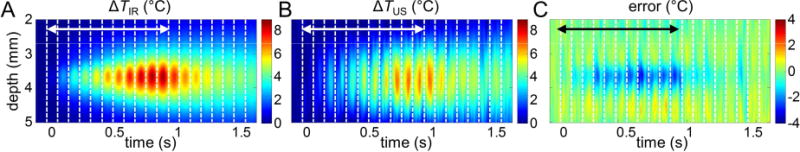
Evaluation of ultrasound temperature estimation: one tissue-mimicking phantom dataset. (A) The spatiotemporal evolution of temperature rise ΔT_IR measured by IR imaging. (B) The ultrasound estimated temperature rise ΔT_US. (C) Error = ΔT_US − ΔT_IR. The double-sided arrows indicate the time when HIFU is on.

Figure 7.

Error as a function of size of heating zone and ΔT_IR with error color-coded from (A) tissue-mimicking and (B) fat-mimicking phantom datasets.

Experiments using tissue specimens

We conducted experiments using cardiac tissue specimens with temperatures ranging from 20 to 100 °C to represent the scenarios in thermal ablation.

Ultrasound thermometry calibration

The spatiotemporal evolution of ΔT_IR (Fig. 8A) in the tissue specimen shows that during HIFU exposures, both the temperature and the size of the heated region increase as expected. The corresponding cum[ΔT_IR] and normalized ultrasound echo time shifts δτ′(y) are shown in Fig. 8B and Fig. 8C, respectively. To better illustrate the spatiotemporal changes, ΔT_IR, a, and R²_a,b as a function of time at the center focus, 0.2 mm and 0.4 mm away from the focus, are shown in Figs. 8D – F (locations indicated by white crosses in the first image in Fig. 8A). Compared with the phantom experiments, R²_a,b reaches above 0.75 much sooner, just after 0.2 s, as the temperature increased much faster in the tissue specimens (Fig. 8F), while the calibration parameter a becomes more stable only after the HIFUexposure (Fig. 8E). We determined, based on the fitting results with R²_a,b ≥ 0.75 from all A-lines in all frames (n = 15 sets of experiments, total of 22873 data points), that a = − 0.69 ± 0.18 (°C-mm/ns) for the tissue specimens.

Figure 8.

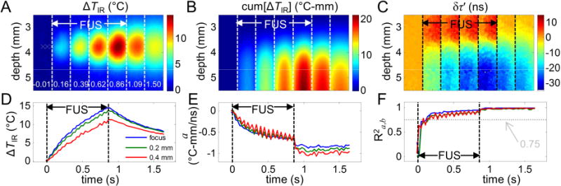
Example of calibration for porcine cardiac tissue: (A) 2D temperature rise ΔT_IR before, during, and after HIFU heating. The time is indicated in white numbers at the bottom of each frame in sec. (B) and (C) show the corresponding cum[ΔT_IR] and δτ′(y) = δτ(y) − δτ(y₀). (D) ΔT_IR as a function of time at the center focus, 0.2 mm and 0.4 mm away from the focus (locations indicated by white crosses in (A)). (E) and (F) show the corresponding fitted a and R²_a,b.

If we examine the results of calibration coefficient a against their corresponding max[ΔT_IR] at a 2 °C step (Fig. 9), we found that a was relatively constant with a gradual decrease (− 0.0074 °C-mm/ns per °C) during the range of temperature rise from 4 to 25 °C (corresponding to temperature 24 to 45 °C). However, a became more negative at larger temperature-rises above 25 °C, assumed larger absolute values, suggesting likely the nonlinearity of the temperature dependence of ultrasound echo time shifts. On the other hand, at small temperature increases (< 4 °C), the heating volume may not be large enough for accurate measurements and calibration.

Figure 9.

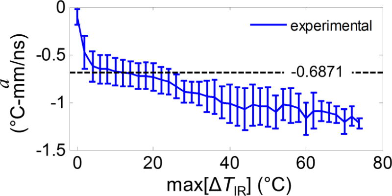
Calibrated coefficient a as a function of max[ΔT_IR] from 20 °C room temperature. The calibrated single value − 0.6871 is also shown in a dashed black line.

Evaluation of temperature estimation in ultrasound thermography

Figure 10 shows an example of the spatiotemporal evolution of ΔT_IR and ΔT_US and the corresponding error ΔT_US − ΔT_IR. Clearly, the error grows as temperature increases (Fig. 10C), which is further illustrated by the mean estimation error as a function of ΔT_IR and the size of the heating zone computed from all datasets (Fig. 11). It is seen that the temperature is underestimated with large temperature-rises (e.g. when ΔT_IR > 40 °C) and small heating region (e.g. < 2 mm) using ultrasound thermography. A largest error of − 40.1 °C was observed in a 1.25 mm heating zone at ΔT_IR = 68 °C.

Figure 10.

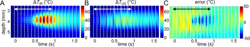
Evaluation of ultrasound temperature estimation: one porcine cardiac tissue dataset. (A) The spatiotemporal evolution of temperature rise ΔT_IR measured by IR imaging. (B) The ultrasound estimated temperature rise ΔT_US. (C) Error = ΔT_US − ΔT_IR. The double-sided arrows indicate the time when HIFU is on.

Figure 11.

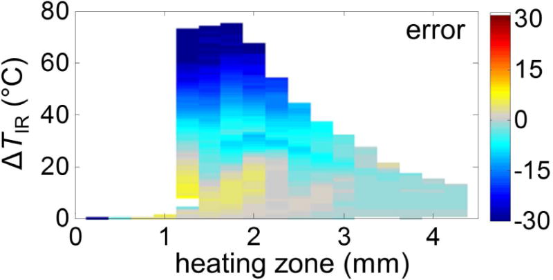
Error as a function of size of heating zone and ΔT_IR with error color-coded from the porcine cardiac tissue datasets.

DISCUSSION

We have investigated the applicability of IR thermography for evaluating ultrasound thermometry using HIFU as the heating modality.

We first derived a general expression for the echo time shifts accounting for isotropic free expansion of tissue during heating, and yielded an identical equation for gradient of echo time shift (Eq. 6) as derived by Simon et al. (1998). Echo time shift of ultrasound backscattered signals has not only been used for temperature estimation, but also applied to measure tissue properties such as thermal diffusivity by utilizing the bio-heat transfer equation (Anand and Kaczkowski 2008). In our derivations, the condition that a scatterer can move towards the transducer has also been discussed in Maass-Moreno and Damianou’s study (1996), given that the volume of tissue can move freely and thermal expansion is isotropic. The scatterer will not reach the transducer surface if there is sufficient fluid medium between the transducer and the specimen. However, if the specimen is in direct contact with the transducer, its movement should be limited by the transducer surface.

The assumption made for negligible effect of transducer self-heating in Eq. 1 holds with our experimental set-up. First, the medium between the transducer and the specimen was agar gel, which consisted mainly of water and a small amount of acoustic gel was also applied at the transducer surface to ensure good coupling. Secondly, the total imaging time for each individual experiment was only 1.8 sec (including pre-, during-, and post-HIFU application). Due to the short imaging time frame and the water-based medium which has a low thermal diffusivity, the temperature rise from the transducer itself has negligible effect on the ultrasound imaging. However, for experiments where the imaging probe is directly in contact with the specimen or where longer imaging time is required, the equations need to be re-derived to consider the effect of transducer self-heating on ultrasound thermometry.

Our uniquely constructed experimental setup allowed spatiotemporally correlated IR and ultrasound imaging to obtain measurement of HIFU-induced temperatures. After first obtaining material-dependent calibration coefficient, we then used the calibrated coefficient to estimate temperature through cross-validation of ultrasound signals and compute the estimation error by comparing the estimated temperatures against the IR measured temperatures. Our results in this study demonstrate the roles of several important factors affecting estimation of temperature using ultrasound thermography.

Geng et al. (2014) used IR thermography to compare with temperature measurements from ultrasound imaging during radio-frequency ablation (RFA). However, the lack of accurate tissue specific properties including IR emissivity and sound speed could introduce temperature estimation errors in both IR and ultrasound thermography. Also, the size of the heating volume from RFA is typically much larger than HIFU heating and hence their observations may not be directly applicable to a more localized heating using HIFU as illustrated by our results. Below, we further discuss the relevance of the factors we identified in ultrasound thermography calibration and evaluation.

Calibration of ultrasound thermometry using IR imaging and HIFU application

All methods of signal processing used for ultrasound thermometry require accurate calibration for the specific specimen for absolute and accurate temperature estimation (Arthur et al. 2005). For example, in the echo time shifts method used in this study, the knowledge of the material dependent calibration coefficient k (= 2a/c₀) is needed. In methods using the change of backscattered energy (CBE), it is necessary to know how backscattered energy changes as a function of temperature for a specific type of specimen (Arthur et al. 2010). Water-bath heating can be used to provide a controlled temperature environment for calibration. Although a smaller standard deviation and/or error may be possible because of the larger heated volume, a long time is often required for the water and sample to reach temperature equilibrium. In contrast, the calibration method we proposed using IR thermography with HIFU exposures can be performed within a relatively short period of time, in the order of just a few seconds.

However, as shown in this study, the small focal zone of HIFU transducer could result in small cumulative temperature increases thus small echo time shifts (e.g., Fig. 3F), making the analysis susceptive to noise in the cases with small heating volumes, although this can be relatively easily alleviated. As shown in our study, more accurate calibration was obtained with an increased region of temperature-rise, especially evident after HIFU was turned off and thermal conduction spread the temperature spatially.

It was also observed that larger propagation depth resulted in more noise in estimation of δτ due to the reduced ultrasound signal amplitude resulted from attenuation. Therefore for calibration we have only used data points within the center heating zone (0.2 × max[ΔT_IR]) to minimize errors. Susceptibility to noise may be a limiting factor for ultrasound thermometry in cases with low signal-to-noise ratios.

We assumed that the speed of sound changes linearly as a function of temperature (Eq. 5) in order to integrate ΔT_IR along the axial depth in our calibration. This assumption was shown to be valid in our phantom experiments, as demonstrated by the linear dependence of the calibrated a value on temperature up to 40 °C (e.g., Figs. 4D and 4E). However the linear assumption seems to be less applicable in the tissue experiments, since the calibrated a not only dropped to a more negative value at higher temperatures above 45 °C, a gradual decrease was also observed from 24 to 45 °C. Figure 9 (baseline temperature at 20 °C) implies that as the change of temperature exceeds 45 – 50 °C, the change in sound speed slows down, causing the echo time shift to further deviate from the linear relationship, leading to larger absolute values for a. In future studies, instead of a linear assumption, a quadratic relation (Miller et al. 2002) can also be assumed and further calibrated using the simultaneous ultrasound and IR imaging platform. If the precise relation between temperature changes and calibration coefficients, such as a, can be determined in advance, it may be possible to measure temperatures more accurately by applying different calibration values based on the estimated temperature at a previous time point.

The speed of sound and thermal expansion in most soft tissue (water-based) increase with increasing temperature, whereas in fat (lipid-based) they decrease as temperature increases (Bamber 2004; Duck 1990). These properties are consistent with the echo time shifts observed in the phantom experiments (Figs. 3C, 3F, 4C, 5A – D). One of the main difficulties to apply ultrasound thermometry in a clinical setting is the uncertainty of tissue content, and in vivo calibration of ultrasound thermography is generally unavailable. In vivo temperature measurement using MRI also suffers the same limitation where the unreliable temperature measurement in fat still remains a challenge (Rieke and Butts Pauly 2008). Thus IR thermography may be helpful in providing calibration on various different tissue types in a fast and systematic manner by establishing a database of the calibration coefficient for each tissue type. Although the platform proposed in this study cannot be directly applied to in vivo situations due to the limited penetration depth of IR thermography, newer platforms may be developed based on laparoscopic IR systems, which have been used in assessing tissue necrosis during radiofrequency ablation (Ogan et al. 2003) and in identifying anatomic and physical details during surgical procedures (Cadeddu et al. 2001; Song et al. 2009).

Validation of ultrasound thermometry using IR imaging

We choose cross-correlation to determine echo time shifts for ultrasound thermometry in this study. This method is inherently restricted to a temperature range in which change of speed of sound and thermal expansion are linearly dependent on temperature. Thus it is not surprising that ultrasound thermography in this study underestimated the temperatures at high temperatures when the linear relationship was no longer accurate. However, even in the linear range (e.g. Fig. 7), we observed that the estimation error of ultrasound thermography is closely related to the size of the heating volume. As shown in Figs. 5E – F, at a similar max[ΔT_IR], temperature estimation has a much smaller error with a larger heating zone, for example after HIFU was off, and with a higher R²_a,b (Fig. 4F).

In previous studies, polynomials with an order between 8 and 14 were used to fit the echo time shift δτ (Seip et al. 1996). In this study, δτ was fitted using a 10^th order polynomial. Taking the gradient of the polynomial can be considered equivalent to applying a narrowband differentiator directly to δτ. In a previous work (Simon et al. 1998), it was found that a better spatial resolution of temperature estimation from δτ was observed when a broadband differentiator was applied with the trade-off of increased amount of ripples. However, due to the small focal zone and small CNR in our experiments, we did not use broadband differentiators. As a result, the temperature-rise was underestimated within the focal zone during HIFU exposure. Oscillatory behaviors associated with differentiating high-order polynomials are also observed (Figs 5E – 5H). More advanced signal processing methods such as those using special filter designs can be employed (Ye et al. 2010) to minimize noise and further improve performance.

In previous ultrasound thermometry studies based on echo time shifts, good agreement of temperature estimation and thermocouple measurement (~0.5 °C) was achieved when the focal region was on the order of several millimeter to centimeter scale (Anand et al. 2007; Liu and Ebbini 2010; Seip et al. 1996; Simon et al. 1998). This study used sub-millimeter focal zone, as shown in Fig. 5A, which resulted in small CNR of δτ. Thus a slight difference between the slope of the fitted polynomial δτ and that of the δτ_IR in the focal zone results in a big difference in ΔT, suggesting that the size of the heating zone may limit the region where temperature can be precisely estimated using ultrasound thermography. As demonstrated in this study, IR imaging with high spatial resolution can be applied to readily evaluate the performance of ultrasound thermometry with varying size of heating zone. In contrast, thermocouples will be limited and insufficient to provide temperature information with a sub-millimeter spatial resolution.

System design and limitations

In this study, the duration of HIFU exposure was limited by the memory buffer on the digital oscilloscope which stores the ultrasound RF data. Due to this constraint, varying HIFU intensities were applied to generate different temperature increase in the same period of time. Therefore higher HIFU intensities were used in cardiac tissue experiments as compared to the phantom experiments to study tissue coagulation. If there were no memory buffer limitation, it would be interesting to study the effect of HIFU duration on the accuracy of ultrasound thermometry.

In addition, ultrasound imaging was performed with a 30 MHz center frequency transducer, and digitized at 500 Msample/s. Most ultrasound thermometry processing methods rely on changes in ultrasound signal due to temperature changes, therefore when the HIFU-generated spatial temperature gradient is very steep, a low frequency transducer might not have sufficient spatial resolution to detect the changes. Since clinical ultrasound transducers are often in the 1 – 20 MHz range, to achieve high accuracy in both calibration of tissue properties and temperature estimation, one can select a HIFU transducer with a larger focal volume or design a HIFU exposure sequence to avoid generating a steep spatial temperature gradient. The system design parameters can be optimized using the proposed platform.

The IR camera used in this study has a temperature measurement accuracy of ± 1 °C and a resolution of 0.01 °C, and the spatial resolution can reach 100 μm. When the camera price is considered, the optimal camera accuracy and resolution should be chosen based on the size of the HIFU generated temperature field. Since the HIFU transducers used in this study had small heating volumes (heating zones of only several millimeters), a high spatial resolution camera is required to record the complete temperature profile.

The penetration depth of the mid-infrared (3–5 μm) radiation in tissue is only 10–100 μm, which is mainly limited by the strong absorption of light by water molecules (Hale and Querry 1973). Therefore IR thermography measures an average temperature in a very thin slab close to the surface of the specimens. A direct comparison between the IR measurements with the ultrasound estimated temperature, which is strictly an average temperature through the slice thickness of the ultrasound imaging transducer, was possible because the high frequency ultrasound transducer used in this study has a lateral resolution of only 115 μm, comparable to the IR imaging slab. However, when an ultrasound imaging system with a lower lateral resolution is used, the temperature distribution at varying depths from the specimen surface needs to be considered, particularly the effects from wave interference and thermal conduction at the air-specimen interface. A potential way to calculate the average temperature in the same slice thickness as imaged by the ultrasound transducer is to reconstruct the temperature changes in the 3D subsurface volume through solving the inverse problem of bio-heat equations (Yin et al. 2013).

Other sources of error in temperature measurements

Ultrasound thermography is based on pulse-echo ultrasound interrogation, thus only 1D changes along the ultrasound line-of-sight are detected and used for estimation of temperature changes although 2D and 3D estimation can be obtained by raster scanning of the 1D ultrasound interrogation beam. As such, the expression derived by Simon et al. (Simon et al. 1998) and our expression in Eq. 3 of the echo time shift detection relies on the 1D nature of pulse-echo imaging. While this assumption has no bearing on the signal change associated with the temperature-depended change of sound speed, it affects the detection of 3D thermal expansion. Since each A-line of pulse-echo ultrasound only detects the projection of the 3D expansion along the line of sight of ultrasound beam, errors in temperature estimation arise particularly in a small heating volume or in regions far from the center of heating laterally.

In addition, the accuracy of IR thermography for temperature measurement is highly dependent on the accuracy of emissivity measurement. The background temperature also needs to be precisely measured to subtract its effect (Öhman 2001). In this study, the maximum error in IR temperature measurement due to emissivity error (± 0.03) is small (around ± 0.5 °C) for emissivity ranging from 0.87 – 0.99 for the phantoms and cardiac tissue specimens. However, when the specimen of interest has a much lower emissivity (e.g., < 0.5), care must be taken because temperature conversion from IR radiation is more sensitive to emissivity error for low emissivity specimens. The black-tape method applied in this study is the simplest and most cost-down way for emissivity measurement. The measurement error using this method has been investigated in detail (Madding 2003) and it is recommended that the object of interest is raised 20 °C or more above the background temperature for accurate measurement. In this study, the room temperature was kept at 20 °C so the experiments were performed at around 40 °C. However, the method is no longer applicable if the background temperature is higher and potential thermal damage may alter the tissue properties. Sanchez-Marin et al.’s (2009) proposed method for measuring emissivity of the human skin using infrared camera and CO₂ laser beam may be a suitable alternative for tissue emissivity measurement. Unlike traditional methods, it does not require absolute temperature information so a blackbody or a reference temperature sensor is not required.

CONCLUSIONS

In this study, we show the utility of IR imaging/thermography for fast calibration and validation of signal processing algorithms in ultrasound thermography. Using simultaneous and correlated ultrasound and IR imaging, we demonstrated the procedures and identified the factors involved in the calibration and evaluation of ultrasound thermography. High resolution of IR imaging also facilitates evaluation of spatial resolution of ultrasound thermography. Although in this study HIFU was chosen as the heat source and echo time shifts were for ultrasound signals, the methodology described in this study has the potential to help the development of ultrasound thermometry for other types of thermal therapies and data processing methods.

References

- Amini AN, Ebbini ES, Georgiou TT. Noninvasive estimation of tissue temperature via high-resolution spectral analysis techniques. IEEE Trans Biomed Eng. 2005;52(2):221–228. doi: 10.1109/TBME.2004.840189. [DOI] [PubMed] [Google Scholar]
- Anand A, Kaczkowski PJ. Noninvasive measurement of local thermal diffusivity using backscattered ultrasound and focused ultrasound heating. Ultrasound Med Biol. 2008;34(9):1449–1464. doi: 10.1016/j.ultrasmedbio.2008.02.004. [DOI] [PMC free article] [PubMed] [Google Scholar]
- Anand A, Savery D, Hall C. Three-dimensional spatial and temporal temperature imaging in gel phantoms using backscattered ultrasound. IEEE Trans Ultrason Ferroelectr Freq Control. 2007;54(1):23–31. doi: 10.1109/tuffc.2007.208. [DOI] [PubMed] [Google Scholar]
- Arthur RM, Basu D, Guo YZ, Trobaugh JW, Moros EG. 3-D in vitro estimation of temperature using the change in backscattered ultrasonic energy. IEEE Trans Ultrason Ferroelectr Freq Control. 2010;57(8):1724–1733. doi: 10.1109/TUFFC.2010.1611. [DOI] [PubMed] [Google Scholar]
- Arthur RM, Straube WL, Trobaugh JW, Moros EG. Non-invasive estimation of hyperthermia temperatures with ultrasound. Int J Hyperthermia. 2005;21(6):589–600. doi: 10.1080/02656730500159103. [DOI] [PubMed] [Google Scholar]
- Bamber JC. Speed of sound. In: Hill CR, Bamber JC, ter Haar GR, editors. Physical principles of medical ultrasonics. 2nd. Chicester, West Sussex, England: John Wiley & Sons, Ltd; 2004. pp. 167–190. [Google Scholar]
- Bobkova S, Gavrilov L, Khokhlova V, Shaw A, Hand J. Focusing of high-intensity ultrasound through the rib cage using a therapeutic random phased array. Ultrasound Med Biol. 2010;36(6):888–906. doi: 10.1016/j.ultrasmedbio.2010.03.007. [DOI] [PMC free article] [PubMed] [Google Scholar]
- Cadeddu JA, Jackman SV, Schulam PG. Laparoscopic infrared imaging. J Endourol. 2001;15:111–116. doi: 10.1089/08927790150501033. [DOI] [PubMed] [Google Scholar]
- Clarke RL, ter Haar GR. Temperature rise recorded during lesion formation by high-intensity focused ultrasound. Ultrasound Med Biol. 1997;23(2):299–306. doi: 10.1016/s0301-5629(96)00198-6. [DOI] [PubMed] [Google Scholar]
- Crouzet S, Murat FJ, Pasticier G, Cassier P, Chapelon JY, Gelet A. High intensity focused ultrasound (HIFU) for prostate cancer: Current clinical status, outcomes and future perspectives. Int J Hyperthermia. 2010;26(8):796–803. doi: 10.3109/02656736.2010.498803. [DOI] [PubMed] [Google Scholar]
- Dewhirst MW, Prosnitz L, Thrall D, Prescott D, Clegg S, Charles C, MacFall J, Rosner G, Samulski T, Gillette E, LaRue S. Hyperthermic treatment of malignant diseases: current status and a view toward the future. Semin Oncol. 1997;24(6):616–625. [PubMed] [Google Scholar]
- Diakides NA, Diakides M, Lupo JC, Paul JL, Balcerak R. Advances in medical infrared imaging. In: Diakides NA, Bronzino JD, editors. Medical Infrared Imaging. New York, NY: CRC Press; 2008. pp. 1-1–1-13. [Google Scholar]
- Duck FA. Physical Properties of Tissue. Academic Press Inc; 1990. [Google Scholar]
- Franckena M, Lutgens LC, Koper PC, Kleynen CE, van der Steen-Banasik EM, Jobsen JJ, Leer JW, Creutzberg CL, Dielwart MF, van Norden Y, Canters RA, van Rhoon GC, van der Zee J. Radiotherapy and hyperthermia for treatment of primary locally advanced cervix cancer: results in 378 patients. Int J Radiat Oncol Biol Phys. 2009;73(1):242–250. doi: 10.1016/j.ijrobp.2008.03.072. [DOI] [PubMed] [Google Scholar]
- Fry WJ, Fry RB. Determination of absolute sound levels and acoustic absorption coefficients by thermocouple probes – theory. J Acoust Soc Am. 1954;26(3):294–310. [Google Scholar]
- Geng X, Zhou Z, Li Q, Wu S, Wang C-Y, Liu H-L, Chuang C-C, Tsui P-H. Comparison of ultrasound temperature imaging with infrared thermometry during radio frequency ablation. Jpn J Appl Phys. 2014;53:047001. [Google Scholar]
- Giridhar D, Robinson RA, Liu Y, Sliwa J, Zderic V, Myers MR. Quantitative estimation of ultrasound beam intensities using infrared thermography—Experimental validation. J Acoust Soc Am. 2012;131(6):4283–4291. doi: 10.1121/1.4711006. [DOI] [PubMed] [Google Scholar]
- Goldberg SN, Gazelle GS, Mueller PR. Thermal ablation therapy for focal malignancy: a unified approach to underlying principles, techniques, and diagnostic imaging guidance. Am J Roentgenol. 2000;174(2):323–331. doi: 10.2214/ajr.174.2.1740323. [DOI] [PubMed] [Google Scholar]
- Hale GM, Querry MR. Optical constants of water in the 200-nm to 200-μm wavelength region. Appl Opt. 1973;12(3):555–563. doi: 10.1364/AO.12.000555. [DOI] [PubMed] [Google Scholar]
- Hand JW, Shaw A, Sadhoo N, Rajagopal S, Dickinson RJ, Gavrilov LR. A random phased array device for delivery of high intensity focused ultrasound. Phys Med Biol. 2009;54(19):5675–5693. doi: 10.1088/0031-9155/54/19/002. [DOI] [PubMed] [Google Scholar]
- Hsiao Y-S, Kumon RE, Deng CX. Characterization of lesion formation and bubble activities during high-intensity focused ultrasound ablation using temperature-derived parameters. Infrared Phys Techn. 2013;60:108–117. doi: 10.1016/j.infrared.2013.04.002. [DOI] [PMC free article] [PubMed] [Google Scholar]
- Incropera FP, Dewitt DP, Bergman TL, Lavine AS. Introduction to heat transfer. 5th. Hoboken, NJ: John Wiley & Sons, Inc; 2007. Radiation: processes and properties. [Google Scholar]
- Jolesz FA. MRI-guided focused ultrasound surgery. Annu Rev Med. 2009;60:417–430. doi: 10.1146/annurev.med.60.041707.170303. [DOI] [PMC free article] [PubMed] [Google Scholar]
- Kennedy JE. High-intensity focused ultrasound in the treatment of solid tumours. Nat Rev Cancer. 2005;5(4):321–327. doi: 10.1038/nrc1591. [DOI] [PubMed] [Google Scholar]
- Kopelman D, Inbar Y, Hanannel A, Freundlich D, Castel D, Perel A, Greenfeld A, Salamon T, Sareli M, Valeanu A, Papa M. Magnetic resonance-guided focused ultrasound surgery (MRgFUS): Ablation of liver tissue in a porcine model. Eur J Radiol. 2006;59(2):157–162. doi: 10.1016/j.ejrad.2006.04.008. [DOI] [PubMed] [Google Scholar]
- Liu D, Ebbini ES. Real-time 2-D temperature imaging using ultrasound. IEEE Trans Biomed Eng. 2010;57(1):12–16. doi: 10.1109/TBME.2009.2035103. [DOI] [PMC free article] [PubMed] [Google Scholar]
- Liu HL, Li ML, Shih TC, Huang SM, Lu IY, Lin DY, Lin SM, Ju KC. Instantaneous frequency-based ultrasonic temperature estimation during focused ultrasound thermal therapy. Ultrasound Med Biol. 2009;35(10):1647–1661. doi: 10.1016/j.ultrasmedbio.2009.05.004. [DOI] [PubMed] [Google Scholar]
- Maass-Moreno R, Damianou CA. Noninvasive temperature estimation in tissue via ultrasound echo-shifts. 1. Analytical model. J Acoust Soc Am. 1996;100(4):2514–2521. doi: 10.1121/1.417359. [DOI] [PubMed] [Google Scholar]
- Maass-Moreno R, Damianou CA, Sanghvi NT. Noninvasive temperature estimation in tissue via ultrasound echo-shifts. 2. In vitro study. J Acoust Soc Am. 1996;100(4):2522–2530. doi: 10.1121/1.417360. [DOI] [PubMed] [Google Scholar]
- Madding RP. Emissivity measurement using infrared imaging radiometric cameras. In: Driggers RG, editor. Encyclopedia of optical engineering. Vol. 2. New York, NY: CRC Press; 2003. pp. 475–483. [Google Scholar]
- Madsen EL, Zagzebski JA, Banjavie RA, Jutila RE. Tissue mimicking materials for ultrasound phantoms. Med Phys. 1978;5(5):391–394. doi: 10.1118/1.594483. [DOI] [PubMed] [Google Scholar]
- Madsen EL, Zagzebski JA, Frank GR. Oil-in-gelatin dispersions for use as ultrasonically tissue-mimicking materials. Ultrasound Med Biol. 1982;8(3):277–287. doi: 10.1016/0301-5629(82)90034-5. [DOI] [PubMed] [Google Scholar]
- Miller NR, Bamber JC, Meaney PM. Fundamental limitations of noninvasive temperature imaging by means of ultrasound echo strain estimation. Ultrasound Med Biol. 2002;28(10):1319–1333. doi: 10.1016/s0301-5629(02)00608-7. [DOI] [PubMed] [Google Scholar]
- Morris H, Rivens I, Shaw A, ter Haar G. Investigation of the viscous heating artefact arising from the use of thermocouples in a focused ultrasound field. Phys Med Biol. 2008;53(17):4759–4776. doi: 10.1088/0031-9155/53/17/020. [DOI] [PubMed] [Google Scholar]
- Myers MR, Giridhar D. Theoretical framework for quantitatively estimating ultrasound beam intensities using infrared thermography. J Acoust Soc Am. 2011;129(6):4073–4083. doi: 10.1121/1.3575600. [DOI] [PubMed] [Google Scholar]
- Ogan K, Roberts WW, Wilhelm DM, Bonnell L, Leiner D, Lindberg G, Kavoussi LR, Cadeddu JA. Infrared thermography and thermocouple mapping of radiofrequency renal ablation to assess treatment adequacy and ablation margins. Urology. 2003;62(1):146–151. doi: 10.1016/s0090-4295(03)00040-2. [DOI] [PubMed] [Google Scholar]
- Öhman C. Measurement in thermography. FLIR Systems AB. 2001:22–35. [Google Scholar]
- Owen NR, Chapelon JY, Bouchoux G, Berriet R, Fleury G, Lafon C. Dual-mode transducers for ultrasound imaging and thermal therapy. Ultrasonics. 2010;50(2):216–220. doi: 10.1016/j.ultras.2009.08.009. [DOI] [PubMed] [Google Scholar]
- Patel P, Luk A, Durrani A, Dromi S, Cuesta J, Angstadt M, Dreher M, Wood B, Frenkel V. In vitro and in vivo evaluations of increased effective beam width for heat deposition using a split focus high intensity ultrasound (HIFU) transducer. Int J Hyperthermia. 2008;24(7):537–549. doi: 10.1080/02656730802064621. [DOI] [PMC free article] [PubMed] [Google Scholar]
- Qiu Z, Gao J, Cochran S, Huang ZH, Corner G, Song CL. The development of therapeutic ultrasound with assistance of robotic manipulator. Proc 35th Annual Intl Conf IEEE Engin Med Biol Soc: IEEE. 2009:733–736. doi: 10.1109/IEMBS.2009.5332414. [DOI] [PubMed] [Google Scholar]
- Rieke V, Butts Pauly K. MR thermometry. J Magn Reson Imaging. 2008;27(2):376–390. doi: 10.1002/jmri.21265. [DOI] [PMC free article] [PubMed] [Google Scholar]
- Rivens I, Shaw A, Civale J, Morris H. Treatment monitoring and thermometry for therapeutic focused ultrasound. Int J Hyperthermia. 2007;23(2):121–139. doi: 10.1080/02656730701207842. [DOI] [PubMed] [Google Scholar]
- Ryu KS, Kim JH, Ko HS, Kim JW, Ahn WS, Park YG, Kim SJ, Lee JM. Effects of intraperitoneal hyperthermic chemotherapy in ovarian cancer. Gynecol Oncol. 2004;94(2):325–332. doi: 10.1016/j.ygyno.2004.05.044. [DOI] [PubMed] [Google Scholar]
- Sanchez-Marin FJ, Calixto-Carrera S, Villaseñor-Mora C. Novel approach to assess the emissivity of the human skin. J Biomed Opt. 2009;14(2):024006. doi: 10.1117/1.3086612. [DOI] [PubMed] [Google Scholar]
- Seip R, VanBaren P, Cain CA, Ebbini ES. Noninvasive real-time multipoint temperature control for ultrasound phased array treatments. IEEE Trans Ultrason Ferroelectr Freq Control. 1996;43(6):1063–1073. [Google Scholar]
- Simon C, Vanbaren P, Ebbini ES. Two-dimensional temperature estimation using diagnostic ultrasound. IEEE Trans Ultrason Ferroelectr Freq Control. 1998;45(4):1088–1099. doi: 10.1109/58.710592. [DOI] [PubMed] [Google Scholar]
- Song C, Marshall B, McLean D, Frank TG, Sibbett W, Cuschieri A, Campbell PA. Thermographic investigation of the heating effect of high intensity focused ultrasound. Proc 27th Annual Intl Conf IEEE Engin Med Biol Soc: IEEE. 2005:3456–3458. doi: 10.1109/IEMBS.2005.1617222. [DOI] [PubMed] [Google Scholar]
- Song C, Tang B, Campbell PA, Cuschieri A. Thermal spread and heat absorbance differences between open and laparoscopic surgeries during energized dissections by electrosurgical instruments. Surg Endosc. 2009;23:2480–2487. doi: 10.1007/s00464-009-0421-7. [DOI] [PubMed] [Google Scholar]
- Staruch R, Chopra R, Hynynen K. Localised drug release using MRI-controlled focused ultrasound hyperthermia. Int J Hyperthermia. 2011;27(2):156–171. doi: 10.3109/02656736.2010.518198. [DOI] [PubMed] [Google Scholar]
- Straube WL, Arthur RM. Theoretical estimation of the temperature-dependence of backscattered ultrasonic power for noninvasive thermometry. Ultrasound Med Biol. 1994;20(9):915–922. doi: 10.1016/0301-5629(94)90051-5. [DOI] [PubMed] [Google Scholar]
- Tsui PH, Chien YT, Liu HL, Shu YC, Chen WS. Using ultrasound CBE imaging without echo shift compensation for temperature estimation. Ultrasonics. 2012a;52(7):925–935. doi: 10.1016/j.ultras.2012.03.001. [DOI] [PubMed] [Google Scholar]
- Tsui PH, Shu YC, Chen WS, Liu HL, Hsiao IT, Chien YT. Ultrasound temperature estimation based on probability variation of backscatter data. Med Phys. 2012b;39(5):2369–2385. doi: 10.1118/1.3700235. [DOI] [PubMed] [Google Scholar]
- Varghese T, Zagzebski JA, Chen Q, Techavipoo U, Frank G, Johnson C, Wright A, Lee FT. Ultrasound monitoring of temperature change during radiofrequency ablation: preliminary in-vivo results. Ultrasound Med Biol. 2002;28(3):321–329. doi: 10.1016/s0301-5629(01)00519-1. [DOI] [PubMed] [Google Scholar]
- Wu F. Extracorporeal high intensity focused ultrasound in the treatment of patients with solid malignancy. Minim Invasiv Ther. 2006;15(1):26–35. doi: 10.1080/13645700500470124. [DOI] [PubMed] [Google Scholar]
- Ye GL, Smith PP, Noble JA. Model-based ultrasound temperature visualization during and following HIFU Exposure. Ultrasound Med Biol. 2010;36(2):234–249. doi: 10.1016/j.ultrasmedbio.2009.10.001. [DOI] [PubMed] [Google Scholar]
- Yin L, Gudur MSR, Hsiao Y-S, Kumon RE, Deng CX, Jiang H. Tomographic reconstruction of tissue properties and temperature increase for high-intensity focused ultrasound applications. Ultrasound Med Biol. 2013;39(10):1760–1770. doi: 10.1016/j.ultrasmedbio.2013.04.009. [DOI] [PMC free article] [PubMed] [Google Scholar]
- Zagar TM, Oleson JR, Vujaskovic Z, Dewhirst MW, Craciunescu OI, Blackwell KL, Prosnitz LR, Jones EL. Hyperthermia combined with radiation therapy for superficial breast cancer and chest wall recurrence: a review of the randomised data. Int J Hyperthermia. 2010;26(7):612–617. doi: 10.3109/02656736.2010.487194. [DOI] [PMC free article] [PubMed] [Google Scholar]