Automated segmentation of dental CBCT image with prior-guided sequential random forests

Abstract

Purpose:

Cone-beam computed tomography (CBCT) is an increasingly utilized imaging modality for the diagnosis and treatment planning of the patients with craniomaxillofacial (CMF) deformities. Accurate segmentation of CBCT image is an essential step to generate 3D models for the diagnosis and treatment planning of the patients with CMF deformities. However, due to the image artifacts caused by beam hardening, imaging noise, inhomogeneity, truncation, and maximal intercuspation, it is difficult to segment the CBCT.

Methods:

In this paper, the authors present a new automatic segmentation method to address these problems. Specifically, the authors first employ a majority voting method to estimate the initial segmentation probability maps of both mandible and maxilla based on multiple aligned expert-segmented CBCT images. These probability maps provide an important prior guidance for CBCT segmentation. The authors then extract both the appearance features from CBCTs and the context features from the initial probability maps to train the first-layer of random forest classifier that can select discriminative features for segmentation. Based on the first-layer of trained classifier, the probability maps are updated, which will be employed to further train the next layer of random forest classifier. By iteratively training the subsequent random forest classifier using both the original CBCT features and the updated segmentation probability maps, a sequence of classifiers can be derived for accurate segmentation of CBCT images.

Results:

Segmentation results on CBCTs of 30 subjects were both quantitatively and qualitatively validated based on manually labeled ground truth. The average Dice ratios of mandible and maxilla by the authors’ method were 0.94 and 0.91, respectively, which are significantly better than the state-of-the-art method based on sparse representation (p-value < 0.001).

Conclusions:

The authors have developed and validated a novel fully automated method for CBCT segmentation.

1. INTRODUCTION

Craniomaxillofacial (CMF) deformities involve congenital and acquired deformities of head and face. The number of patients with acquired deformity is large. In the last decade, the cone-beam computed topography (CBCT) scan has become widely used as a valuable technique in diagnosis and treatment planning of patients with CMF deformities due to the lower radiation and lower cost, compared with the spiral multislice CT (MSCT) scan. To accurately assess CMF deformities and treatment planning, one critical step is to segment the CBCT image to generate a 3D model, which includes segmentation of bony structures from soft tissues, and separation of mandible from maxilla.¹ For the purpose of clear presentation, we refer “maxilla” as “the midface and the maxilla” in the following text. However, due to the image artifacts caused by beam hardening, imaging noise, inhomogeneity, and truncation, it is very difficult to segment the CBCT.² Moreover, in order to better quantify the deformities, CBCT scans are usually acquired when the maxillary (upper) and mandibular (lower) teeth are in maximal intercuspation (MI), which brings even more challenges to separate the mandible from the maxilla.³

To date, there is limited work that could effectively segment both maxilla and mandible from CBCT. Manual segmentation is tedious, time-consuming, and user-dependent. It usually takes 5–6 h to segment the maxillomandibular region.⁴ Previous automated segmentation methods are mainly based on thresholding and morphological operations,⁵ which are sensitive to the presence of the artifacts.⁶ Recently, shape information has been utilized for robust segmentation.^7–12 Duy et al.,¹⁰ proposed a novel statistical shape model for detection and classification of teeth in CBCTs. However, their method may not be able to handle pathological cases, where shapes often change significantly (as shown by examples in the Sec. 3). This is because their method relies on a shape prior, which is easy to obtain for normal subjects, but difficult for pathological subjects. Inspired by the multiatlas label fusion work,^13–18 Wang et al.,² proposed a novel patch-based sparse labeling method for automated segmentation of CBCT images. However, it is computationally expensive (taking hours) due to (1) the requirement of nonlinear registrations between multiple atlases and the target image and (2) patch-based sparse representation (SR)^19–21 for each voxel. Moreover, if a larger number of atlases are used, the computational time becomes even longer. Another limitation is that only simple intensity patches are employed as features to guide the segmentation, which may further limit its performance.

Recently, random forest^22–27 has attracted rapidly growing interest. It is a nonparametric method that builds an ensemble model of decision trees from random subsets of features and the bagged samples of the training data and has achieved state-of-the-art performance in many image-processing problems.^24,25,28 In this paper, we present a novel learning-based framework to simultaneously segment both maxilla and mandible from CBCT based on random forest. Our framework is able to integrate information from multisource images for accurate CBCT segmentation. Specifically, the multisource images used in our work include the original CBCT images and the iteratively refined probability maps for mandible and maxilla. As a learning-based approach, our framework consists of two stages: training stage and testing stage. (1) In the training stage, we first employ majority voting (MV) to estimate the initial segmentation probability maps of mandible and maxilla based on multiple aligned expert-segmented CBCT images. The initial probability maps provide a prior guidance for the segmentation.²³ We then extract both the appearance features from CBCTs and the context features from the estimated probability maps,^29,30 which are then used to refine the segmentations of mandible and maxilla with random forest that can select discriminative features for segmentation. By iteratively training the subsequent classifiers with random forest on both the original CBCT and the updated segmentation probability maps, we can train a sequence of classifiers for CBCT segmentation. (2) Similarly, in the testing stage, given a target image, the learned classifiers are sequentially applied to iteratively refine the probability maps by combining previous probability maps with the original CBCT image. We have validated the proposed work on 30 sets of CBCT images and additional 60 sets of MSCT images. Compared to the state-of-the-art segmentation methods, our method achieves more accurate results.

Compared with previous works,^24,25 our work differs in two aspects: (1) Instead of training a classifier by the training samples in each atlas, the proposed method trains a classifier using all training samples in all atlases. Although this will be computationally demanding, training a classifier by all training data often gives much better results.²⁴ (2) Compared with the standard random forest scheme, our method trains a sequence of classifiers, instead of one classifier, which could integrate neighboring label information for refining the classification results. It should be noted that similar work has been presented in Ref. 26, in which a sequence of random forest classifiers was used for infant brain segmentation. However, the spatial prior, which is important for segmentation,^23,24 was ignored in Ref. 26. In this paper, we propose to integrate spatial prior into classification-based segmentation, which shows much better performance than using image appearances alone. Besides, unlike most of existing methods,^24–26 which focus on only the brain images, our method aims to address the challenges in segmentation of CBCT maxilla and mandible.

2. METHOD

In this paper, we formulate the CBCT segmentation as a classification problem. Random forest²² is adopted in our approach as a multiclass classifier to produce probability maps for each class (i.e., maxilla, mandible, and background) by voxelwise classification. The final segmentation is accomplished by assigning the label with the largest probability at each voxel location. As a supervised learning method, our method has training and testing stages.

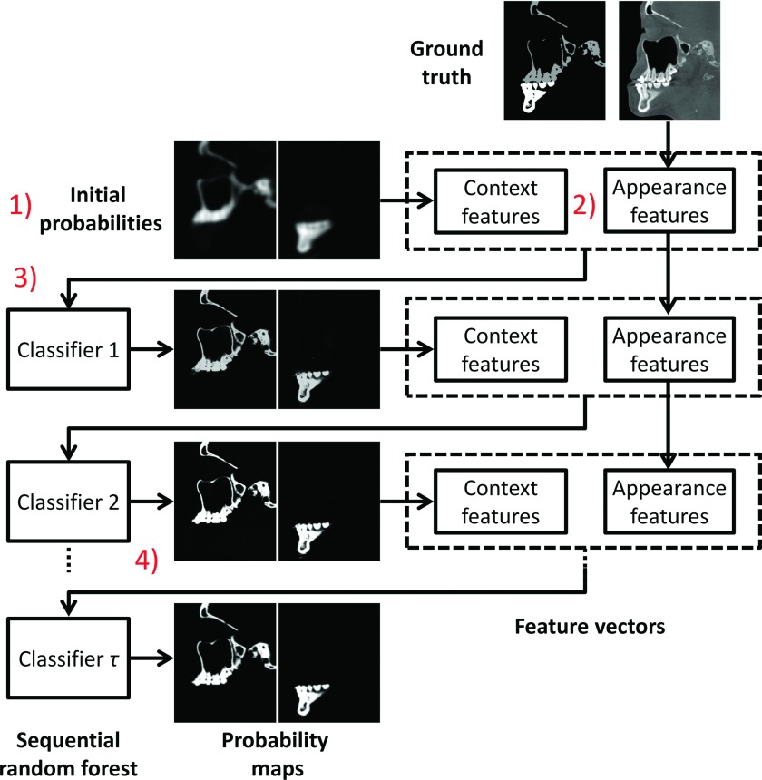
The flowchart of the training stage is shown in Fig. 1. In the training stage, (1) Majority voting is used to estimate the initial probability maps of mandible and maxilla according to a set of aligned expert-segmented CBCT scans that are used as multiatlases. (2) Both the appearance features and the context features are extracted from CBCT and the estimated segmentation probability maps, respectively. (3) The extracted features are used to refine the segmentations of mandible and maxilla with random forest that can select discriminative features for segmentation. (4) Based on the classifier trained in previous step, we can further update the segmentation probability maps. Similarly, based on the updated probability maps, we can further train the next classifier. This kind of procedure can be alternately performed to deal with challenges of image artifacts and maximal intercuspation (i.e., upper and lower teeth bite closely in MI during CBCT scanning—a clinical requirement for the purpose of accurately quantifying deformities). These four training steps are summarized in details below.

FIG. 1.

Flowchart of the proposed training steps using CBCT image, as well as maxilla and mandible probabilities. The appearance features from CBCT images and the context features from iteratively updated probability maps are integrated for training a sequence of classifiers.

Step 1: Estimation of initial probability maps with majority voting. In our approach, all the expert-segmented CBCT scans are used as training atlases and further aligned onto the subject CBCT image by affine registration. (Note that in our leave-one-out validation procedure, the testing CBCT image will be excluded for the estimation of initial probability maps.) Then, we employ majority voting to count the votes for each label for estimating the initial probability maps of both maxilla and mandible at every voxel, for their rough localizations. This simple approach has been proven very robust. The initial probability maps provide spatial priors which are important for guiding the segmentation.^23,24

Step 2: Extraction of CBCT appearance and context features. We extract these features for training classifiers. Specifically, we extract appearance features from CBCT, i.e., random Haar-like features.³¹ We also extract the context features from the previous segmentation probability maps. They are used to coordinate the segmentations in different parts of CBCT image. For the purpose of efficiency, we use the same Haar-like definition to extract context features. This context features has been shown effective in both computer vision and medical image analysis fields.^32–35 It is important to note that the extraction of context features is recursively conducted on the iteratively updated probability maps. This is different from the extraction of appearance features, which is performed on the original CBCT images.

Step 3: Training of random forest based classifiers. To refine the segmentations, we train a classifier to learn the complex relationship between local appearance/context features and the corresponding manual segmentation labels on all voxels of the training atlases. Although many advanced classifiers have been developed in the past, e.g., support vector machine (SVM),³⁶ random forest^22,27 is used in our approach, because of (1) its effectiveness in handling a large number of training data with high dimensionality and (2) its fast speed in testing (although slow in training). In addition, random forest also allows us to explore a large number of image features to select the most suitable ones for accurate CBCT segmentation.

Step 4: Repeating Steps 2 and 3 until convergence. In this final step, we train our classifiers in a sequential manner. Specifically, based on the classifier trained in Step 3, we update the segmentation probability maps. Then, according to Step 2, we extract the context features from the updated segmentation probability maps and further use with the original CBCT appearance features to train a next classifier. Eventually, we train and obtain a sequence of sequential classifiers for CBCT segmentation.

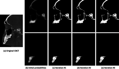
In the testing stage, given a new CBCT image, as shown in Fig. 2(a), the corresponding probability maps of the maxilla and the mandible can be estimated by using the sequentially trained classifiers. Specifically, as Step 1 of the training stage, the initial segmentation probability maps of the maxilla and the mandible are first estimated using majority voting [Fig. 2(b)]. Then, based on the estimated probability maps, the context features are extracted and, together with CBCT appearance features, served as the input to the sequential classifiers for iteratively updating the segmentation probability maps. Based on the output of the sequential classifiers, the new CBCT image is finally segmented. As shown in Figs. 2(b)–2(e), the probability maps are updated with the iterations, becoming more and more accurate.

FIG. 2.

The estimated probability maps by applying a sequence of trained classifiers on an unseen CBCT image (a). The probability maps become more accurate and sharper with the iterations [(b)–(e)].

2.A. Random forests

In this section, we will introduce the details of random forest to determine a class label c ∈ C for a given testing voxel x ∈ Ω, based on its high-dimensional feature representation $f\left(x,I\right)$, where I is a set consisting of CBCT intensity images and segmentation probability maps. The random forest is an ensemble of decision trees, indexed by $t\in \left[1,T\right]$, where T is the total number of trees at each iteration. A decision tree consists of two types of nodes, namely, internal nodes (nonleaf nodes) and leaf nodes. Each internal node stores a split (or decision) function, according to which the incoming data are sent to its left or right child node, and each leaf stores the final answer (predictor).²⁷ During training, each tree t learns a weak class predictor $p_t\left(c|f\left(x,I\right)\right)$. The training is performed by splitting the training voxels at each internal node based on their feature representations and further assigning samples to the left and right child nodes for recursive splitting. Specifically, at each internal node, to inject the randomness for improved generalization, a sampled subset Θ of all possible features is randomly selected.^27,37 A number of random splits on different combinations of feature and threshold is considered, and the one maximizing the information gain^25,27,37 is chosen as the optimal split. The tree continues to grow as more splits are made and stops at a specified depth (D), also with the condition that no tree leaf node contains less than a certain number of training samples $\left(s_{min}\right)$. Finally, by simply counting the labels of all training samples which reach each leaf node, we can associate each leaf node l with the empirical distribution over classes $p_t^l\left(c|f\left(x,I\right)\right)$.

During testing, each voxel x to be classified is independently pushed through each trained tree t, by applying the learned split functions. Upon arriving at a leaf node l_x, the empirical distribution of the leaf node is used to determine the class probability of the testing sample x at tree t, i.e., $p_t\left(c|f\left(x,I\right)\right)=p_t^{l_x}\left(c|f\left(x,I\right)\right)$. The final probability of the testing sample x is computed as the average of the class probabilities from individual trees, i.e., $p\left(c|x\right)=1/T{\sum }_{t=1}^T{p}_t\left(c|f\left(x,I\right)\right)$.

2.B. Appearance and context features

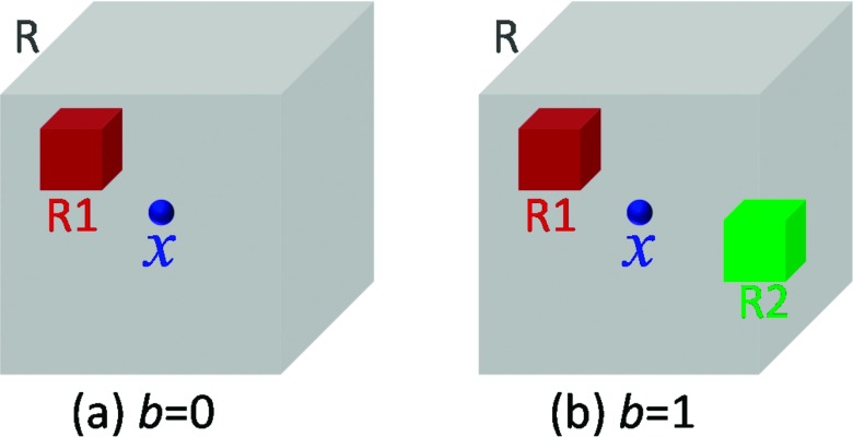
Although our framework can utilize any kind of features from original CBCT images and probability maps, such as SIFT,³⁸ HOG,³⁹ and LBP features,⁴⁰ for classification purpose, the 3D Haar-like features are used in our work due to computational efficiency. Specifically, for each voxel x in the original CBCT image or probability maps, its Haar-like features are computed as the local mean intensity of any randomly displaced cubical region R₁ [Fig. 3(a)], or the mean intensity difference over any two randomly displaced, asymmetric cubical regions (R₁ and R₂) [Fig. 3(b)], within a patch R,⁴¹

$${\displaystyle f\left(x,I\right)=\frac{1}{\left|R_1\right|}\sum _{u\in R_1}I\left(u\right)-b\frac{1}{\left|R_2\right|}\sum _{v\in R_2}I\left(v\right),R_1\in R,R_2\in R,b\in \left\{0,1\right\},}$$ (1)

where R is the patch centered at voxel x, I is an original CBCT image or a probability map, and the parameter $b\in \left\{0,1\right\}$ indicates whether one or two cubical regions are used, as shown in Figs. 3(a) and 3(b), respectively. In our work, appearance and context features are both Haar-like features. The only difference is that appearance features are extracted from CBCT image, while context features are extracted from probability maps. For a patch R in a CBCT image, its intensities are normalized with the unit ℓ2 norm^42,43 before extraction of Haar-like features. However, for a patch in a probability map, we did not perform any normalization.

FIG. 3.

Extraction of 3D Haar-like features. The gray cubic indicated a patch R centered at x. (a) If b = 0, a Haar-like feature is computed as the local mean intensity of any randomly displaced cubical region R₁ within the image patch R. (b) If b = 1, a Haar-like feature is computed as the mean intensity difference over any two randomly displaced, asymmetric cubical regions (R₁ and R₂) within the image patch R.

3. VALIDATION AND RESULTS

This study included the CBCT scans of 30 patients (12 males/18 females) with nonsyndromic dentofacial deformity, treated with a double-jaw orthognathic surgery. They were randomly selected from our clinical archive. The patient’s ages were 24 ± 10 yr (range: 10–49 yr). These CBCT scans were acquired in a CBCT scanner (i-CAT, Imaging Sciences International LLC, Hatfield, PA) with a matrix of 400 × 400, a resolution of 0.4 mm isotropic voxel, acquisition time of 40 s, and a technique setting of 120 kVp and 0.25 mAs. All the CBCT images were HIPAA deidentified prior to the study. These 30 CBCTs were labeled (segmented) by two experienced CMF surgeons (Chen and Tang) who have experience in segmentation by using Mimics software (Materialise NV, Leuven, Belgium). It took an average of ∼12 h to manually segment the whole skull from each set of CBCT images (which is used as ground truth in this study).

In our implementation, we smoothed the initial probability maps by a Gaussian filter with σ = 2 mm.²⁵ For each class, we selected 5000 training voxels from each atlas. Then, for a 17 × 17 × 17 patch centered at each training voxel, 10 000 random Haar-like features were extracted from all sources of images/maps: CBCT images, as well as the probability maps of the maxilla, the mandible and the background. For each iteration, we reselected training voxels and trained 40 deep classification trees. For each tree, the same number of training voxels is used for training. We stopped the tree growth at a certain depth (d = 100), or with the condition that no tree leaf contains less than a certain number of samples (i.e., s_min = 8), according to Ref. 25. The selections of the parameters were based on the cross validations, as detailed below.

3.A. Impact of the parameters

The proposed method relies on several parameters: the number of training subjects, the number of trees, the depth of trees, the minimal sample number for leaf node, and the patch size. They were determined via leave-one-out cross validation on all training subjects, according to the parameter settings described in Ref. 44. During parameter optimization, when optimizing a certain parameter, the other parameters were set to their own fixed values.

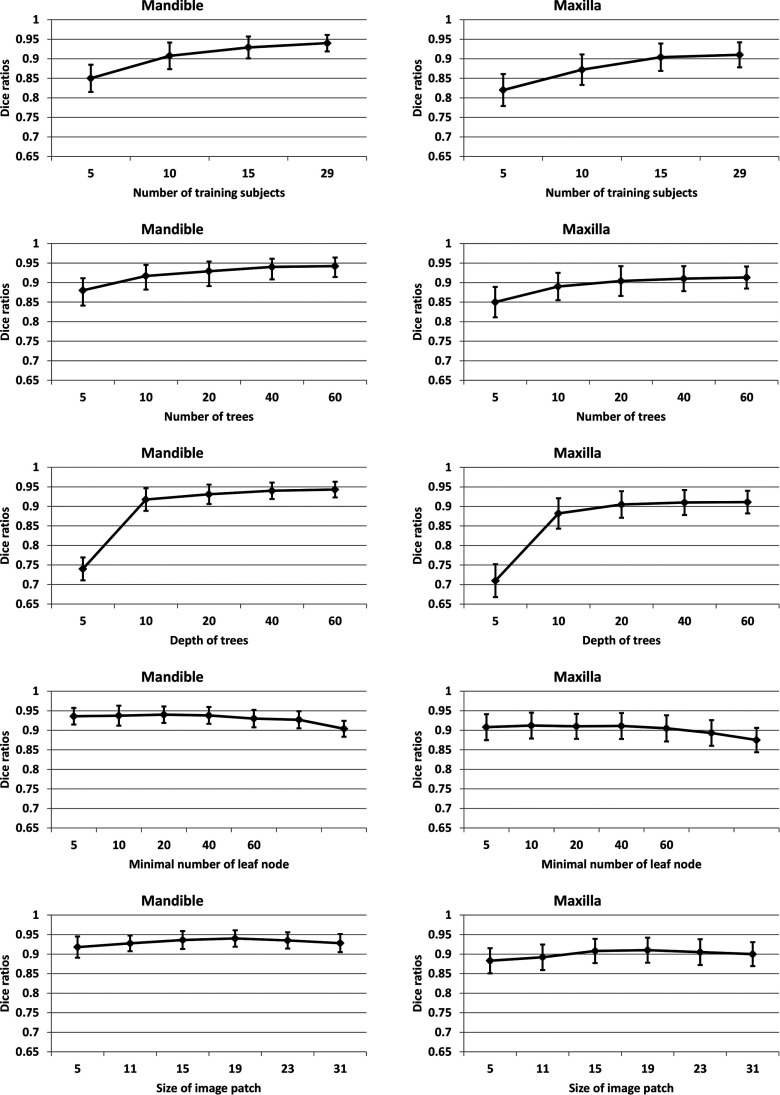
Number of training subjects. We first studied the impact of the number of training subjects on segmentation accuracy. Results are shown in the first row of Fig. 4. We conservatively set the number of tree to 50 and the maximal tree depth as 100. We further set the minimal number of samples for leaf node as 8 according to previous work.²⁵ Thus, in most cases, the stopping criterion was based on the minimal number of samples in the leaf node. Generally, more number of training subjects would lead to more accurate segmentation results. As shown in the first row, increasing the number of training subjects improved the segmentation accuracy, as the average Dice ratio increased from 0.85 $\left(N=5\right)$ to 0.94 $\left(N=29\right)$ for mandible and from 0.82 $\left(N=5\right)$ to 0.91 $\left(N=29\right)$ for maxilla. It is worth noting that the increase of the training subjects does not increase our testing time, which is different from other multiatlas based methods.^15,16,20,45

FIG. 4.

Influence of 5 different parameters: the number of training subjects (first row), the number of trees (second row), the depth of each tree (third row), the minimally allowed number of samples per the leaf node (fourth row), and the size of image patch size (last row).

Number of trees. The second row of Fig. 4 shows the influence of the number of trees on the segmentation accuracy. Generally, more number of trees would lead to more accurate segmentation results, but the training would also take longer time. In addition, note that when the number reaches a certain level, the further improvement of performance becomes minimal. In this paper, we chose 40 trees in each iteration.

Tree depth. The third row of Fig. 4 shows the impact of the maximally allowed depth of trees. In general, a low depth would be likely to underfitting, while a deep depth would be likely to overfitting. In our case, we found that the performance was gradually improved from depth of 5 to depth of 40, while keeping steady when the depth was over 40.

Minimal sample number for leaf node. The fourth row of Fig. 4 shows the impact of the minimally allowed number for the leaf node. This parameter implicitly sets the depth of our trees. The performance was steady when the number was less than 20. However, when it was larger than 50, the performance started decreasing. This might be due to the case that the samples with different labels would possibly fall into the same leaf node if a larger allowance was set, which would result in a fuzzy classification.

Patch size. The last row shows the influence of the patch size. The optimal patch size is related to the complexity of the anatomical structure.^16,46 And, too small or too large patch size would result in suboptimal performance. Therefore, in this paper, we selected the patch size as 17 × 17 × 17.

3.B. Importance of prior and sequential random forests

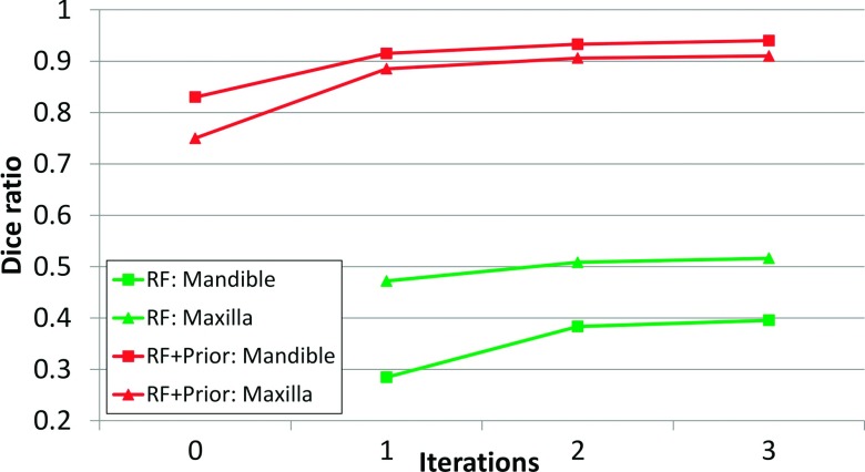
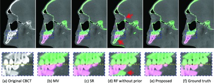
Figure 5 shows the Dice ratios on 30 CBCT images of CMF patients by applying a sequence of classifiers. The lower and upper two curves are the results by the sequential random forests without prior and with prior, respectively. At the beginning (#0 iteration), the Dice ratios were calculated upon the results by majority voting, which provided the prior for the sequential random forests. For the sequential random forests with prior, along the iterations, it could be seen that the Dice ratios were increasing and became stable after a few iterations. By contrast, for the sequential random forests without prior,²⁶ the results were much worse than the results with prior. The primary reason is due to the similar bony appearances shared by mandible, maxilla, and cervical vertebrae. Without the spatial prior, they could be mislabeled, as observed in Figs. 6(d) and 7(c). This comparison clearly demonstrates the importance of using (1) the prior in guiding the CBCT segmentation and (2) sequential random forests in further improving the accuracy.

FIG. 5.

The Dice ratios of mandible and maxilla on 30 CBCT subjects by the sequential random forests without prior lower two curves and with prior upper two curves.

FIG. 6.

Comparisons of segmentation results of different methods on (a) a typical CBCT image, (b) MV, (c) patch-based SR (Ref. 2), (d) stacked random forest without prior (Ref. 26), (e) the proposed stacked random forest with prior, and (f) ground truth.

FIG. 7.

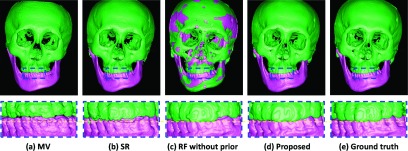
3D rendering surfaces obtained by different methods: (a) MV, (b) patch-based SR (Ref. 2), (c) sequential random forests without prior (Ref. 26), (d) the proposed sequential random forests with prior, and (e) ground truth.

3.C. Comparisons with the state-of-the-art methods

The validation was performed on 30 CBCT subjects in a leave-one-out strategy. In the following, we made qualitative and quantitative comparisons with the state-of-the-art methods. Figure 6 presents the segmentation results using different methods for one typical subject. From left to right, the first row shows the original CBCT image, and the results obtained by MV, patch-based SR,² sequential random forests without prior, the proposed sequential random forests with prior, and the manual segmentation. The second row shows the zoomed views for better visualization. Due to possible errors during affine registration, the result by MV was not accurate, which was however sufficient as a prior. For the SR, to achieve the best performance, we applied a nonlinear registration method (Elastix)⁴⁷ to align all atlases to the target subject. We also optimized the parameters for SR via cross validation. However, due to the closed-bite position and large intensity variations, SR (Ref. 2) still could not accurately separate the mandible from the maxilla. Without prior, the sequential random forests mislabel the maxilla and the mandible, as indicated by arrows. By contrast, the proposed prior-guided sequential random forests achieved a reasonable result, which was much consistent with the ground truth. The corresponding 3D surfaces generated by different methods are shown in Fig. 7, which also clearly demonstrates more consistency of our result with the ground truth than others. Moreover, the proposed prior-guided sequential random forests only required ∼20 min for segmentation of a typical set of CBCT images, where 5 min were used for MV and another 15 min were used for prior-guided sequential random forests in the testing stage (Table I). By contrast, the SR requires ∼5 h. Recall that it usually takes 12 h to manually segment a whole skull for every set of CBCT images. Therefore, our proposed method will be able to greatly improve the efficiency of CBCT segmentation for clinical applications. Of course, the speed of our algorithm can be significantly improved by code optimization and also GPU-based implementation.

TABLE I.

Average Dice ratios and surface-distance errors (in mm) on 30 CBCT subjects. The best performance is bolded. MV provides initial probabilities for our proposed method.

		MV	SR (Ref. 2)	RF without prior (Ref. 26)	Proposed (RF with prior)
Running time		5 m	5 h	15 m	20 m
Dice ratio	Mandible	0.83 ± 0.04	0.92 ± 0.03	0.51 ± 0.12	0.94 ± 0.02
	Maxilla	0.75 ± 0.04	0.88 ± 0.02	0.39 ± 0.14	0.91 ± 0.03
Average distance	Mandible	1.21 ± 0.25	0.62 ± 0.23	3.42 ± 1.21	0.42 ± 0.15
Hausdorff distance	Mandible	3.65 ± 1.53	0.95 ± 0.24	4.74 ± 2.56	0.74 ± 0.25

We then quantitatively evaluated the performance of different methods, with the results shown in Table I. Using prior and the sequential random forests, the proposed method achieved the highest Dice ratios. To further validate the proposed method, we also evaluated the accuracy by measuring the average surface-distance error (SDE), which is defined as

$${\displaystyle \text{SDE}\left(A,B\right)=\frac{1}{2}\left(\frac{1}{n_A}\sum _{a\in \text{surf}\left(A\right)}\text{dist}\left(a,B\right)+\frac{1}{n_B}\sum _{b\in \text{surf}\left(B\right)}\text{dist}\left(b,A\right)\right),}$$ (2)

where $\text{surf}\left(A\right)$ is the surface of segmentation A, n_A is the total number of surface points in $\text{surf}\left(A\right)$, and $\text{dist}\left(a,B\right)$ is the Euclidean distance between a surface point a and the nearest surface point of segmentation B. Additionally, the Hausdorff distance was also used to measure the maximal surface-distance errors of each of 30 subjects. The average surface distance and Hausdorff distance on all 30 CBCT subjects are shown in Table I, which again demonstrates the advantage of our proposed method.

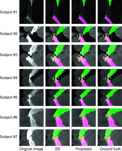
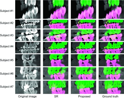
To further demonstrate the advantages of the proposed method in terms of separation of lower and upper teeth, Figs. 8 and 9 show the results by different methods on the teeth part (the incisors and canines and molars) from seven different subjects. The appearance varies from open-mouth to closed-bite in MI. Since the results by majority voting and sequential random forest without prior are much worse than our proposed results as indicated in Table I, in the following, we only focus on comparisons with SR.² As shown in Figs. 8 and 9, the proposed method can achieve more accurate results than SR,² especially for the close-bite cases. We also quantitatively measured the performance in the teeth part via Dice ratios, average surface distance, and Hausdorff distance. The measurements are shown in Table II, in which our method achieves significantly better results than SR (Ref. 2) (p-value < 0.001).

FIG. 8.

Comparisons of segmentation results on the incisors part from seven typical CBCTs.

FIG. 9.

Comparisons of segmentation results on the canines and molars part from seven typical CBCTs.

TABLE II.

Average Dice ratios and surface-distance errors (in mm) for the teeth part from 30 CBCTs.

		SR (Ref. 2)	Proposed
Dice ratio	Mandible	0.915 ± 0.024	0.958 ± 0.016
	Maxilla	0.893 ± 0.028	0.926 ± 0.021
Average distance	Mandible	0.723 ± 0.343	0.312 ± 0.103
	Maxilla	0.739 ± 0.411	0.346 ± 0.154
Hausdorff distance	Mandible	1.266 ± 0.316	0.618 ± 0.186
	Maxilla	1.361 ± 0.352	0.669 ± 0.209

3.D. Validation on MSCTs

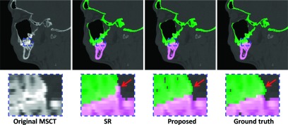
We also validated the proposed method on 60 spiral MSCT subjects scanned at maximal intercuspation. Their ages were 22 ± 2.6 yr (range: 18–27 yr). The MSCT images were acquired in a CT scanner (GE LightSpeed RT) with a matrix of 512 × 512, a resolution of 0.488 × 0.488 × 1.25 mm³, the time of exposure of less than 5 s, and a technique setting of 120 kVp and 120 mAs. Similar with the validation on CBCT images, we performed a twofold cross validation. The segmentation results by different methods on a typical MSCT are shown in Fig. 10. It can be seen from the zoomed views that the proposed method achieved a more accurate result than SR,² as indicated by arrows. We also quantitatively measured the performance as presented in Table III, which demonstrated the advantage of the proposed method.

FIG. 10.

Comparisons of segmentation results of different methods on a MSCT image.

TABLE III.

Average Dice ratios and surface-distance errors (in mm) on 60 MSCT subjects. The best performance is bolded.

		SR (Ref. 2)	Proposed (RF with prior)
Dice ratio	Mandible	0.93 ± 0.02	0.95 ± 0.02
	Maxilla	0.90 ± 0.02	0.92 ± 0.01
Average distance	Mandible	0.57 ± 0.22	0.33 ± 0.11
Hausdorff distance	Mandible	0.79 ± 0.19	0.41 ± 0.20

4. DISCUSSIONS

In our current work, considering the computational time and robustness, we employ just majority voting to estimate the initial prior for our prior-guided sequential random forests. Although it may be more reasonable to use the results by SR (Ref. 2) as prior due to their higher accuracy than majority voting, the computation of SR is expensive. Also, even with the low accuracy of majority voting, the proposed sequential random forests can still achieve better performance than the SR.

Although our proposed method can produce accurate results on CBCT images, it also has certain limitations. (1) The robustness of the proposed method may be further improved with more training subjects. Currently, our training subjects consist of only 30 CBCT scans, which may not be enough. In addition, only four subjects have streak artifacts caused by metallic implants. Consequently, the learned classifiers may still be somehow sensitive to the metal artifacts. (2) It takes around 20 min for our current pipeline to process a new set of CBCT scan. It needs to improve for the use in clinical applications. (3) In feature extraction, we extract the same feature type, i.e., 3D Haar-like features, from both the original CBCT images and probability maps, which may be not optimal. In our future work, we will employ more CBCT scans to train classifiers, improve the efficiency, and explore more feature types.

5. CONCLUSIONS

We have developed and validated a novel fully automated method for CBCT segmentation. We first estimate initial probability maps for mandible and maxilla, to provide a prior for the subsequent classifier training. We then extract both appearance features from CBCT and the context features from the initial probability maps to train the first-layer classifier via random forest. The first-layer classifier returns new probability maps. To deal with challenges of image artifacts and maximal intercuspation, the updated probability maps, together with the original CBCT features, are iteratively used to guide the training of the next classifier in the next round of training. Finally, a sequence of classifiers is learned. We have validated our proposed method on 30 CBCT subjects and additional 60 MSCT subjects with promising results.

REFERENCES

- 1.Xia J. J., Gateno J., and Teichgraeber J. F., “New clinical protocol to evaluate craniomaxillofacial deformity and plan surgical correction,” J. Oral Maxillofac. Surg. 67, 2093–2106 (2009). 10.1016/j.joms.2009.04.057 [DOI] [PMC free article] [PubMed] [Google Scholar]
- 2.Wang L., Chen K. C., Gao Y., Shi F., Liao S., Li G., Shen S. G. F., Yan J., Lee P. K. M., Chow B., Liu N. X., Xia J. J., and Shen D., “Automated bone segmentation from dental CBCT images using patch-based sparse representation and convex optimization,” Med. Phys. 41, 043503 (14pp.) (2014). 10.1118/1.4868455 [DOI] [PMC free article] [PubMed] [Google Scholar]
- 3.Le B. H., Deng Z., Xia J., Chang Y.-B., and Zhou X., “An interactive geometric technique for upper and lower teeth segmentation,” in Medical Image Computing and Computer-Assisted Intervention–MICCAI 2009, edited byYang G.-Z., Hawkes D., Rueckert D., Noble A., and Taylor C. (Springer Berlin Heidelberg, Berlin, 2009), Vol.5762, pp. 968–975. 10.1007/978-3-642-04271-3_117 [DOI] [PubMed] [Google Scholar]
- 4.Battan A. T., Beaudreau C. A., Weimer K. A., and Christensen A. M., in Effectiveness of Postprocessing Cone-Beam Computed Tomography Data, edited by Xia J. (Personal Communication with Engineers at Medical Modeling Inc., Houston, TX, 2013). [Google Scholar]
- 5.Hassan B. A., “Applications of cone beam computed tomography in orthodontics and endodontics,” Ph.D. thesis, Reading University, VU University Amsterdam, 2010. [Google Scholar]
- 6.He L., Zheng S. F., and Wang L., “Integrating local distribution information with level set for boundary extraction,” J. Visual Commun. Image Representation 21, 343–354 (2010). 10.1016/j.jvcir.2010.02.009 [DOI] [Google Scholar]
- 7.Kainmueller D., Lamecker H., Seim H., Zinser M., and Zachow S., “Automatic extraction of mandibular nerve and bone from cone-beam CT data,” in Medical Image Computing and Computer-Assisted Intervention–MICCAI 2009, edited byYang G.-Z., Hawkes D., Rueckert D., Noble A., and Taylor C. (Springer Berlin Heidelberg, Berlin, 2009), Vol. 5762, pp. 76–83. 10.1007/978-3-642-04271-3_10 [DOI] [PubMed] [Google Scholar]
- 8.Gollmer S. T. and Buzug T. M., “Fully automatic shape constrained mandible segmentation from cone-beam CT data,” in 9th IEEE International Symposium on Biomedical Imaging (ISBI) (IEEE, Barcelona, 2012), pp. 1272–1275. 10.1109/ISBI.2012.6235794 [DOI] [Google Scholar]
- 9.Zhang S., Zhan Y., Dewan M., Huang J., Metaxas D. N., and Zhou X. S., “Deformable segmentation via sparse shape representation,” in Medical Image Computing and Computer-Assisted Intervention–MICCAI 2011, edited byFichtinger G., Martel A., and Peters T. (Springer Berlin Heidelberg, Berlin, 2011), Vol. 6892, pp. 451–458. 10.1007/978-3-642-23629-7_55 [DOI] [PubMed] [Google Scholar]
- 10.Duy N., Lamecker H., Kainmueller D., and Zachow S., “Automatic detection and classification of teeth in CT data,” in Medical Image Computing and Computer-Assisted Intervention–MICCAI 2012, edited byAyache N., Delingette H., Golland P., and Mori K. (Springer Berlin Heidelberg, Berlin, 2012), Vol. 7510, pp. 609–616. 10.1007/978-3-642-33415-3_75 [DOI] [PubMed] [Google Scholar]
- 11.Zhang S., Zhan Y., Dewan M., Huang J., Metaxas D. N., and Zhou X. S., “Towards robust and effective shape modeling: Sparse shape composition,” Med. Image Anal. 16, 265–277 (2012). 10.1016/j.media.2011.08.004 [DOI] [PubMed] [Google Scholar]
- 12.Zhang S. T., Zhan Y. Q., and Metaxas D. N., “Deformable segmentation via sparse representation and dictionary learning,” Med. Image Anal. 16, 1385–1396 (2012). 10.1016/j.media.2012.07.007 [DOI] [PubMed] [Google Scholar]
- 13.Sabuncu M. R., Yeo B. T. T., Van Leemput K., Fischl B., and Golland P., “A generative model for image segmentation based on label fusion,” IEEE Trans. Med. Imaging 29, 1714–1729 (2010). 10.1109/TMI.2010.2050897 [DOI] [PMC free article] [PubMed] [Google Scholar]
- 14.Wang H., Suh J. W., Das S. R., Pluta J., Craige C., and Yushkevich P. A., “Multi-atlas segmentation with joint label fusion,” IEEE Trans. Pattern Anal. Machine Intell. 35, 611–623 (2013). 10.1109/tpami.2012.143 [DOI] [PMC free article] [PubMed] [Google Scholar]
- 15.Rousseau F., Habas P. A., and Studholme C., “A supervised patch-based approach for human brain labeling,” IEEE Trans. Med. Imaging 30, 1852–1862 (2011). 10.1109/TMI.2011.2156806 [DOI] [PMC free article] [PubMed] [Google Scholar]
- 16.Coupé P., Manjón J., Fonov V., Pruessner J., Robles M., and Collins D. L., “Patch-based segmentation using expert priors: Application to hippocampus and ventricle segmentation,” NeuroImage 54, 940–954 (2011). 10.1016/j.neuroimage.2010.09.018 [DOI] [PubMed] [Google Scholar]
- 17.Ta V.-T., Giraud R., Collins D. L., and Coupé P., “Optimized PatchMatch for near real time and accurate label fusion,” in Medical Image Computing and Computer-Assisted Intervention–MICCAI 2014, edited byGolland P., Hata N., Barillot C., Hornegger J., and Howe R. (Springer International Publishing, Berlin, 2014), Vol. 8675, pp. 105–112. 10.1007/978-3-319-10443-0_14 [DOI] [PubMed] [Google Scholar]
- 18.Aljabar P., Heckemann R. A., Hammers A., Hajnal J. V., and Rueckert D., “Multi-atlas based segmentation of brain images: Atlas selection and its effect on accuracy,” NeuroImage 46, 726–738 (2009). 10.1016/j.neuroimage.2009.02.018 [DOI] [PubMed] [Google Scholar]
- 19.Wang L., Shi F., Li G., Gao Y., Lin W., Gilmore J. H., and Shen D., “Segmentation of neonatal brain MR images using patch-driven level sets,” NeuroImage 84, 141–158 (2014). 10.1016/j.neuroimage.2013.08.008 [DOI] [PMC free article] [PubMed] [Google Scholar]
- 20.Wang L., Shi F., Gao Y., Li G., Gilmore J. H., Lin W., and Shen D., “Integration of sparse multi-modality representation and anatomical constraint for isointense infant brain MR image segmentation,” NeuroImage 89, 152–164 (2014). 10.1016/j.neuroimage.2013.11.040 [DOI] [PMC free article] [PubMed] [Google Scholar]
- 21.Shi F., Wang L., Wu G. R., Li G., Gilmore J. H., Lin W. L., and Shen D., “Neonatal atlas construction using sparse representation,” Hum. Brain Mapp. 35, 4663–4677 (2014). 10.1002/hbm.22502 [DOI] [PMC free article] [PubMed] [Google Scholar]
- 22.Breiman L., “Random forests,” Mach. Learn. 45, 5–32 (2001). 10.1023/A:1010933404324 [DOI] [Google Scholar]
- 23.Zikic D., Glocker B., Konukoglu E., Criminisi A., Demiralp C., Shotton J., Thomas O. M., Das T., Jena R., and Price S. J., “Decision forests for tissue-specific segmentation of high-grade gliomas in multi-channel MR,” in Medical Image Computing and Computer-Assisted Intervention–MICCAI 2012, edited byAyache N., Delingette H., Golland P., and Mori K. (Springer Berlin Heidelberg, Berlin, 2012), Vol. 7512, pp. 369–376. 10.1007/978-3-642-33454-2_46 [DOI] [PubMed] [Google Scholar]
- 24.Zikic D., Glocker B., and Criminisi A., “Encoding atlases by randomized classification forests for efficient multi-atlas label propagation,” Med. Image Anal. 18, 1262–1273 (2014). 10.1016/j.media.2014.06.010 [DOI] [PubMed] [Google Scholar]
- 25.Zikic D., Glocker B., and Criminisi A., “Atlas encoding by randomized forests for efficient label propagation,” in Medical Image Computing and Computer-Assisted Intervention–MICCAI 2013 (Springer Berlin Heidelberg, Berlin, 2013), Vol. 8151, pp. 66–73. 10.1007/978-3-642-40760-4_9 [DOI] [PubMed] [Google Scholar]
- 26.Wang L., Gao Y., Shi F., Li G., Gilmore J. H., Lin W., and Shen D., “LINKS: Learning-based multi-source integration framework for segmentation of infant brain images,” NeuroImage 108, 160–172 (2015). 10.1016/j.neuroimage.2014.12.042 [DOI] [PMC free article] [PubMed] [Google Scholar]
- 27.Criminisi A., Shotton J., and Konukoglu E., “Decision forests: A unified framework for classification, regression, density estimation, manifold learning and semi-supervised learning,” Found. Trends® Comput. Graphics Vision 7, 81–227 (2012). 10.1561/0600000035 [DOI] [Google Scholar]
- 28.Glocker B., Pauly O., Konukoglu E., and Criminisi A., “Joint classification-regression forests for spatially structured multi-object segmentation,” Lect. Notes Comput. Sci. 7575, 870–881 (2012). 10.1007/978-3-642-33765-9_62 [DOI] [Google Scholar]
- 29.Tu Z. and Bai X., “Auto-context and its application to high-level vision tasks and 3D brain image segmentation,” IEEE Trans. Pattern Anal. Machine Intell. 32, 1744–1757 (2010). 10.1109/tpami.2009.186 [DOI] [PubMed] [Google Scholar]
- 30.Loog M. and Ginneken B., “Segmentation of the posterior ribs in chest radiographs using iterated contextual pixel classification,” IEEE Trans. Med. Imaging 25, 602–611 (2006). 10.1109/TMI.2006.872747 [DOI] [PubMed] [Google Scholar]
- 31.Viola P. and Jones M. J., “Robust real-time face detection,” Int. J. Comput. Vision 57, 137–154 (2004). 10.1023/B:VISI.0000013087.49260.fb [DOI] [Google Scholar]
- 32.Sutton C., McCallum A., and Rohanimanesh K., “Dynamic conditional random fields: Factorized probabilistic models for labeling and segmenting sequence data,” J. Mach. Learn. Res. 8, 693–723 (2007), see https://people.cs.umass.edu/~mccallum/papers/dcrf-jmlr2007.pdf. [Google Scholar]
- 33.Oliva A. and Torralba A., “The role of context in object recognition,” Trends Cognit. Sci. 11, 520–527 (2007). 10.1016/j.tics.2007.09.009 [DOI] [PubMed] [Google Scholar]
- 34.Belongie S., Malik J., and Puzicha J., “Shape matching and object recognition using shape contexts,” IEEE Trans. Pattern Anal. Machine Intell. 24, 509–522 (2002). 10.1109/34.993558 [DOI] [PubMed] [Google Scholar]
- 35.Geman S. and Geman D., “Stochastic relaxation, Gibbs distributions, and the Bayesian restoration of images,” IEEE Trans. Pattern Anal. Machine Intell. 6, 721–741 (1984). 10.1109/tpami.1984.4767596 [DOI] [PubMed] [Google Scholar]
- 36.Hsu C.-W. and Lin C.-J., “A comparison of methods for multiclass support vector machines,” IEEE Trans. Neural Networks 13, 415–425 (2002). 10.1109/72.991427 [DOI] [PubMed] [Google Scholar]
- 37.Criminisi A., Shotton J., and Bucciarelli S., “Decision forests with long-range spatial context for organ localization in CT volumes,” in MICCAI Workshop on Probabilistic Models for Medical Image Analysis (MICCAI-PMMIA) (2009). [Google Scholar]
- 38.Lowe D. G., “Object recognition from local scale-invariant features,” in Proceedings of the Seventh IEEE International Conference on Computer Vision (IEEE, Kerkyra, 1999), Vol. 1152, pp. 1150–1157. 10.1109/ICCV.1999.790410 [DOI] [Google Scholar]
- 39.Dalal N. and Triggs B., in Presented at the IEEE Computer Society Conference on Computer Vision and Pattern Recognition (CVPR) (2005). [Google Scholar]
- 40.Ahonen T., Hadid A., and Pietikainen M., “Face description with local binary patterns: Application to face recognition,” IEEE Trans. Pattern Anal. Machine Intell. 28, 2037–2041 (2006). 10.1109/TPAMI.2006.244 [DOI] [PubMed] [Google Scholar]
- 41.Han X., “Learning-boosted label fusion for multi-atlas auto-segmentation,” in Machine Learning in Medical Imaging, edited byWu G., Zhang D., Shen D., Yan P., Suzuki K., and Wang F. (Springer International Publishing, Berlin, 2013), Vol. 8184, pp. 17–24. 10.1007/978-3-319-02267-3_3 [DOI] [Google Scholar]
- 42.Cheng H., Liu Z., and Yang L., in Presented at the IEEE 12th International Conference on Computer Vision (2009). [Google Scholar]
- 43.Wright J., Yi M., Mairal J., Sapiro G., Huang T. S., and Shuicheng Y., “Sparse representation for computer vision and Pattern recognition,” Proc. IEEE 98, 1031–1044 (2010). 10.1109/JPROC.2010.2044470 [DOI] [Google Scholar]
- 44.Bach F., Mairal J., and Ponce J., “Task-driven dictionary learning,” IEEE Trans. Pattern Anal. Machine Intell. 34, 791–804 (2012). 10.1109/tpami.2011.156 [DOI] [PubMed] [Google Scholar]
- 45.Srhoj-Egekher V., Benders M. J. N. L., Viergever M. A., and Išgum I., “Automatic neonatal brain tissue segmentation with MRI,” Proc. SPIE 8669, 86691K (2013). 10.1117/12.2006653 [DOI] [Google Scholar]
- 46.Tong T., Wolz R., Coupé P., Hajnal J. V., and Rueckert D., “Segmentation of MR images via discriminative dictionary learning and sparse coding: Application to hippocampus labeling,” NeuroImage 76, 11–23 (2013). 10.1016/j.neuroimage.2013.02.069 [DOI] [PubMed] [Google Scholar]
- 47.Klein S., Staring M., Murphy K., Viergever M. A., and Pluim J., “Elastix: A toolbox for intensity-based medical image registration,” IEEE Trans. Med. Imaging 29, 196–205 (2010). 10.1109/TMI.2009.2035616 [DOI] [PubMed] [Google Scholar]