Missing data exploration: highlighting graphical presentation of missing pattern

Abstract

Functions shipped with R base can fulfill many tasks of missing data handling. However, because the data volume of electronic medical record (EMR) system is always very large, more sophisticated methods may be helpful in data management. The article focuses on missing data handling by using advanced techniques. There are three types of missing data, that is, missing completely at random (MCAR), missing at random (MAR) and not missing at random (NMAR). This classification system depends on how missing values are generated. Two packages, Multivariate Imputation by Chained Equations (MICE) and Visualization and Imputation of Missing Values (VIM), provide sophisticated functions to explore missing data pattern. In particular, the VIM package is especially helpful in visual inspection of missing data. Finally, correlation analysis provides information on the dependence of missing data on other variables. Such information is useful in subsequent imputations.

Zhongheng Zhang, MMed.

Introduction

The previous article of big-data clinical trial series has introduced basic techniques in dealing with missing values. There are several R packages that allow advanced methods for managing missing data. Some useful methods include visual presentation of missing data pattern and correlation analysis (1). This article firstly creates a dataset containing five variables. Three missing data classes are illustrated in creating the dataset by simulation. Then various tools for the exploration of missing data are introduced.

Classification of missing data

Statisticians typically classify missing data into three categories. Missing completely at random (MCAR) refers to the presence of missing values on a variable that is unrelated to any other observed and unobserved variables (2,3). In other words, there is no systematic reason for the missing pattern. Missing at random (MAR) is the presence of missing values on a variable that is related to other observed variables but not related to its own unobserved values. Not missing at random (NMAR) is the presence of missing values on a variable that is neither MCAR nor MAR. For example, a patient with lower lactate value is more likely to have a missing lactate value. A hemodynamically stable patient typically has a lower lactate value. In the situation, a treating physician is less likely to order test for lactate.

Dataset simulation

A dataset of 200 observations is created by simulation. The dataset is used for illustration purpose and there is no clinical relevance. There are five variables including age, sex, lactate (lac), white blood cell (wbc) and C-reactive protein (crp). In each simulation, I set a seed to allow readers to replicate the results.

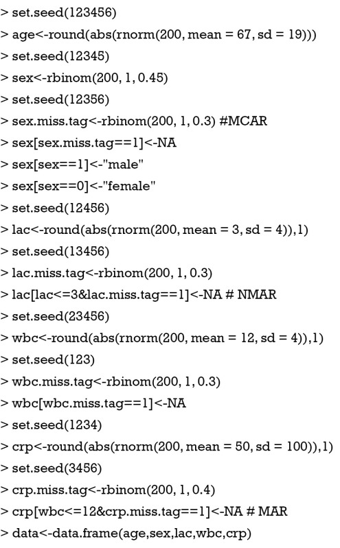
The variable age has complete values for all observations. It is assumed that our population has mean age of 67 with standard deviation of 19. The abs() function is employed to avoid negative values. The results are rounded to integers by using round() function with default argument for decimal place. The variable sex is a categorical variable and it is assumed to have binominal distribution. Missing values on sex is set to MCAR. The variable lac has normal distribution with a mean value of 3 and a standard deviation of 4. It is set to NMAR and missing values occur more likely at lac values equal to or less than 3. The variable wbc has a normal distribution and missing values are MCAR. The variable crp assumes a normal distribution and missing values occur more frequently at wbc values equal to or less than 12. The rationale behind this missing pattern is that in clinical practice physicians may first order white blood cell count and for those with high WBC values they will further order test for crp.

Exploring missing pattern with md.pattern() function

The md.pattern() function shipped with Multivariate Imputation by Chained Equations (MICE) package can be used to produce a table displaying the missing pattern (4).

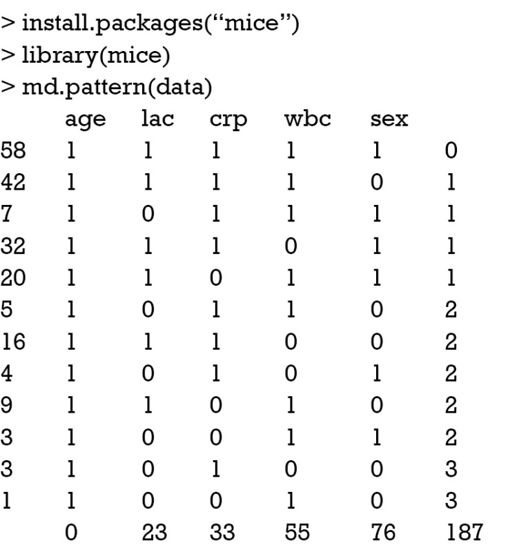
In the main body of the output table, “1” indicates nonmissing value and “0” indicates missing value. The first column shows the number of unique missing data patterns. There are 58 observations with nonmissing values, and there are 42 observations with nonmissing values except for the variable sex. The rightmost column shows the number of missing variables in a particular missing pattern. For example, the first row has no missing value and it is “0” in the row. The last row counts the number of missing values for each variable. For example, the variable age contains no missing values and the variable crp contains 33 missing values. This table can be helpful when you decide to drop some observations with missing variables exceeding a preset threshold.

Visual presentation of missing data pattern

Although the above table displays missing pattern compactly and effectively, you may also want to show it in a figure. As the saying goes “one look is worth a thousand words.” The Visualization and Imputation of Missing Values (VIM) package is very powerful in visually displaying missing data pattern (5). This package contains advanced tools for the visualization of missing or imputed values. It is helpful for exploring the structure of the missing or imputed values. The missing data pattern is essential for selecting an appropriate imputation method to estimate missing values. Thus the visualization tools should be applied before imputation and the diagnostic tools afterwards. There are three functions can be used for this purpose: matrixplot(), scattMiss() and aggr().

Click in a column to sort by the corresponding variable.

To regain use of the VIM GUI and the R console, click outside the plot region.

Matrix plot sorted by variable ‘wbc’.

The matrixplot() is interactive and when the message “Click in a column to sort by the corresponding variable” pops up, I click on the wbc column. The result is shown in Figure 1. In the figure, missing values are represented in red. The continuous variable is rescaled and represented by grayscale colors. Lighter colors indicate lower values and darker colors suggest larger values. Note that missing values on crp occur only at lower levels of wbc, which is consistent with the rule in running the simulation. Because I choose to sort by the wbc variable, it is displayed firstly with missing values and then in descending order.

Figure 1.

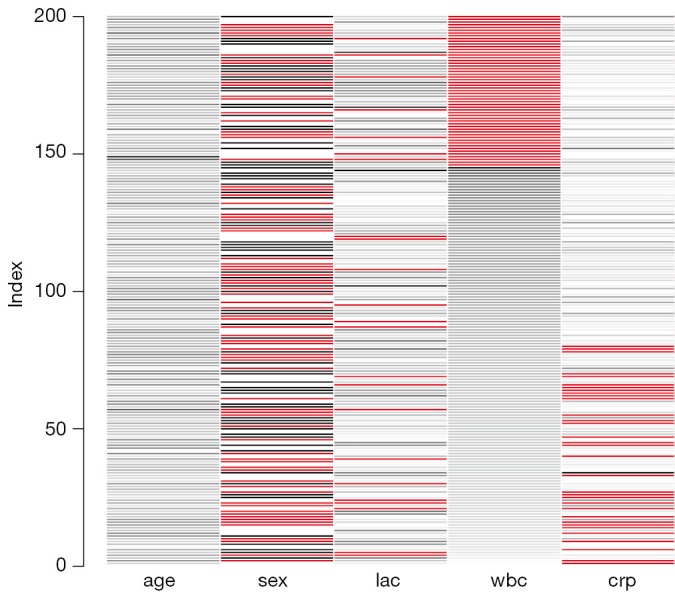
Matrix plot of nonmissing and missing values by observations. The matrix is sorted by the variable wbc.

Click in in the left margin to switch to the previous variable or in the right margin to switch to the next variable.

To regain use of the VIM GUI and the R console, click anywhere else in the graphics window.

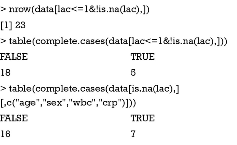
The barMiss() and histMiss() functions produce similar figures and I would like to illustrate barMiss() only. By default, barMiss() produce interactive plot and one can click to choose on which variable to display. Here, I displayed lac variable. The horizontal axis is lac values. Figure 2 displays barplot with highlighting of missing values in other variables by splitting each bar into two parts. Additionally, information about missing values in the variable lac is shown on the right hand side. There are 23 observations with lac ≤1. Of the 23 observations, there are 18 cases with missing values on other variables and 5 cases contain no missing values on other variables. The right hand side bar shows there are 23 missing values on the variable lac. Of them, there are 16 cases with missing values on other variables and 7 cases contain no missing values on other variables.

Figure 2.

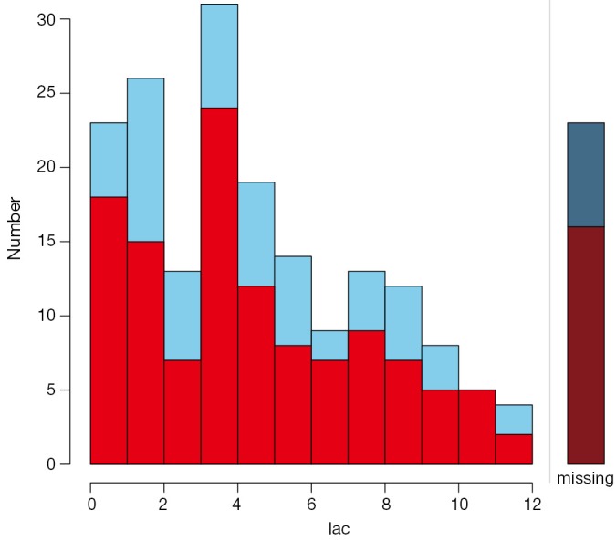
Barplot highlighting missing values in other variables by splitting each bar into two parts. One part represents missing values and the other represents nonmissing values.

The aggr() function produces missing data pattern as shown in Figure 3. The left panel displays proportion of missing values on each variable. As expected, age has no missing values and lac has around 10% missing values. The right panel expresses the same information as the table produced by md.pattern() function. There are 58 complete observations without missing values. 42 observations contain missing values only on sex.

Figure 3.

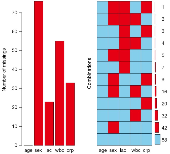
Missing data pattern produced by aggr() function.

The result of marginplot() is shown in Figure 4. Nonmissing values are displayed in green color and missing values are in red color. There are 33 missing values on crp, and the mean value of wbc with missing values on crp is around 9. Wbc with missing values on crp is significantly lower than wbc with complete values on crp (comparing horizontal red and green box plots). However, there is no difference between crp values in cases with and without missing values on wbc (vertical red and green box plots).

Figure 4.

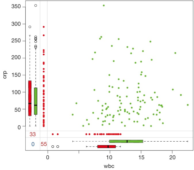
Scatter plot between wbc and crp, with missing values displayed on the margins.

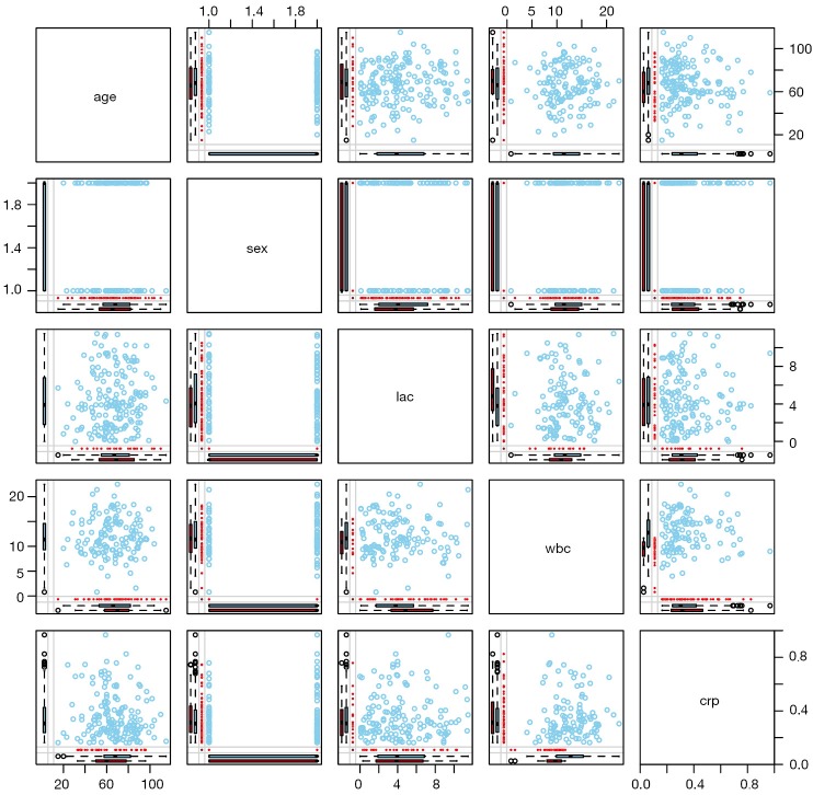
This is an extension of the marginplot() function that creates a scatterplot matrix with information about missing values in the plot margins of each panel (Figure 5). Interpretation of each panel is the same as Figure 4.

Figure 5.

Scatterplot matrix with information about missing values in the plot margins of each panel.

Click in the left margin to switch to the previous variable or in the right margin to switch to the next variable.

To regain use of the VIM GUI and the R console, click anywhere else in the graphics window.

The spineMiss() function produces plot similar to that produced by barMiss(). The spineplot highlights of missing values in other variables by splitting each cell into two parts (Figure 6). Additionally, information about missing values in the variable of interest (lac) is shown on the right hand side. The vertical axis is proportion instead of counts in barplot produced by barMiss() function.

Figure 6.

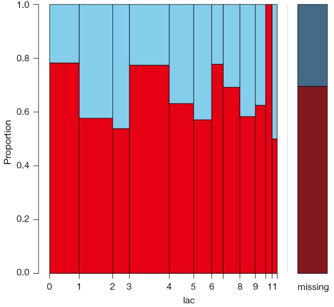
Spineplot highlighting missing values in other variables by splitting each cell into two parts. Additionally, information about missing values in the variable lac is shown on the right hand side.

Click in a diagonal panel to add to or remove from the highlight selection.

To regain use of the VIM GUI and the R console, click anywhere else in the graphics window.

Highlighted missing in any of the variables ‘age’, ‘sex’, ‘lac’, ‘wbc’, ‘crp’.

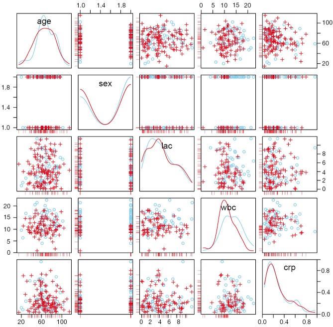
The scattmatrixMiss() produces Scatterplot matrix in which cases with missing values in certain variables (‘age’, ‘sex’, ‘lac’, ‘wbc’, ‘crp’) are highlighted (Figure 7). Variables with missing values to be highlighted can be added or removed by clicking in a diagonal panel. The diagonal panels display density plots for non-highlighted and highlighted observations. The red-cross symbols represent observations with missing values on any of the variables age, sex, lac, wbc and crp.

Figure 7.

Scatterplot matrix in which observations with missing values in certain variables (age, sex, lac, wbc, crp) are highlighted.

Exploring missing data pattern by correlation matrix

Correlation matrix can be utilized to explore which two variables tend to have missing values together, or the relationship between the presence of missing values in a variable and the observed values on other variables. To complete this task, one may need to create a shadow matrix in which missing values are replaced by “1”, and nonmissing values are replaced by “0”.

Next, you can create a new data frame in which only variables with one or more missing values are retained.

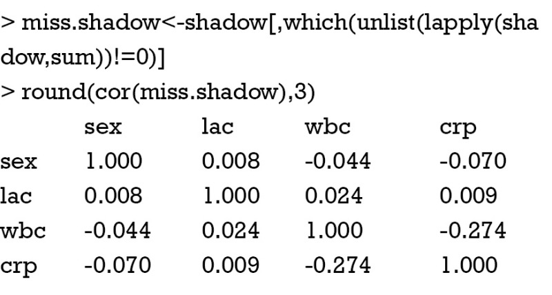
There is no strong correlation among these variables and one can safely conclude that the presence of missing values in one variable is not related to missing values in other variables. Next, you can examine the relationship between the presence of missing values in a variable and the observed values on other variables. Before running the cor() function, you need to retain only numeric variable in the first argument of cor() function. The round() function is again used to make the output more succinct.

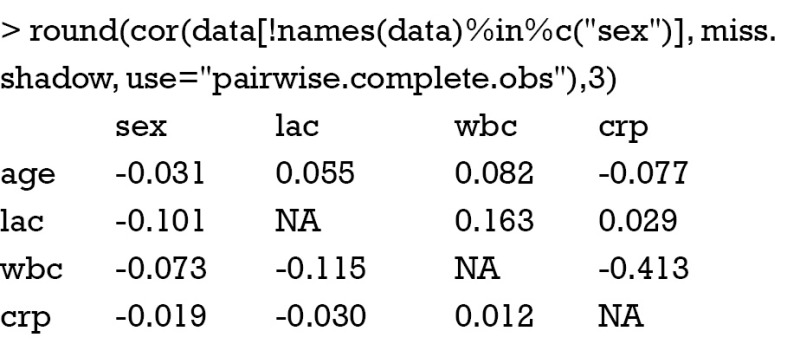
As you can see there is a negative correlation between crp and wbc (r=-0.413), indicating that missing values on crp are more likely to occur at lower levels of wbc. The command is a little complex. The “names(data)%in%c(“sex”)” returns a logical vector with TRUE for each element in names(data) that matches “sex” and FALSE otherwise. The “!” symbol reverses the values of the logical vector. However, correlation analysis cannot replace using external information to judge whether missing data are NMAR. In other words, judgment from subject-matter knowledge is of critical importance to rule out NMAR.

Summary

Missing data is ubiquitous in big-data clinical research and sometimes the mechanisms underlying the missing pattern may be complicated. In this situation some advanced techniques in dealing with missing data may be helpful. Classified by the mechanism of missing, there are three types of missing data including MCAR, MAR and NMAR. While imputations depending on other covariates can be used for the first two types, subject-matter knowledge is required in dealing with the last type. Missing patterns can be illustrated in table manner. Furthermore, the VIM package provided many functions for graphical presentation of missing data. Relationships between missing data and values of other variables provide further insights into mechanisms underlying missing data. This can be explored by using correlation analysis.

Biography

Author’s introduction: Zhongheng Zhang, MMed. Department of Critical Care Medicine, Jinhua Municipal Central Hospital, Jinhua Hospital of Zhejiang University. Dr. Zhongheng Zhang is a fellow physician of the Jinhua Municipal Central Hospital. He graduated from School of Medicine, Zhejiang University in 2009, receiving Master Degree. He has published more than 35 academic papers (science citation indexed) that have been cited for over 200 times. He has been appointed as reviewer for 10 journals, including Journal of Cardiovascular Medicine, Hemodialysis International, Journal of Translational Medicine, Critical Care, International Journal of Clinical Practice, Journal of Critical Care. His major research interests include hemodynamic monitoring in sepsis and septic shock, delirium, and outcome study for critically ill patients. He is experienced in data management and statistical analysis by using R and STATA, big data exploration, systematic review and meta-analysis.

References

- 1.Kabacoff R. R in Action. Shelter Island: Manning Publications Co., 2011. [Google Scholar]
- 2.Montez-Rath ME, Winkelmayer WC, Desai M. Addressing missing data in clinical studies of kidney diseases. Clin J Am Soc Nephrol 2014;9:1328-35. [DOI] [PMC free article] [PubMed] [Google Scholar]
- 3.Dziura JD, Post LA, Zhao Q, et al. Strategies for dealing with missing data in clinical trials: from design to analysis. Yale J Biol Med 2013;86:343-58. [PMC free article] [PubMed] [Google Scholar]
- 4.Buuren SV, Groothuis-Oudshoorn K. mice: Multivariate Imputation by Chained Equations in R. Journal of Statistical Software 2011;45:1-67. [Google Scholar]
- 5.Templ M, Alfons A, Kowarik A, et al. Package VIM: Visualization and Imputation of Missing Values (2013). R package version 3.0. 3.1.