The Dynamic Process of Drug-GPCR Binding at Either Orthosteric or Allosteric Sites Evaluated by Metadynamics

Abstract

Major advances in G Protein-Coupled Receptor (GPCR) structural biology over the past few years have yielded a significant number of high-resolution crystal structures for several different receptor subtypes. This dramatic increase in GPCR structural information has underscored the use of automated docking algorithms for the discovery of novel ligands that can eventually be developed into improved therapeutics. However, these algorithms are often unable to discriminate between different, yet energetically similar, poses because of their relatively simple scoring functions. Here, we describe a metadynamics-based approach to study the dynamic process of ligand binding to/unbinding from GPCRs with a higher level of accuracy and yet satisfying efficiency.

1 Introduction

Several technological breakthroughs (e.g., lipid cubic phase and receptor constructs stabilized by specific amino acid mutations or proteins [1]) have enabled the successful determination of several high-resolution crystal structures of G Protein-Coupled Receptors (GPCRs) over the past few years [2, 3]. Although the majority of these structures have been solved in an inactive conformation with inverse agonists bound at the orthosteric site (i.e., the binding site recognized by endogenous agonists), a few GPCR structures have also revealed the location of allosteric sites (e.g., see [4]) or features that have been attributed to active GPCR conformations (e.g., see [5]).

Notwithstanding the continuously growing number of high-resolution structures of GPCRs, it is anticipated that not all ligand–GPCR complexes can or will be crystallized in the near future. Thus, computational methods that can accurately predict GPCR binding sites and stable ligand poses offer a unique opportunity to fill a possible information gap in structural biology, and create a solid basis for discovering novel compounds. Although several automated docking algorithms have been successfully applied to predict the binding site of various GPCRs of known structure [6], the semiempirical scoring functions used to yield rough estimates of binding affinity for high-throughput performance are often unable to discriminate between differently stable ligand poses [7, 8].

More sophisticated techniques such as all-atom molecular dynamics (MD) simulations have proven to be a viable, albeit more computationally expensive, alternative to study ligand binding to a GPCR. There have been several advances over the past few years in both software implementation (e.g., Desmond [9], Gromacs [10], NAMD [11], and Blue Matter [12]) and computer hardware (e.g., Anton [13] or BlueGene [14, 15]) that have significantly impacted the MD field. Among them, specialized computer architectures such as Anton from the D.E. Shaw Research group have allowed to observe, within microsecond timescales, ligand binding from the bulk solvent to either orthosteric [16, 17] or allosteric sites [18] of GPCRs embedded into physiologically relevant lipid–water environments. However, ligand dissociation from the receptor did not occur within the simulated timescale of standard MD, thus preventing quantification of dissociation rate constants from these unbiased MD simulations of GPCRs. Another limitation of these approaches is that they require several million core hours on fairly expensive special-purpose computer resources, which are currently accessible only to a restricted group of investigators.

To overcome these important limitations, we designed a computational strategy that works within the framework of classical all-atom MD simulations, and uses an enhanced sampling algorithm called metadynamics [19] to efficiently study ligand binding to and unbinding from a GPCR. According to its original formulation by the Parrinello group, metadynamics allows to accelerate the sampling of specific degrees of freedom of the system by adding a history-dependent term acting on a small number of collective variables (CVs) to the standard force-field potential. The CVs are chosen to describe putatively relevant degrees of freedom of the system under study. This technique has been reported to be useful in predicting bound states for several biological systems in which the ligand had been initially placed in the bulk solvent [20–23]. We pioneered its use to predict ligand binding to GPCRs through an application to opioid receptors (ORs) [24], when a crystal structure for these receptors was not available yet. Since the original formulation of metadynamics did not allow to efficiently explore the states of the ligand in the bulk solvent, we combined it with a strategy originally put forward by the Roux lab [25, 26] to overcome this limitation. By restraining sampling of the ligand in the bulk, this strategy allowed to estimate the free-energy difference between an unbound reference state and a putative initial contact between the ligand and the receptor. This value was then used in combination with free-energy estimates of bound states sampled by metadynamics to calculate the overall binding free-energy. The latter allowed us to predict binding affinities for δ-OR ligands in line with experimental values [24].

Here, we present the metadynamics-based protocol we developed to accelerate the rate at which MD can sample relevant conformations of ligand–GPCR complexes, and provide quantitative estimates of ligand binding affinities.

2 Materials

The protocol described in this chapter has been implemented and tested using the software packages and Web-based tools listed below. It must be noted, however, that several different options enable the type of simulations discussed in the following sections and can be used based on personal preference and availability. Most of the codes used for these simulations are accessible to academic researches free of charge, although open-source alternatives to the employed commercial packages are also available (see ^{Note 1}).

1. Missing loops are modeled using Rosetta [27] or Modeller [28].

2. Parameterization of the ligand force-field is obtained using the Paramchem webserver [29–31], and the resulting parameters are validated and optimized using Gaussian [32] or Jaguar [33].

3. A model membrane (e.g., a 1-palmitoyl-2-oleoyl-phosphatidyl choline (POPC)-cholesterol bilayer) is generated using the CHARMM-gui webserver [34–36], and the receptor is embedded into the resulting lipid patch using the inflategro perl script [37]. We mention in passing that a revised and improved version of this script was recently made available by its developers [38].

4. MD equilibrations and production metadynamics simulations of the hydrated system are run using Gromacs 4.6.5 [39] and Plumed 1.3 [40]. The same simulations can be easily implemented with the newest versions Gromacs 5 and Plumed 2.

5. Post-processing and analysis of the simulations are performed using Gromacs and Plumed tools. The results are visualized using VMD [41], Pymol [42], and R scripts.

3 Methods

Please refer to Fig. 1 for a flow diagram of our proposed computational protocol to study drug–GPCR binding.

Fig. 1.

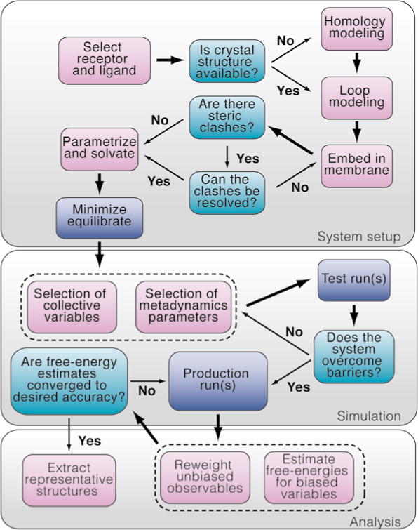
Flow diagram of the proposed computational protocol to study drug–GPCR binding

3.1 System Setup

1. Fetch a GPCR crystal structure (if available): The main source for experimentally solved GPCR structures is the pdb.org website where crystallographic structures are deposited and made publicly available. Focused databases on GPCR crystal structures also exist and are readily accessible (e.g., see GPCR-EXP maintained by the Yang Zhang lab [43]). Figure 2 shows a two-dimensional embedding of the root mean square differences among the currently listed GPCR structures in GPCR-EXP. When more than one experimentally derived conformational state is available, the appropriate active or inactive receptor conformation for simulation is selected depending on whether the ligand of interest is an agonist or an inverse agonist/antagonist. Please see ^{Note 2} for cases in which no crystal structures are available for the GPCR of interest.

2. Build missing extracellular (EC) loop segments: Due to their high flexibility, loop regions may not be resolved, or may be missing pieces, even in the context of high-resolution crystal structures. Since EC loop regions are known to play a role in the GPCR binding process, missing segments must be reconstructed. We have used homology modeling and/or protein threading (e.g., with Modeller [44]) to build missing loop segments only if crystal structures of highly homologous GPCRs were available for use as structural templates. In the absence of suitable crystal structures, we have given preference to ab-initio methods such as the one implemented in Rosetta [45] for the construction of loop regions. In contrast, we have often chosen to ignore the usually long and disordered N-terminal tail of receptors despite its potentially significant role in ligand binding (see ^{Note 3}).

3. Embed the receptor into a lipid bilayer: Several different approaches exist to generate a receptor–membrane system that is suitable for MD simulations. We usually use the CHARMM-gui webserver [36] to generate an initial membrane patch that is sufficiently large to accommodate the ligand–receptor complex under investigation. Typically, the side of the membrane patch is set to be at least 75 Å, which corresponds to roughly 170 lipid and sterol molecules. For the simulations described herein, we have used a 90:10 % mixture of POPC and cholesterol lipids. After the membrane is created, the inflategro script [37] is used to embed the receptor into the membrane. The inflategro script inflates the membrane around the receptor and reconstructs it in a stepwise process consisting of deflation and equilibration steps that can be stopped as soon as the membrane reaches the correct area per lipid value (in the case of the aforementioned POPC/10 % cholesterol patch, A = 61 Ų). The resulting structure is then analyzed for possible steric clashes of the lipids with the receptor side chains. Although small steric clashes are likely to resolve themselves during equilibration, other structural inconsistencies may require rerunning the deflation procedure and/or stopping the deflation at an earlier stage.

4. Placement of the ligand: The ligand may either be added to a non-equilibrated simulation box in a docked pose (e.g., using docking software such as AUTODOCK [46] or DOCK [47], etc.) or at a random position above the receptor (e.g., obtained manually with Pymol). As the results of metadynamics simulations do not depend on the initial conformation, it is irrelevant how the ligand is added to the simulation box. However, higher sampling efficiency may be achieved by starting from different positions of the ligand and employing the multiple-walker variant of metadynamics (see Subheading 3.5).

5. System hydration: The system is hydrated with the genbox tool in the Gromacs package, using a water model that is appropriate for the force field being used. We typically use the CHARMM force field, and hydrate the system with the TIP3P water model. Following hydration, the system is carefully checked for water molecules that might have been placed in the membrane. To limit the amount of misplaced water molecules, one can slightly increase (roughly by no more than 0.05 nm) the van der Waals radii of the carbon atoms listed in the vdwradii.dat file in the Gromacs topology folder. The changes in the vdwradii.dat will only influence the placement of the solvent using genbox and will not be taken into account during the simulation. Finally, ions are added to neutralize the system and, if desired, to reach physiological salt concentration. Typical systems prepared following these guidelines are 75 Å × 75 Å × 100 Å in size and contain ~70,000 atoms.

Fig. 2.

Two-dimensional embedding of the root mean square differences among the available GPCRs structures (Zhang’s Lab list as of October 2014). PDB labels of the various different crystal structures of inactive rhodopsin and adrenergic receptors were removed for the sake of clarity

3.2 Force Field and Ligand Parameterization

1. Choice of the force field: While several different force fields allow a reasonably accurate description of proteins and lipids, parameters for small-molecule ligands are often less precise and need re-parameterization (see below). We normally use the CHARMM force field [48] to describe GPCRs embedded into a lipid–water environment, and recommend to download CHARMM36 files [49] from the MacKerell lab website [50] until further developments become available.

2. Ligand parameterization: We use the Paramchem webserver to conveniently generate CHARMM General Force Field (CGenFF) parameters of the ligand. Briefly, these parameters are obtained by matching fragments of the ligand under study with molecules that have been carefully parameterized to be fully compatible with the CHARMM force field. The accuracy of this match is reported along with the parameters, and its value used to decide whether or not ab initio re-parameterization is needed (see ^{Note 4}). Should the CGenFF parameters be acceptable, the cgenff_charmm2gmx python script is used to convert them into the Gromacs format prior to their inclusion in the topology file.

3.3 System Equilibration

1. Minimization: Steepest descent minimization of the GPCR system embedded into a lipid bilayer is carried out for approximately 50,000 steps.

2. Equilibration: To first equilibrate the solvent around the macromolecules, a short (1 ns) dynamics run in the constant number of particles, volume, and temperature (NVT) ensemble is conducted by restraining the positions of the heavy atoms of the lipids and the receptor (and of the ligand, if present) at 1000 kJ/mol/nm² (position restraint files for the different molecules can be generated using the genrestr tool of Gromacs and need to be included in the topology files). For temperature coupling, the V-rescale method [51] is used and the cutoffs for electrostatics and van der Waals short-ranged interactions are set to 1.2 nm. A subsequent 5 ns equilibration run is conducted in the constant number of particles, pressure, and temperature (NPT) ensemble using the Parrinello-Rahman [52] pressure coupling at a reference pressure of 1 bar. This equilibration, as the following ones, is run at a temperature of 300 K. Depending on the composition of the membrane, the temperature may need to be adjusted to a temperature at which the lipid bilayer is in the correct phase in the simulated system. To equilibrate the membrane, two short NPT simulations of about 5 ns each are run during which the positional restraints of the lipid heavy atoms are gradually reduced (500 kJ/mol/nm², 250 kJ/mol/nm²) prior to an unrestrained 10 ns run. The restraints of the receptor are reduced during short simulations of 5 ns each with the restraints on the receptor being 500 kJ/mol/nm² for all heavy atoms, then 500 kJ/mol/nm² for only Cα atoms, and ultimately 250 kJ/mol/nm² for only Cα atoms while the membrane and solvent can freely move. Finally, a 50 ns simulation without restraints on solvent, membrane and receptor is run to complete the equilibration of the system under study. Pressure and volume are constantly monitored during equilibration and the individual steps are extended until convergence is reached.

3.4 Choice of the Collective Variables for Metadynamics

The choice of CVs is a crucial step for a metadynamics simulation, and the user may benefit from reading a pertinent review article (e.g., [53]) to get familiarized with the general principles of meta-dynamics. In general, attention should be paid to whether (a) the selected CVs are able to discriminate between the relevant states of the process under study, and (b) each relevant slow degree of freedom in the system is correlated to at least one of the chosen CVs.

1. The following CVs yield a reliable representation of the binding of fairly rigid small-molecule ligands to either the orthosteric or allosteric sites of a GPCR: (a) the distance between the center of mass (COM) of the ligand and the COM of the receptor helical bundle (Cα atoms), and (b) a contact map between ligand pharmacophoric points and the COMs of receptor side chains.

2. Additional CVs can be applied if necessary (see ^{Note 5}), but their number must be kept to a minimum for effective convergence of the calculations (see ^{Note 6}).

3.5 Metadynamics Simulations

1. Create parameter files: To run metadynamics simulations with Gromacs and Plumed, a set of parameter files must be created, in addition to standard input files for Gromacs. These files contain the definition of the chosen CVs in addition to specific information about the bias acting on them, including the height and the width of the employed Gaussian contributions, as well as the deposition rate and the bias factor. A detailed description of how to estimate such parameters can be found in ^{Note 7}. We could obtain an efficient sampling of the binding of most of the small-molecule ligands we have studied so far (mostly allosteric and orthosteric ligands assumed to access the GPCR binding pocket(s) from the extracellular side) using the following parameters: (a) an initial height of 0.8 kJ/mol for the bias; (b) a width of 0.0125 nm for the Gaussian applied to the ligand–receptor COM–COM distance, (c) a width of 0.15 for the ligand–receptor contact map, and (d) a deposition interval of 2500 steps (i.e., every 5 ps) with a bias factor of 15. To help reduce the computational cost, the ligand–receptor contact map whose sampling we chose to enhance included only receptor side chains within the extracellular half of the helix bundle. Although not excluded from the simulation setup, the other receptor residues only seldom come into contact with the ligand during simulation (see next section for the limits applied to the sampled phase space), unless one is explicitly searching for ligand binding pockets that may be located at the cytoplasmic side.

2. Limit the exploration of the phase space to reduce the computational cost: In order to restrict the sampling to states in which the ligand is in contact with the protein, the protocol described herein applies lower and upper limits to the CV describing the distance between the COM of the ligand and the COM of the receptor, so that only the range between those values is sampled while others are discouraged by a (strong) force. The value of the lower limit depends on how deep in the receptor transmembrane helical bundle the ligand is expected to bind. The actual values strongly depend on the binding pocket(s) of interest. For example, the orthosteric binding pocket for opioid ligands has a distance of ~10 Å from the center of the receptor, so that a lower limit of 8 Å is applied. The upper limit (typically, <50 Å) serves to contain inefficient sampling of the ligand in the bulk region.

3. Additional CVs that are not biased during the simulation can be introduced to monitor the dynamic behavior of the system or to further restrict the region sampled by the ligand. For instance, it is useful to restrict the XY component of the distance between the ligand and the COM of the receptor to values below 30 Å to prevent the diffusion of the ligand to solvent regions that are far away from the receptor.

4. Testing the parameters: Relatively short metadynamics simulations (from 50 to 200 ns) can be conducted to test the ability of the chosen CVs and parameters to efficiently sample metastable minima. Using the CVs described in the previous section, most small-molecule, relatively rigid ligands are able to overcome the energy barriers between local minima within this relatively short period of time. At the same time, these preliminary simulations can reveal whether other factors play a crucial role during the binding process (e.g., significant conformational changes of the EC loops). Moreover, they can be used to generate starting structures for the multiple walker runs (see below).

5. Parallelize the metadynamics simulations using the multiple walker approach: According to this approach [54], a number of simulations (so-called “walkers”) starting from different positions are run in parallel to explore the same free-energy surface (see ^{Note 8}). The initial positions for such runs can either be assigned randomly, or using the top scoring solutions of docking programs, or extracting conformations from a preliminary well-tempered metadynamics simulation of the type described in the previous section. The number of walkers should be decided based on the available computing resources.

3.6 Simulation Progress and Convergence

1. Simulation progress: This may be accomplished by plotting the chosen CVs over time. Plumed writes the information about the time step, the biased and monitored CVs, as well as the total sum of applied bias, to the COLVAR files. Each walker has a separate COLVAR file and has to be monitored individually. The latest applied bias is written into the corresponding HILLS file; the added bias can be plotted over time and is expected to decrease during the simulation. If it does not fully decrease or the full bias is applied to a position in the CV space later during the simulation, the interpretation is either that the simulation is still exploring the energy minimum it started from, or new regions of the CV space are explored. Whichever the case, the simulation needs to be continued.

2. Simulation convergence: The most direct way to check convergence of the results is to compare the reconstructed free-energy at different times. In particular, the relative free energy of the system along the CVs is calculated from the HILLS files using the sum_hills script included in the Plumed software package. When the relative free energy no longer changes over a period of time, in spite of walkers still visiting these CV positions, the simulations can be interpreted as converged. Also, within the well-tempered framework, the deposited bias of each walker (which is reported as a function of time in the HILLS file) is expected to asymptotically decrease to 0. Single peaks can be observed when borders of the free energy surface (where the deposited bias is shallow) are reached, but these high free-energy regions don’t contribute significantly to the statistics of the process. A more rigorous approach is to calculate the Kullback–Leibler divergence of the free-energy at time t from the reference one, at the putative final time, as follows:

   $$D_{KL}(P_t,P_{\text{Ref}})={\displaystyle \int d{P}_{\text{Ref}}\text{ln}\frac{P_{\text{Ref}}}{P_t}={\displaystyle \int \mathit{dCV}{e}^{-F_{\text{Ref}}/kT}(F_t-F_{\text{Ref}})/kT}}$$

   where P_t and F_t are the probability distribution and the free-energy surface at time t, respectively; P_Ref and F_Ref are the same quantities at the reference time (end of the simulation), CV represents the set of biased collective variables, and the integral is extended over the sampled region [55].

3. Performance: Performance obviously depends on the available resources. The systems dealt with in this protocol contain roughly 70,000 atoms and usually need ~3–5 μs to converge using the described CVs, depending on the ligand and binding pocket properties. An average of 15–20 ns/day can be achieved by running each walker on individual Nvidia Tesla K20 Graphics Processing Units (GPU) nodes, resulting in a ~1.4 μs/week (20 × 7 × 10) simulation time when using ten walkers.

3.7 Sampling in the Bulk

While the CVs described in the previous sections usually allow for an efficient reconstruction of the free-energy differences of ligand-bound protein conformations (A and B in the schematic representation of Fig. 3), fully solvated states (state C in Fig. 3) are largely undersampled. Following an approach pioneered by the Roux lab [25, 26], we control the exploration of the ligand in the bulk solvent by limiting the sampled space to a conical region comprising fully solvated states (state C in Fig. 3), as well as a metastable state representing the first contact between the receptor and the ligand (state B in Fig. 3). The convergence of the sampling in this region is considerably faster than in the whole bulk region, and the effect of the restraint can be precisely accounted for when calculating the binding affinity.

1. Identify the most exposed metastable state (herein called state B) in the reconstructed free-energy profile, and extract a representative conformation.

2. Define a conical restraint to limit the space sampled by the ligand in the bulk. While different choices might prove more efficient in particular cases, the pair of CVs comprising (a) the angle θ(L,TM,B) defined by the COMs of the ligand (L), the helical bundle (TM), and the receptor residues interacting with the ligand in state B, and (b) the distance d(L,TM) between the COMs of the ligand and the TM bundle, usually provide an appropriate description of the process. Limiting values 0 ≤ θ ≤ θ₀ and d_m ≤ d ≤ d_M should be determined so that all conformations in the B basin, as well as fully solvated states, are within the allowed region.

3. Perform a metadynamics simulation biasing the distance d within the aforementioned restraint. Convergence of the free-energy estimate w(d) can be assessed as described above. For small values of θ₀, having limited the position of the ligand to a narrow conical region, we expect the free-energy to reach a plateau when the interaction with the protein becomes negligible.

4. The reconstructed free-energy profile w(r) is used to estimate the binding affinity to state B from a reference concentration of unbound ligands, as described in [24]

   $$K_B^{-1}=\left|{\theta }_C\right|d_M^2{\displaystyle \underset{d_m}{\overset{d_M}{\int }}dr{e}^{-w(r)/k_{B}T}}$$

   where |θ_C| is the angular extension of the conical restraint.

Fig. 3.

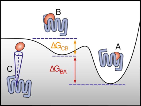
Schematic representation of the GPCR binding affinity calculation. A denotes the ligand-bound state, B a surface-exposed metastable state, and C a fully solvated state. The free-energy difference between B and the unbound reference state U is obtained by taking into account the conical restraint.

3.8 Calculation of the Binding Affinity

The overall binding affinity to the orthosteric or allosteric bound state A can be expressed as

$$K_A^{-1}=\frac{1}{[L]}\frac{p_U}{p_A}=\frac{1}{[L]}\frac{p_U}{p_B}\times \frac{p_B}{p_A}=K_B^{-1}\times \frac{p_B}{p_A}$$

where p_U is the probability of finding the ligand in the bulk solvent, p_A and p_B are the probabilities of the ligand bound in states A and B, respectively, and we have used the definition of binding affinity for state B. Using the expression for the latter calculated in the previous section, we obtain a final expression for the binding affinity to state A as follows:

$$K_A^{-1}=K_B^{-1}\times \text{exp}\left(-\frac{\mathrm{\Delta }{G}_{BA}}{k_{B}T}\right)$$

where ΔG_BA is the free-energy difference between states A and B.

References

- 1.Cherezov V, Abola E, Stevens RC. Recent progress in the structure determination of GPCRs, a membrane protein family with high potential as pharmaceutical targets. Methods Mol Biol. 2010;654:141–168. doi: 10.1007/978-1-60761-762-4_8. [DOI] [PMC free article] [PubMed] [Google Scholar]
- 2.Katritch V, Cherezov V, Stevens RC. Structure-function of the G protein-coupled receptor superfamily. Annu Rev Pharmacol Toxicol. 2013;53:531–556. doi: 10.1146/annurev-pharmtox-032112-135923. [DOI] [PMC free article] [PubMed] [Google Scholar]
- 3.Stevens RC, Cherezov V, Katritch V, Abagyan R, Kuhn P, Rosen H, Wuthrich K. The GPCR network: a large-scale collaboration to determine human GPCR structure and function. Nat Rev Drug Discov. 2013;12(1):25–34. doi: 10.1038/nrd3859. doi:10.1038/nrd3859, nrd3859 [pii] [DOI] [PMC free article] [PubMed] [Google Scholar]
- 4.Kruse AC, Ring AM, Manglik A, Hu J, Hu K, Eitel K, Hubner H, Pardon E, Valant C, Sexton PM, Christopoulos A, Felder CC, Gmeiner P, Steyaert J, Weis WI, Garcia KC, Wess J, Kobilka BK. Activation and allosteric modulation of a muscarinic acetylcholine receptor. Nature. 2013;504(7478):101–106. doi: 10.1038/nature12735. doi:10.1038/nature12735, nature12735 [pii] [DOI] [PMC free article] [PubMed] [Google Scholar]
- 5.Rasmussen SG, DeVree BT, Zou Y, Kruse AC, Chung KY, Kobilka TS, Thian FS, Chae PS, Pardon E, Calinski D, Mathiesen JM, Shah ST, Lyons JA, Caffrey M, Gellman SH, Steyaert J, Skiniotis G, Weis WI, Sunahara RK, Kobilka BK. Crystal structure of the beta2 adrenergic receptor-Gs protein complex. Nature. 2011;477(7366):549–555. doi: 10.1038/nature10361. doi:10.1038/nature10361, nature10361 [pii] [DOI] [PMC free article] [PubMed] [Google Scholar]
- 6.Kooistra AJ, Leurs R, de Esch IJ, de Graaf C. From three-dimensional GPCR structure to rational ligand discovery. Adv Exp Med Biol. 2014;796:129–157. doi: 10.1007/978-94-007-7423-0_7. [DOI] [PubMed] [Google Scholar]
- 7.Totrov M, Abagyan R. Flexible ligand docking to multiple receptor conformations: a practical alternative. Curr Opin Struct Biol. 2008;18(2):178–184. doi: 10.1016/j.sbi.2008.01.004. doi:10.1016/j.sbi.2008.01.004, S0959-440X(08)00008-0 [pii] [DOI] [PMC free article] [PubMed] [Google Scholar]
- 8.May A, Zacharias M. Protein-ligand docking accounting for receptor side chain and global flexibility in normal modes: evaluation on kinase inhibitor cross docking. J Med Chem. 2008;51(12):3499–3506. doi: 10.1021/jm800071v. [DOI] [PubMed] [Google Scholar]
- 9.Bowers KJ, Chow E, Xu H, Dror RO, Eastwood MP, Gregersen BA, Klepeis JL, Kolossvary I, Moraes MA, Sacerdoti FD, Salmon JK, Shan Y, Shaw DE. Scalable Algorithms for Molecular Dynamics Simulations on Commodity Clusters; Proceedings of the ACM/IEEE Conference on Supercomputing (SC06); Tampa, Florida. 11–17 November 2006.2006. [Google Scholar]
- 10.Van der Spoel D, Lindahl E, Hess B, Groenhof G, Mark AE, Berendsen HJC. GROMACS: fast, flexible, and free. J Comput Chem. 2005;26(16):1701–1718. doi: 10.1002/jcc.20291. [DOI] [PubMed] [Google Scholar]
- 11.Phillips JC, Braun R, Wang W, Gumbart J, Tajkhorshid E, Villa E, Chipot C, Skeel RD, Kale L, Schulten K. Scalable molecular dynamics with NAMD. J Comput Chem. 2005;26(16):1781–1802. doi: 10.1002/jcc.20289. [DOI] [PMC free article] [PubMed] [Google Scholar]
- 12.Fitch BG, Germain RS, Mendell M, Pitera J, Pitman M, Rayshubskiy A, Sham Y, Suits F, Swope W, Ward TJC, Zhestkov Y, Zhou R. Blue matter, an application framework for molecular simulation on Blue Gene. J Parallel Distrib Comput. 2003;63:759–773. doi: 10.1016/s0743-7315(03)00084-4. [DOI] [Google Scholar]
- 13.Shaw DE, Deneroff MM, Dror RO, Kuskin JS, Larson RH, Salmon JK, Young C, Batson B, Bowers KJ, Chao JC, Eastwood MP, Gagliardo J, Grossman JP, Ho CR, Ierardi DJ, Kolossvary I, Klepeis JL, Layman T, McLeavey C, Moraes MA, Mueller R, Priest EC, Shan YB, Spengler J, Theobald M, Towles B, Wang SC. Anton, a special-purpose machine for molecular dynamics simulation. Commun ACM. 2008;51(7):91–97. doi: 10.1145/1364782.1364802. [DOI] [Google Scholar]
- 14.Allen F, Almasi G, Andreoni W, Beece D, Berne BJ, Bright A, Brunheroto J, Cascaval C, Castanos J, Coteus P, Crumley P, Curioni A, Denneau M, Donath W, Eleftheriou M, Fitch B, Fleischer B, Georgiou CJ, Germain R, Giampapa M, Gresh D, Gupta M, Haring R, Ho H, Hochschild P, Hummel S, Jonas T, Lieber D, Martyna G, Maturu K, Moreira J, Newns D, Newton M, Philhower R, Picunko T, Pitera J, Pitman M, Rand R, Royyuru A, Salapura V, Sanomiya A, Shah R, Sham Y, Singh S, Snir M, Suits F, Swetz R, Swope WC, Vishnumurthy N, Ward TJC, Warren H, Zhou R, Team IBMBG Blue gene: a vision for protein science using a petaflop supercomputer. IBM Syst J. 2001;40(2):310–327. [Google Scholar]
- 15.Almasi G, Asaad S, Bellofatto RE, Bickford HR, Blumrich MA, Brezzo B, Bright AA, Brunheroto JR, Castanos JG, Chen D, Chiu GLT, Coteus PW, Dombrowa MB, Dozsa G, Eichenberger AE, Gara A, Giampapa ME, Giordano FP, Gunnels JA, Hall SA, Haring RA, Heidelberger P, Hoenicke D, Kochte M, Kopcsay GV, Kumar S, Lanzetta AP, Lieber D, Nathanson BJ, O’Brien K, Ohmacht AS, Ohmacht M, Rand RA, Salapura V, Sexton JC, Stemmacher-Burow BD, Stunkel C, Sugavanam K, Swetz RA, Takken T, Tian SR, Trager BM, Tremaine RB, Vranas P, Walkup RE, Wazlowski ME, Winograd S, Wisniewski RW, Wu P, Busche DR, Douskey SM, Ellavsky MR, Flynn WT, Germann PR, Hamilton MJ, Hehenberger L, Hruby BJ, Jeanson MJ, Kasemkhani F, Lembach RF, Liebsch TA, Lyndgaard KC, Lytle RW, Marcella JA, Marroquin CM, Mathiowetz CH, Maurice MD, Nelson E, Rickert DM, Sellers GW, Sheets JE, Strissel SA, Wait CD, Winter BB, Wood CJ, Zumbrunnen LM, Rangarajan M, Allen PV, Archer CJ, Blocksome M, Budnik TA, Ellis SD, Good MP, Gooding TM, Inglett TA, Kaliszewski KT, Knudson BL, Lappi C, Leckband GS, Lee S, Megerian MG, Miller SJ, Mundy MB, Musselman RG, Musta TE, Nelson MT, Obert CF, Van Oosten JL, Orbeck JP, Parker JJ, et al. Overview of the IBM Blue Gene/P project. IBM J Res Develop. 2008;52(1–2):199–220. [Google Scholar]
- 16.Dror RO, Pan AC, Arlow DH, Borhani DW, Maragakis P, Shan Y, Xu H, Shaw DE. Pathway and mechanism of drug binding to G-protein-coupled receptors. Proc Natl Acad Sci U S A. 2011;108(32):13118–13123. doi: 10.1073/pnas.1104614108. doi:10.1073/pnas.1104614108, 1104614108 [pii] [DOI] [PMC free article] [PubMed] [Google Scholar]
- 17.Kruse AC, Hu J, Pan AC, Arlow DH, Rosenbaum DM, Rosemond E, Green HF, Liu T, Chae PS, Dror RO, Shaw DE, Weis WI, Wess J, Kobilka BK. Structure and dynamics of the M3 muscarinic acetylcholine receptor. Nature. 2012;482(7386):552–556. doi: 10.1038/nature10867. doi:10.1038/nature10867, nature10867 [pii] [DOI] [PMC free article] [PubMed] [Google Scholar]
- 18.Dror RO, Green HF, Valant C, Borhani DW, Valcourt JR, Pan AC, Arlow DH, Canals M, Lane JR, Rahmani R, Baell JB, Sexton PM, Christopoulos A, Shaw DE. Structural basis for modulation of a G-protein-coupled receptor by allosteric drugs. Nature. 2013;503(7475):295–299. doi: 10.1038/nature12595. doi:10.1038/nature12595, nature12595 [pii] [DOI] [PubMed] [Google Scholar]
- 19.Laio A, Parrinello M. Escaping free-energy minima. Proc Natl Acad Sci U S A. 2002;99(20):12562–12566. doi: 10.1073/pnas.202427399. [DOI] [PMC free article] [PubMed] [Google Scholar]
- 20.Limongelli V, Bonomi M, Marinelli L, Gervasio FL, Cavalli A, Novellino E, Parrinello M. Molecular basis of cyclooxygenase enzymes (COXs) selective inhibition. Proc Natl Acad Sci U S A. 2010;107(12):5411–5416. doi: 10.1073/pnas.0913377107. doi:10.1073/pnas.0913377107, 0913377107 [pii] [DOI] [PMC free article] [PubMed] [Google Scholar]
- 21.Limongelli V, Marinelli L, Cosconati S, La Motta C, Sartini S, Mugnaini L, Da Settimo F, Novellino E, Parrinello M. Sampling protein motion and solvent effect during ligand binding. Proc Natl Acad Sci U S A. 2012;109(5):1467–1472. doi: 10.1073/pnas.1112181108. doi:10.1073/pnas.1112181108, 1112181108 [pii] [DOI] [PMC free article] [PubMed] [Google Scholar]
- 22.Grazioso G, Limongelli V, Branduardi D, Novellino E, De Micheli C, Cavalli A, Parrinello M. Investigating the mechanism of substrate uptake and release in the glutamate transporter homologue Glt(Ph) through meta-dynamics simulations. J Am Chem Soc. 2012;134(1):453–463. doi: 10.1021/ja208485w. [DOI] [PubMed] [Google Scholar]
- 23.Gervasio FL, Laio A, Parrinello M. Flexible docking in solution using metadynamics. J Am Chem Soc. 2005;127(8):2600–2607. doi: 10.1021/ja0445950. [DOI] [PubMed] [Google Scholar]
- 24.Provasi D, Bortolato A, Filizola M. Exploring molecular mechanisms of ligand recognition by opioid receptors with metadynamics. Biochemistry. 2009;48(42):10020–10029. doi: 10.1021/bi901494n. [DOI] [PMC free article] [PubMed] [Google Scholar]
- 25.Allen TW, Andersen OS, Roux B. Energetics of ion conduction through the gramicidin channel. Proc Natl Acad Sci U S A. 2004;101(1):117–122. doi: 10.1073/pnas.2635314100. [DOI] [PMC free article] [PubMed] [Google Scholar]
- 26.Roux B. Statistical mechanical equilibrium theory of selective ion channels. Biophys J. 1999;77(1):139–153. doi: 10.1016/S0006-3495(99)76878-5. [DOI] [PMC free article] [PubMed] [Google Scholar]
- 27.Rohl CA, Strauss CEM, Chivian D, Baker D. Modeling structurally variable regions in homologous proteins with rosetta. Proteins. 2004;55(3):656–677. doi: 10.1002/Prot10629. [DOI] [PubMed] [Google Scholar]
- 28.Fiser A, Sali A. MODELLER: generation and refinement of homology-based protein structure models. Methods Enzymol. 2003;374:461. doi: 10.1016/S0076-6879(03)74020-8. Macromolecular Crystallography, Pt D. [DOI] [PubMed] [Google Scholar]
- 29.Vanommeslaeghe K, MacKerell AD., Jr Automation of the CHARMM general force field (CGenFF) I: bond perception and atom typing. J Chem Inf Model. 2012;52(12):3144–3154. doi: 10.1021/ci300363c. [DOI] [PMC free article] [PubMed] [Google Scholar]
- 30.Vanommeslaeghe K, Raman EP, MacKerell AD., Jr Automation of the CHARMM general force field (CGenFF) II: assignment of bonded parameters and partial atomic charges. J Chem Inf Model. 2012;52(12):3155–3168. doi: 10.1021/ci3003649. [DOI] [PMC free article] [PubMed] [Google Scholar]
- 31.http://cgenff.paramchem.org/
- 32.Frisch MJ, Trucks GW, Schlegel HB, Scuseria GE, Robb MA, Cheeseman JR, Montgomery JAJ, Vreven T, Kudin KN, Burant JC, Millam JM, Iyengar SS, Tomasi J, Barone V, Mennucci B, Cossi M, Scalmani G, Rega N, Petersson GA, Nakatsuji H, Hada M, Ehara M, Toyota K, Fukuda R, Hasegawa J, Ishida M, Nakajima T, Honda Y, Kitao O, Nakai H, Klene M, Li X, Knox JE, Hratchian HP, Cross JB, Bakken V, Adamo C, Jaramillo J, Gomperts R, Stratmann RE, Yazyev O, Austin AJ, Cammi R, Pomelli C, Ochterski JW, Ayala PY, Morokuma K, Voth GA, Salvador P, Dannenberg JJ, Zakrzewski VG, Dapprich S, Daniels AD, Strain MC, Farkas O, Malick DK, Rabuck AD, Raghavachari K, Foresman JB, Ortiz JV, Cui Q, Baboul AG, Clifford S, Cioslowski J, Stefanov BB, Liu G, Liashenko A, Piskorz P, Komaromi I, Martin RL, Fox DJ, Keith T, Al-Laham MA, Peng CY, Nanayakkara A, Challacombe M, Gill PMW, Johnson B, Chen W, Wong MW, Gonzalez C, Pople JA. Gaussian 03, Revision C.02. Wallingford, CT: 2004. [Google Scholar]
- 33.Schrodinger L, New York, NY. Jaguar. version 7.6. 2009. [Google Scholar]
- 34.Kumar R, Iyer VG, Im W. CHARMM-GUI: a graphical user interface for the CHARMM users. Abstracts Papers Am Chem Soc. 2007;233:273. [Google Scholar]
- 35.Wu EL, Cheng X, Jo S, Rui H, Song KC, Davila-Contreras EM, Qi YF, Lee JM, Monje-Galvan V, Venable RM, Klauda JB, Im W. CHARMM-GUI Membrane Builder Toward Realistic Biological Membrane Simulations. J Comput Chem. 2014;35(27):1997–2004. doi: 10.1002/Jcc.23702. [DOI] [PMC free article] [PubMed] [Google Scholar]
- 36.http://www.charmm-gui.org/
- 37.Kandt C, Ash WL, Tieleman DP. Setting up and running molecular dynamics simulations of membrane proteins. Methods. 2007;41(4):475–488. doi: 10.1016/j.ymeth.2006.08.006. [DOI] [PubMed] [Google Scholar]
- 38.Schmidt TH, Kandt C. LAMBADA and InflateGRO2: efficient membrane alignment and insertion of membrane proteins for molecular dynamics simulations. J Chem Inform Model. 2012;10:2657–2669. doi: 10.1021/ci3000453. [DOI] [PubMed] [Google Scholar]
- 39.Hess B, Kutzner, van der Spoel D, Lindahl E. GROMACS 4: algorithms for highly efficient, load-balanced, and scalable molecular simulation. J Chem Theory Comput. 2008;4(3):435–447. doi: 10.1021/ct700301q. [DOI] [PubMed] [Google Scholar]
- 40.Bonomi M, Branduardi D, Bussi G, Camilloni C, Provasi D, Raiteri P, Donadio D, Marinelli F, Pietrucci F, Broglia RA, Parrinello M. PLUMED: a portable plugin for free-energy calculations with molecular dynamics. Comput Phys Commun. 2009;180(10):1961–1972. [Google Scholar]
- 41.Humphrey W, Dalke A, Schulten K. VMD: visual molecular dynamics. J Mol Graphics. 1996;14:33–38. doi: 10.1016/0263-7855(96)00018-5. [DOI] [PubMed] [Google Scholar]
- 42.DeLano WL. The PyMOL molecular graphics system. DeLano Scientific; San Carlos, CA: 2002. [Google Scholar]
- 43.http://zhanglab.ccmb.med.umich.edu/GPCR-EXP/
- 44.Fiser A, Do RKG, Sali A. Modeling of loops in protein structures. Protein Sci. 2000;9(9):1753–1773. doi: 10.1110/ps.9.9.1753. [DOI] [PMC free article] [PubMed] [Google Scholar]
- 45.Mandell DJ, Coutsias EA, Kortemme T. Sub-angstrom accuracy in protein loop reconstruction by robotics-inspired conformational sampling. Nat Methods. 2009;6(8):551–552. doi: 10.1038/nmeth0809-551. [DOI] [PMC free article] [PubMed] [Google Scholar]
- 46.Morris GM, Huey R, Lindstrom W, Sanner MF, Belew RK, Goodsell DS, Olson AJ. AutoDock4 and AutoDockTools4: automated docking with selective receptor flexibility. J Comput Chem. 2009;30(16):2785–2791. doi: 10.1002/Jcc.21256. [DOI] [PMC free article] [PubMed] [Google Scholar]
- 47.Mysinger MM, Shoichet BK. Rapid context-dependent ligand desolvation in molecular docking. J Chem Inform Model. 2010;50(9):1561–1573. doi: 10.1021/Ci100214a. [DOI] [PubMed] [Google Scholar]
- 48.Brooks BR, Bruccoleri RE, Olafson BD, States DJ, Swaminathan S, Karplus M. CHARMM: a program for macromolecular energy, minimization, and dynamics calculations. J Comput Chem. 1983;4(2):187–217. [Google Scholar]
- 49.Foloppe N, MacKerell AD. All-atom empirical force field for nucleic acids: I. Parameter optimization based on small molecule and condensed phase macromolecular target data. J Comput Chem. 2000;21(2):86–104. doi: 10.1002/(Sici)1096-987x(20000130)21:2<86::Aid-Jcc2>3.0.Co;2-G. [DOI] [Google Scholar]
- 50.http://mackerell.umaryland.edu/charmm_ff.shtml
- 51.Bussi G, Donadio D, Parrinello M. Canonical sampling through velocity rescaling. J Chem Phys. 2007;126(1):Artn014101. doi: 10.1063/1.2408420. [DOI] [PubMed] [Google Scholar]
- 52.Parrinello M, Rahman A. Polymorphic transitions in single-crystals: a new molecular-dynamics method. J Appl Phys. 1981;52(12):7182–7190. doi: 10.1063/1.328693. [DOI] [Google Scholar]
- 53.Barducci A, Bonomi M, Parrinello M. Metadynamics. Wiley Interdisciplinary Reviews. Comput Mol Sci. 2011;1(5):826–843. doi: 10.1002/Wcms.31. [DOI] [Google Scholar]
- 54.Raiteri P, Laio A, Gervasio FL, Micheletti C, Parrinello M. Efficient reconstruction of complex free energy landscapes by multiple walkers metadynamics. J Phys Chem B. 2006;110(8):3533–3539. doi: 10.1021/Jp054359r. [DOI] [PubMed] [Google Scholar]
- 55.Sutto L, D’Abramo M, Gervasio FL. Comparing the efficiency of biased and unbiased molecular dynamics in reconstructing the free energy landscape of met-enkephalin. J Chem Theor Comput. 2010;6:3640–3646. [Google Scholar]
- 56.Berendsen HJC, Vanderspoel D, Vandrunen R. Gromacs: a message-passing parallel molecular-dynamics implementation. Comput Phys Commun. 1995;91(1–3):43–56. doi: 10.1016/0010-4655(95)00042-E. [DOI] [Google Scholar]
- 57.Case DA, Cheatham TE, Darden T, Gohlke H, Luo R, Merz KM, Onufriev A, Simmerling C, Wang B, Woods RJ. The Amber biomo-lecular simulation programs. J Comput Chem. 2005;26(16):1668–1688. doi: 10.1002/Jcc.20290. [DOI] [PMC free article] [PubMed] [Google Scholar]
- 58.Pearlman DA, Case DA, Caldwell JW, Ross WS, Cheatham TE, Debolt S, Ferguson D, Seibel G, Kollman P. Amber, a package of computer-programs for applying molecular mechanics, normal-mode analysis, molecular-dynamics and free-energy calculations to simulate the structural and energetic properties of molecules. Comput Phys Commun. 1995;91(1–3):1–41. doi: 10.1016/0010-4655(95)00041-D. [DOI] [Google Scholar]
- 59.Tribello GA, Bonomi M, Branduardi D, Camilloni C, Bussi G. PLUMED 2: new feathers for an old bird. Comput Phys Commun. 2014;185(2):604–613. doi: 10.1016/j.cpc.2013.09.018. [DOI] [Google Scholar]
- 60.Costanzi S, Wang KY. The GPCR crystallography boom: providing an invaluable source of structural information and expanding the scope of homology modeling. G Protein-Coupled Receptors. Model Simulat. 2014;796:3–13. doi: 10.1007/978-94-007-7423-0_1. [DOI] [PubMed] [Google Scholar]
- 61.Sandal M, Duy TP, Cona M, Zung H, Carloni P, Musiani F, Giorgetti A. GOMoDo: a GPCRs online modeling and docking web-server. Plos One. 2013;8(9):e74092. doi: 10.1371/journal.pone.0074092. [DOI] [PMC free article] [PubMed] [Google Scholar]
- 62.Yoshikawa Y, Oishi S, Kubo T, Tanahara N, Fujii N, Furuya T. Optimized method of G-protein-coupled receptor homology modeling: its application to the discovery of Novel CXCR7 ligands. J Med Chem. 2013;56(11):4236–4251. doi: 10.1021/Jm400307y. [DOI] [PubMed] [Google Scholar]
- 63.Vanommeslaeghe K, Hatcher E, Acharya C, Kundu S, Zhong S, Shim J, Darian E, Guvench O, Lopes P, Vorobyov I, Mackerell AD., Jr CHARMM general force field: a force field for drug-like molecules compatible with the CHARMM all-atom additive biological force fields. J Comput Chem. 2010;31(4):671–690. doi: 10.1002/jcc.21367. [DOI] [PMC free article] [PubMed] [Google Scholar]
- 64.http://www.msg.ameslab.gov/gamess/capabilities.html
- 65.http://www.abinit.org
- 66.Laio A, Rodriguez-Fortea A, Gervasio FL, Ceccarelli M, Parrinello M. Assessing the accuracy of metadynamics. J Phys Chem B. 2005;109(14):6714–6721. doi: 10.1021/jp045424k. [DOI] [PubMed] [Google Scholar]