Abstract
The viscoelastic behaviour of a biological material is central to its functioning and is an indicator of its health. The Fung quasi-linear viscoelastic (QLV) model, a standard tool for characterizing biological materials, provides excellent fits to most stress–relaxation data by imposing a simple form upon a material's temporal relaxation spectrum. However, model identification is challenging because the Fung QLV model's ‘box’-shaped relaxation spectrum, predominant in biomechanics applications, can provide an excellent fit even when it is not a reasonable representation of a material's relaxation spectrum. Here, we present a robust and simple discrete approach for identifying a material's temporal relaxation spectrum from stress–relaxation data in an unbiased way. Our ‘discrete QLV’ (DQLV) approach identifies ranges of time constants over which the Fung QLV model's typical box spectrum provides an accurate representation of a particular material's temporal relaxation spectrum, and is effective at providing a fit to this model. The DQLV spectrum also reveals when other forms or discrete time constants are more suitable than a box spectrum. After validating the approach against idealized and noisy data, we applied the methods to analyse medial collateral ligament stress–relaxation data and identify the strengths and weaknesses of an optimal Fung QLV fit.
Keywords: quasi-linear viscoelasticity, spectral analysis, stress–relaxation, ligament
1. Introduction
The Fung quasi-linear viscoelastic (QLV) model is a standard tool for representing the nonlinear history- and time-dependent soft-tissue viscoelasticity of biological tissues [1–4]. The QLV model provides a simple fit to stress–relaxation tests, which are preferred over standard rotational rheometry for biological tissues due to issues of gripping and anisotropy. These tests involve stretching a specimen a prescribed amount and then analysing the relaxation over time of the force needed to sustain this level of stretch. However, the confidence interval for estimation of the parameters of the ‘box’-shaped temporal relaxation function that Fung suggested in his book [1] are typically large [5], which complicates comparison of materials. Further, the usual box form of the temporal relaxation function is sufficiently restrictive that many have found the need to apply different relaxation functions [6–8] or apply different QLV representations altogether [9]. Finally, identifying when the box spectrum is too restrictive to describe a specific biological material's time-dependent mechanical responses is a challenge [3,10–17] because, with this box spectrum, the Fung QLV model can fit relaxation data even for materials whose responses to dynamic loading it would fail to predict [18,19].
We present here a simple technique to overcome these challenges. The core of the technique is a finite series that, under special conditions, reduces to Fung's box spectrum relaxation function.
In this article, we show that application of our discrete QLV (DQLV) form of the Fung QLV model is a simple and effective way to identify material relaxation spectra in an unbiased manner from stress–relaxation data. The approach identifies ranges of time constants over which Fung's continuous box relaxation spectrum is appropriate, and is effective at fitting this box relaxation spectrum. It also identifies when discrete time constants are more appropriate than the box relaxation spectrum for representing damping responses. After presenting the DQLV model, we apply it to correctly identify spectra at particular strain levels from simple relaxation tests, and then demonstrate its utility on determining the quasi-viscoelastic response of the rabbit medial collateral ligament (MCL).
2. Background
We begin with an overview of the integral form of linear and QLV models with the goal of setting the stage for the specific discrete relaxation function we present in §3.
2.1. Integral form of linear viscoelasticity
The behaviour of a linear viscoelastic material in one dimension can be represented by the following convolution integral [20,21]:
| 2.1 |
where ψ(t, u) is a material modulus function, t is time, σ is engineering stress and ɛ is linearized strain. For hereditary or non-ageing materials, this reduces to
| 2.2 |
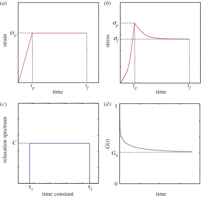
where the relaxation function φ(t) describes the mechanical character of a material, ranging from an elastic solid (φ = const.) to a Newtonian fluid (φ(t) = ηδ(t), where η is a coefficient of viscosity and δ(t) is Dirac's delta function. For a material with both elastic and viscous properties, φ(t) must be a generalized function that defines the whole spectrum of material behaviour. Here φ(t) is determined in general by fitting to data from an experiment such as a stress–relaxation test, in which a sample is subjected to a linear ramp at strain rate  over time 0 ≤ t ≤ tp, followed by an isometric relaxation phase over tp ≤ t ≤ tf (figure 1a,b).
Figure 1.
Characterization of a viscoelastic material through a standard ramp-and-hold test. (a) In a ramp-and-hold relaxation test, uniaxial strain is increased at a constant rate  over a time tp then held at an isometric level
  until time tf. (b) In response, the stress varies with time, rising to a peak value σp and then relaxing to a value σf. (c) For biological tissues, such data are often interpreted using Fung's QLV theory, involving a box-shaped relaxation spectrum of height C. (d) The parameters describing this box spectrum can be rearranged to predict the ‘reduced relaxation function’ that appears in the Fung QLV constitutive law. (Online version in colour.)
2.2. Fung's quasi-linear viscoelastic model
In a biological material, φ(t) is typically inadequate because the relaxation function depends upon the degree to which the material is strained. Fung's QLV model, reviewed extensively and in more detail by others [7,8,12,14,15,18,22–27], provides a simple strain-dependent extension of (2.2) in which the temporal decay of stress is independent of strain:
| 2.3 |
where G(t) is a normalized function of time so that  (time-independent component of G) and
  (figure 1d); K(ɛ,t) represents stress and σ(e)(ɛ) represents the elastic response. Based upon the concave-up force–displacement curves common to collagenous tissues, Fung proposed using an exponential relationship that he attributes to Kenedi et al. [1,28], for the elastic stress component:
| 2.4 |
The stress responses to a small strain increment, applied at time u, G(t − u) (∂σ(e)(ɛ))/(∂ɛ) δɛ(u), can be summed using the Boltzmann superposition principle, so that the stress for t ≥ 0 can be written as
| 2.5 |
where G(t) is a monotonically decreasing function [21]; as in the fading memory model, the recent strain history determines material response. Fung termed G(t) the ‘reduced relaxation function’ and suggested the form
 |
2.6 |
where S(τ) is the following function, first proposed independently by others including Neubert [29]:
 |
2.7 |
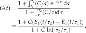
in which C, τ1 and τ2 are material constants to be determined experimentally (figure 1c). Substituting, one arrives at the form that is ubiquitous in the biomechanics literature:
 |
2.8 |
where  is the exponential integral function. This version of the Fung QLV model is predicated upon the requirements of equations (2.3), (2.4) and (2.7). Although the typical implementation focuses on small strain applications, straightforward extensions of the Fung QLV model to finite strain exist [30–32]. However, the suitability of the assumption of equation (2.3) must be checked carefully for any material to which these extensions are applied.
In §3, we present a simple tool to identify whether the relaxation response S(τ) follows the box spectrum of equation (2.7), and whether this response is independent of strain (cf. equation (2.3)). We further propose a simple technique for modelling a material if these requirements prove unsuitable.
2.3. Schematic of the Fung quasi-linear viscoelastic model
Two graphical representations of the Fung QLV model should be mentioned. These provide a foundation for interpreting the fitting and model identification tools presented in §3.
2.3.1. Standard linear solid models in series
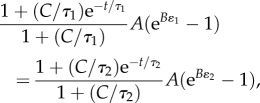
The Fung QLV model can be represented as an infinite number of standard linear solid elements in series, modified so that linear springs are replaced by nonlinear springs (figure 2a). S(τ) for each of those elements varies between two constants: S(τ2) < C/τ < S(τ1). Noting that the stress in each element is equal, a relationship can be written between the first and the last elements:
 |
2.9 |
where A, B, C, τ1 and τ2 are the five QLV parameters to be fit. The first element (S = C/τ1) has the highest strain, ɛ1, while the last (S = C/τ2) has the smallest, ɛ2. Equation (2.9) shows a major difference between the QLV and generalized Maxwell models [33]. Because the viscoelastic elements in the QLV model are in series, changing τ1 or τ2 changes the stress in all of the individual models (figure 2a). Thus, in contrast to the generalized Maxwell model, τ1 and τ2 are not the fastest and slowest viscoelastic time constants, respectively. Rather, they are time-domain parameters whose values affect the entire stress–relaxation curve.
Figure 2.
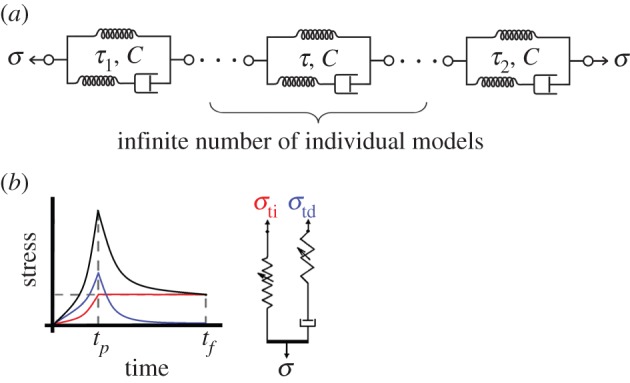
Schematic of the Fung box spectrum model. (a) The box spectrum model can be represented schematically by a continuous series of nonlinear viscoelastic elements, each associated with a time constant between the limits τ1 and τ2 of the box relaxation spectrum, and with the height C of the box relaxation spectrum (cf. figure 1). (b) In another representation, with a different type of nonlinear spring, the time-independent and -dependent stress responses can be separated as in equation (2.12). (Online version in colour.)
2.3.2. Temporal quasi-linear viscoelastic decomposition
A second useful schematic depiction of the Fung QLV model involves decomposition into time-independent and -dependent parts. This decomposition is instructive and useful, because it introduces a constraint upon the five QLV parameters. Following a ramp to a sustained level of isometric stretch (cf. figure 1a), the relaxation function, G(t), (t > tp) is
 |
2.10 |
where Gti represents the time-independent and Gtd the time-dependent parts of the reduced relaxation function. The stress can likewise be separated into time-independent and -dependent parts (figure 2b).
For example, for a specimen that is fully relaxed at time t = 0 and is stretched at a constant strain rate  from t = 0 to tp then held isometrically until t = tf (figure 1a),
 |
2.11 |
or
| 2.12 |
Schematically, the first term on the right-hand side of these equations represents the stress in a nonlinear time-independent (strain-dependent) spring, and the second term represents a nonlinear spring, with linear viscous damping, which is time-dependent (figure 2b). After sufficient relaxation, the second term on the right-hand side of equation (2.11) or equation (2.12) approaches 0, and σ(t) approaches a steady state:
| 2.13 |
where  Thus, a way to ensure that the five QLV parameters are estimated correctly from a dataset is to compare the stress asymptote in the data to
  from equation (2.13) (figure 1b), assuming the isometric portion of the experiment was sufficiently long to provide an accurate estimate of σ(∞).
3. Methods
3.1. Continuous quasi-linear viscoelastic spectrum
To analyse a material's relaxation spectrum without any specific pre-assumption for S(τ), suppose S(τ) is
 |
3.1 |
where, for h(τ) = C, equation (3.1) reduces to the Fung QLV model (cf. equation (2.7)). Plugging equation (3.1) into equation (2.6), the relaxation function can be written as
 |
3.2 |
Then, for a fully relaxed specimen stretched at a constant strain rate  over the time interval 0 to tp and held isometrically until time tf, the stress history can be written as
 |
3.3 |
In the above equations, A, B, h(τ), τmin and τmax are unknowns that should be estimated by fitting σ(t) to experimental stress–relaxation data. This, unfortunately, is an ill-posed problem. However, a broad range of techniques exists to find a solution [21,34–36] that is suitable and repeatable, if not unique.
3.2. Discrete quasi-linear viscoelastic spectrum
A discretization technique simplifies this ill-posed problem. Although several approaches exist for discretizing viscoelastic responses, including the Prony series approach, our specific objective is to arrive at an approach that yields a graphical representation to easily identify the suitability of the Fung box spectrum over a particular range of loading conditions.
The approach we take begins with a discrete form of the integral  with the interval (λ1, λn+1) divided into n equidistant logarithmic subintervals
 |
3.4 |
For the case of λi distributed equidistantly over the range λ1 ≤ λi ≤ λn, one can further simplify to write
 |
3.5 |
where the constant  and Hi is the height of the ith rectangle and τi is the corresponding time constant (figure 3). The spectrum Hi(τi) represents a tool for model identification, which we term a ‘DQLV’ spectrum, which simplifies to the continuous Fung box spectrum when appropriate. Throughout, we use the superscript DQLV to distinguish parameters arising from a DQLV fitting from those arising from a box spectrum fitting. The discrete form of equation (3.2) is
| 3.6 |
Figure 3.
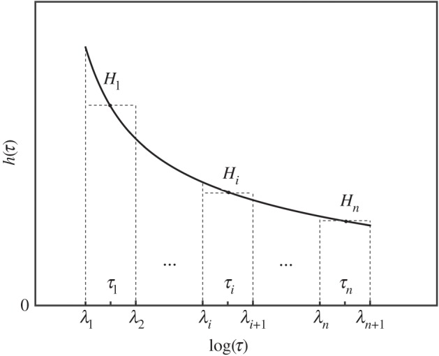
Schematic of the discretization of the continuous function h(τ). A partition of an interval [λ1, λn+1] is a finite sequence of n subintervals on a logarithmic x-axis. [λi, λi+1] is the width and Hi is the height of the ith rectangle and τi time constant corresponding to Hi.
and that of equation (3.1) is
 |
3.7 |
where Hi are parameters to be fit and τ1 and τn, as described below, are chosen to encompass a range broader than that needed to describe a material. In contrast to the Neubert [29] and Fung box spectrum models [1], the values of Hi need not be identical. Schematically, the DQLV model is analogous to the box spectrum model, except with a finite number of elements, Hi, that represent the relaxation spectrum (figure 4). For materials that are not well fit by the box spectrum model, the insertion of equation (3.7) into equation (2.6) provides for a simple extension of the QLV model. We note that, although the DQLV spectrum reduces to a box spectrum, it is different in that the values of Hi need not be constant. Further, although this physical meaning of τ1 and τn is analogous to these constants within a Prony series, we note that the DQLV spectrum reduces to a box spectrum when a box spectrum is indeed the correct representation of a material's relaxation response. The model does not reduce to the spectral representation that would be obtained using the generalized Maxwell model [37].
Figure 4.
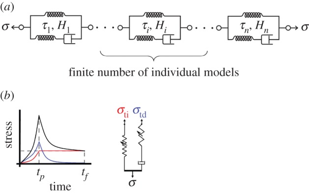
The DQLV model differs from the Fung box spectrum model in that it has a finite number n of elements analogous to those in figure 2a, each with a discrete time constant τi and with a potentially different height Hi. (b) The time-independent and -dependent stress responses can be separated as in figure 2b. (Online version in colour.)
3.3. Numerical fitting algorithms
As in equation (2.10), we can split G(DQLV)(t) into time-independent and -dependent parts:
 |
3.8 |
Because of the nature of ill-posed problems, we expect predictions to show some deviation from a Fung box spectrum even for artificial data generated from the Fung model [36,38–40]. Thus, we used a simple regularizing criterion, which acted as a penalty against unwanted states and ensured that the fitting algorithm did not become trapped in local minima. In this approach, Hi were smoothed by a regularization function and were identified by minimizing
 |
3.9 |
where f is the number of data points,  are known stress data or a calculable relationship and α is a regulating factor. Parameters were determined using a non-negative least-squares regression [41]. For any α of the order of 1, the parameter estimates were insensitive to the specific choice of α. α = 1 was used in the model validation studies below.
  are DQLV estimates of
  :
:
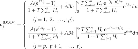 |
3.10 |
where p and f are the number of data points in ramp and relaxation intervals, respectively.
3.4. Validation of software to estimate discrete quasi-linear viscoelastic spectra
A code to obtain the DQLV spectrum of a material from stress versus time data in a relaxation test was generated in the Matlab environment. The code is available from the authors.
Because the DQLV model represents an approximation of the real spectrum of a material [36], it was important to validate the model and check the reproducibility of the approximation. Validations were performed by using the DQLV model to fit stress–relaxation data generated using either the Fung QLV model with a box spectrum or using the generalized Maxwell model, the latter having three time constants (including the infinite time constant; e.g. [42,43]).
The stability of the model with respect to noise was then studied. Random noise was added to the simulated Fung QLV stress–relaxation data to evaluate how noise affects DQLV analysis results. We superimposed upon the data noise chosen from a uniform distribution with amplitudes of 5, 10, 15, 20 or 25% of the steady-state stress. Fifty noisy datasets were generated (10 sets for each noise percentage). Relaxation spectra, H(τ), for these new datasets were estimated using the DQLV approach. The sensitivity to noise level was then quantified by the mean square error (MSE) of the predicted stress–relaxation compared to the underlying input stress–relaxation data.
3.5. Characterization of medial collateral ligament relaxation
As an example of DQLV characterization of an orthopedic tissue, we studied either the left or the right MCL from N = 6 skeletally mature female New Zealand white rabbits. Prior to dissection, knees were wrapped in saline-soaked gauze and then sealed in plastic bags and fresh frozen at −20°C [44]. On the day of testing, knees were thawed to room temperature and MCLs were dissected and cut free at the insertion sites [45,46]. The geometry was standardized by cutting the ligaments into dog bone shapes with a length-to-width ratio of 6.8 ± 0.8 (width 1.6 ± 0.2 mm). The tissue samples were fixed in custom-made soft-tissue clamps, and the cross-sectional area was determined with a laser micrometer system (1.0 ± 0.3 mm2) [44,47]. Measurements were taken in three locations along the length of the tissue sample and averaged for stress calculations. The tissue sample–clamp construct was then mounted to a tensile testing machine (Enduratec Elf 3200, Bose Corporation, Framingham, MA, USA). Reflective markers were placed on the tissue sample to track strain using an optical system (VP110, Motion Analysis, Santa Rosa, CA, USA). A saline drip was used to hydrate the tissue sample and maintain temperature at a constant 37°C. The tissue sample was aligned along the loading axis using an x–y table and then was left unloaded for 30 min to acclimate. Specimens were elongated to strain levels of 1.25, 2.5 and 5% and held isometrically at each level for 35 min to reach equilibrium [48]. Force data were acquired at 3 Hz throughout the ramp and 35 min relaxation intervals. The ramp time for all three samples was approximately 9.2 s; thus, the specimens' strain rates were approximately 0.135% s–1, approximately 0.271% s–1 and approximately 0.543% s–1, respectively. The experimental data were fit using both the DQLV and Fung box spectrum models [5].
4. Results and discussion
4.1. Fitting of simulated data
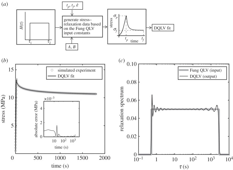
In the first validation study, stress–relaxation data were calculated for a Fung QLV material whose relaxation response followed a box spectrum, and the DQLV model was applied to estimate the parameters used to generate these data. The parameters chosen were those reported by Abramowitch et al. [5] for a goat MCL that was strained to 2.76% over 18.4 s and then held isometrically for 3600 s (figure 5a,b and table 1). The DQLV model was applied using equation (3.10), which constrains the DQLV model to fit stress–relaxation data. A spectrum that approximated a box spectrum was predicted, indicating that the material would be well modelled by a box spectrum representation. Several sets of time constants and different regularization parameters α were evaluated to ensure that the DQLV spectrum was repeatable. The predicted spectra were insensitive to the choice of α for α of the order of 1, and α = 1 was adopted for all subsequent analyses. The spectrum shown in figure 5c had n = 100 time constants. Increasing n provided a better quantitative fit to the stress–relaxation data, but did not change the qualitative nature of the predicted DQLV spectrum.
Figure 5.
Validation of the DQLV fitting method against simulated stress–relaxation data from an ideal Fung QLV material with a box spectrum. (a) Simulated stress–relaxation data were generated for an idealized Fung QLV material with a box spectrum, then fit with the DQLV model. (b) DQLV fitting provided and excellent fit to the input data. (c) The DQLV spectrum approximated a box-shape.
Table 1.
Constants describing the parameters of reduced relaxation function, the instantaneous elastic response and the strain profile for goat MCL [5].
| A (MPa) | B | C | τ1 (s) | τ2 (s) | tp (s) | tf (s) |  |
|---|---|---|---|---|---|---|---|
| 32.86 | 13.5 | 0.05 | 0.51 | 2786 | 18.4 | 3618.4 | 0.0015 |
An interesting feature of the DQLV analysis is that the predicted DQLV spectrum, despite its deviation from a box shape, yielded error of less than 0.01% of the peak stress when predicting stress–relaxation data generated using a flat box spectrum. Indeed, the Fung box spectrum and DQLV fits were both indistinguishable from the input relaxation data (figure 5c). The logical course of action for a DQLV spectrum such as this would thus be to adopt the simpler box spectrum fitting for subsequent analysis of this material.
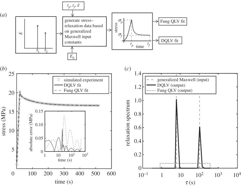
We next studied whether the DQLV model could identify when stress–relaxation data should not be represented by a Fung box spectrum. The input data in this case were generated using a generalized Maxwell model [33] including two Maxwell elements in addition to a linear spring, all acting in parallel. The data chosen were those reported by Shen et al. [49] for fitting the response of a sea cucumber (Cucumaria frondosa) collagen fibril following a 20 s ramp to a strain of 20% and a subsequent 520 s isometric hold (figure 6a,b and table 2). The DQLV fitting recovered a Maxwell-type spectrum with two distinct peaks at the two non-infinite time constants used to generate the input data (figure 6c).
Figure 6.
Validation of the DQLV fitting method to simulated stress–relaxation data from an ideal generalized Maxwell material. (a) Simulated stress–relaxation data were generated for an ideal generalized Maxwell model with two time constants, then fit with the DQLV model. (c) The DQLV spectrum identified the two discrete time constants accurately. (b) Despite the inappropriateness of a Fung box spectral fitting, both fittings provided excellent fits to the input data.
Table 2.
Constants describing the elastic moduli, the relaxation time constants and the strain profile for isolated collagen fibrils of Cucumaria frondosa [42].
| E0 (MPa) | E1 (MPa) | E2 (MPa) | τ1 (s) | τ2 (s) | tp (s) | tf (s) |  |
|---|---|---|---|---|---|---|---|
| 83 × 106 | 19 × 106 | 14 × 106 | 6 | 100 | 20 | 520 | 0.0100 |
However, the box spectrum fitting (figure 6c), also yielded an excellent fit to the stress–relaxation data. The fitting error, as observed in the plot of the residuals (inset of figure 6b), was only slightly higher than that of the DQLV fitting. This very small difference in residual error highlights the peril of fitting a Fung QLV box spectrum in the absence of a spectral evaluation such as that which the DQLV model provides: although the box spectrum model captured the relaxation data very well, this prediction captures the frequency dependence of the material response very poorly at the extremes of the range of time constants [18,19]. As we emphasize in the sequel to this article, the errors become substantial when attempting to predict material response under dynamic loading.
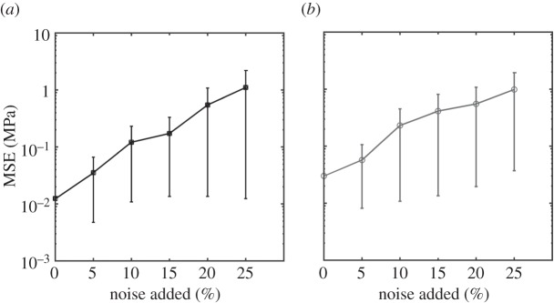
Finally, the fittings were remarkably robust against Gaussian random noise for both the DQLV (figure 7a) and box spectrum (figure 7b) models. MSEs increased with noise, but were less than 2 MPa for 25% noise in both models, compared to a peak stress of about 13 MPa.
Figure 7.
Assessment of the susceptibility of the DQLV and Fung QLV fitting methods to experimental noise. (a) DQLV and (b) Fung QLV fittings of simulated data reproduced the stress–relaxation curves in a way that was robust against noise. The DQLV model showed lower MSE than the Fung QLV model. Shown is the mean squared error (MSE) of the fit to the stress–relaxation data for fitting of 10 different noisy sets of relaxation data at each of five different levels of noise. For comparison, the peak stress was about 13 MPa. Noise was introduced by adding a Gaussian random fraction of the quantity β(σf) to each data point, where  .
.
4.2. Discrete quasi-linear viscoelastic fitting of stress–relaxation data of rabbit medial collateral ligament
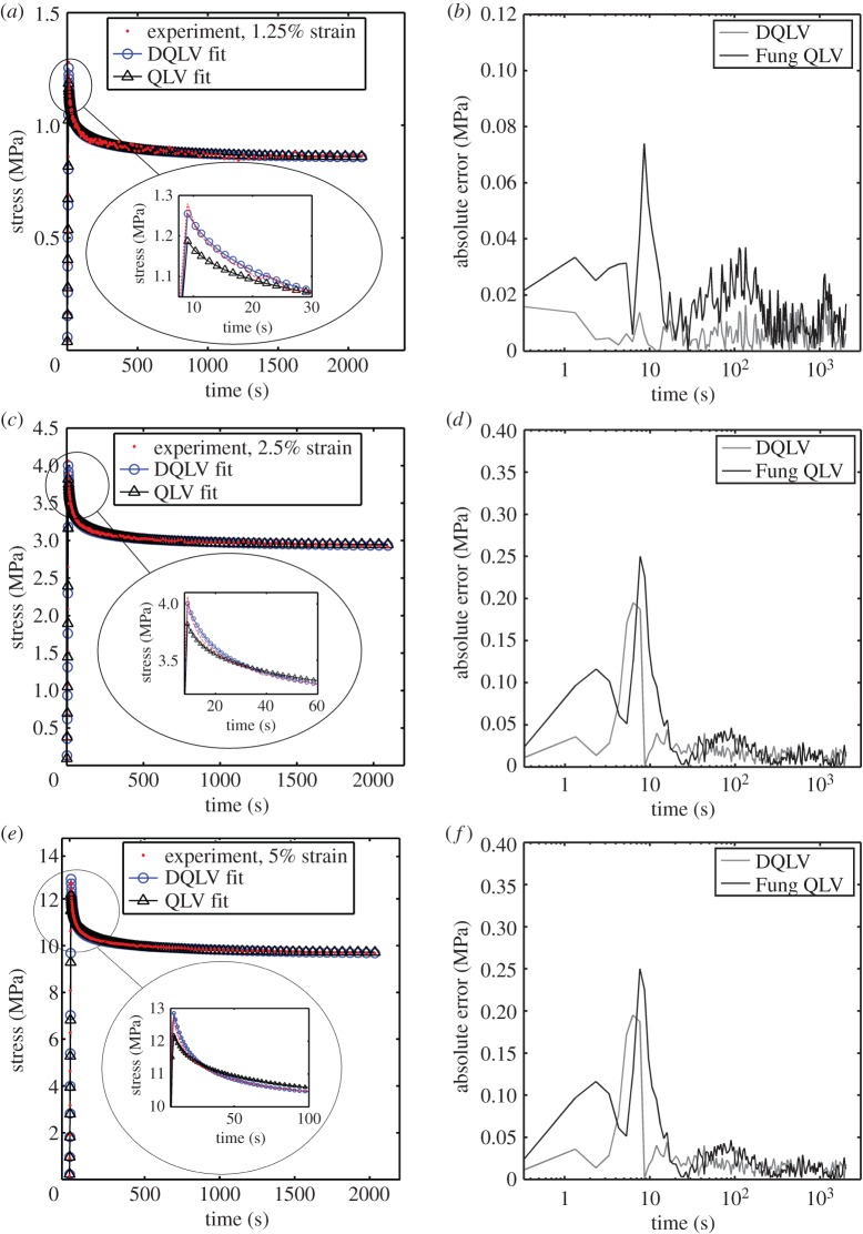
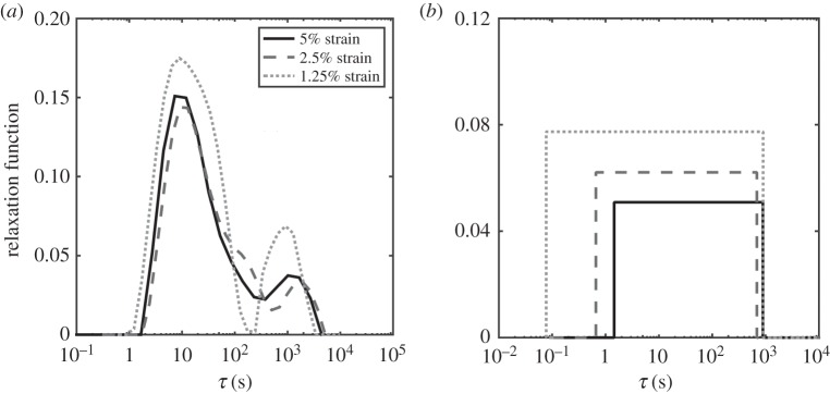
The stress–relaxation data for rabbit MCLs at strain levels of 1.25, 2.5 and 5% all showed a characteristic rise during stretching, then gradually decreased to plateau at about 2000 s (figure 8a,c,e). Both the DQLV and box spectrum models fit the experimental data with acceptable error, but the DQLV had higher precision (figure 8b,d,f). By comparing the DQLV spectra (figure 9a) to the Fung box spectra (figure 9b) of the three stress–relaxation tests, it is clear that the box spectra weakly estimated the lower boundary of dominant time constants of the system. The DQLV model estimation, on the other hand, was more consistent. Moreover, the DQLV model illuminated a structurally fast time constant at about 10 s and a slow time constant at about 1000 s that were not detectable by the Fung box spectra. These observations are consistent with dynamic testing reported for other tissues [18,19,50].
Figure 8.
Demonstration of the fitting methods on experimental stress–relaxation data from a ligament. DQLV and Fung QLV fittings of stress–relaxation data acquired from a rabbit MCL stretched to (a) 1.25, (c) 2.5 and (e) 5% strain. The residuals were substantially lower for the DQLV fittings at all three strain levels: (b) 1.25, (d) 2.5 and (f) 5% strain. (Online version in colour.)
Figure 9.
DQLV and Fung QLV spectra of the rabbit MCL. (a) The DQLV spectra were very similar at all three strain levels, which is a fundamental requirement for using the Fung QLV model. However, the spectra showed two dominant peaks (around 10 s and around 1000 s) rather than a box spectrum, which precludes use of the Fung QLV model. (b) The Fung QLV model produced a poor fit to this spectrum, with the lower range of τ mispredicted and the minor variations of the spectrum with respect to strain exaggerated.
The DQLV spectrum showed reasonable repeatability for the three strain levels, suggesting that the Fung QLV model's criterion of a strain-independent reduced relaxation function would be met reasonably well for the rabbit MCL specimens tested. However, the other condition, that of a flat, box-like spectrum was not met: the continuous spectrum of equation (3.1) must have constant dimensionless height h(τ) = C over some range of τ1–τ2, but the values of τ1,τ2 and C varied substantially for the best fits to the three tests. Errors associated with applying the box spectrum model become evident at the lower boundary of the time constants (figure 9b).
4.3. Choosing among models
For a tissue such as the rabbit MCL studied above, a more detailed description of the spectrum would be required, especially under dynamic loading. Two logical choices are a normalized, generalized form of the Maxwell model and the DQLV model. Both are related in that they involve a Prony series, and both have strengths and limitations.
The generalized Maxwell model is an excellent tool for fitting most experimental stress–relaxation data, and can usually do so with only two or three exponential terms [37]. This is a strength because of its simplicity, but is also a limitation because the limited number of time constants may be inadequate to reveal either the range of relaxation mechanisms or the subtle differences between materials.
The DQLV model can represent the reduced relaxation spectrum of a material such as the rabbit MCL and is convenient for several reasons. First, estimating a DQLV spectrum is a logical first step in choosing a material model for a biological material: by using a regularizing function, the approach identifies ranges of time constants over which Fung's continuous box relaxation spectrum provides a suitable approximation and is effective at fitting this box relaxation spectrum. Second, a DQLV spectrum identifies when discrete time constants are more effective than a box relaxation spectrum for representing damping responses and provides a reasonable material model with no further fitting. Third, the DQLV spectra from multiple strain states reveal the assumption of strain-independent relaxation (cf. equation (2.3)) is supported; for example, the MCL data (figure 9a) showed DQLV spectra that are very similar for three different strain levels, indicating that the DQLV model would be a reasonable simplification. Finally, the parameters Hi are insensitive to the number of time constants chosen. Increasing the number of time constants will improve the precision of the discretization of a continuous relaxation spectrum, but our experience is that the nature of this spectrum eventually converges, becoming insensitive to further increases in the number of time constants. Application of this approach is a simple and effective way to identify material relaxation spectra in an unbiased manner from stress–relaxation data.
5. Conclusion
Application of the DQLV model is a simple and effective way to identify material relaxation spectra in an unbiased manner from stress–relaxation data. The approach identifies ranges of time constants over which Fung's continuous box relaxation spectrum provides a suitable representation of material behaviour and is effective at fitting this box relaxation spectrum. It also identifies when discrete time constants are more appropriate than a box relaxation spectrum for representing damping responses. Although the Fung QLV model with a box spectrum can fit most stress–relaxation data, including data generated using a relaxation spectrum that differs substantially from a box spectrum, errors associated with applying the box spectrum become evident at the lower boundary of the time constants. The improvement in fit to relaxation data using the DQLV model can be substantial, especially when considering behaviour over narrow ranges of material time constants. The DQLV model was able to identify correctly spectra at particular strain levels from simple stress–relaxation tests.
Ethics
The study was done in compliance with the National Institutes of Health guidelines for animal care and the Institutional Animal Care and Use Committee (IACUC) at the University of Pittsburgh.
Authors' contributions
B.B. developed the DQLV algorithm and developed the simulations and figures in collaboration with S.D.A., S.T., E.L.E. and G.M.G. All authors contributed to writing the manuscript.
Funding
This work was supported in part by the NIH through grant nos. R01AR06082001 and R01HL109505, and jointly by the NIH and NSF through grant no. U01EB016422.
Competing interests
We declare we have no competing interests.
References
- 1.Fung YC. 2013. Biomechanics: mechanical properties of living tissues. New York, NY: Springer Science & Business Media. [Google Scholar]
- 2.Craiem D, Rojo FJ, Atienza JM, Armentano RL, Guinea GV. 2008. Fractional-order viscoelasticity applied to describe uniaxial stress relaxation of human arteries. Phys. Med. Biol. 53, 4543–4554. ( 10.1088/0031-9155/53/17/006) [DOI] [PubMed] [Google Scholar]
- 3.Thomopoulos S, Williams GR, Gimbel JA, Favata M, Soslowsky LJ. 2003. Variation of biomechanical, structural, and compositional properties along the tendon to bone insertion site. J. Orthop. Res. 21, 413–419. ( 10.1016/S0736-0266(03)00057-3) [DOI] [PubMed] [Google Scholar]
- 4.Wills DJ, Picton DC, Davies WI. 1972. An investigation of the viscoelastic properties of the periodontium in monkeys. J. Periodont. Res. 7, 42–51. ( 10.1111/j.1600-0765.1972.tb00630.x) [DOI] [PubMed] [Google Scholar]
- 5.Abramowitch SD, Woo SL. 2004. An improved method to analyze the stress relaxation of ligaments following a finite ramp time based on the quasi-linear viscoelastic theory. J. Biomech. Eng. 126, 92–97. ( 10.1115/1.1645528) [DOI] [PubMed] [Google Scholar]
- 6.Sverdlik A, Lanir Y. 2002. Time-dependent mechanical behavior of sheep digital tendons, including the effects of preconditioning. J. Biomech. Eng. 124, 78–84. ( 10.1115/1.1427699) [DOI] [PubMed] [Google Scholar]
- 7.Nekouzadeh A, Pryse KM, Elson EL, Genin GM. 2007. A simplified approach to quasi-linear viscoelastic modeling. J. Biomech. 40, 3070–3078. ( 10.1016/j.jbiomech.2007.03.019) [DOI] [PMC free article] [PubMed] [Google Scholar]
- 8.Troyer KL, Estep DJ, Puttlitz CM. 2012. Viscoelastic effects during loading play an integral role in soft tissue mechanics. Acta Biomater. 8, 234–243. ( 10.1016/j.actbio.2011.07.035) [DOI] [PubMed] [Google Scholar]
- 9.Pryse KM, Nekouzadeh A, Genin GM, Elson EL, Zahalak GI. 2003. Incremental mechanics of collagen gels: new experiments and a new viscoelastic model. Ann. Biomed. Eng. 31, 1287–1296. ( 10.1114/1.1615571) [DOI] [PubMed] [Google Scholar]
- 10.Sauren AA, Rousseau EP. 1983. A concise sensitivity analysis of the quasi-linear viscoelastic model proposed by Fung. J. Biomech. Eng. 105, 92–95. ( 10.1115/1.3138391) [DOI] [PubMed] [Google Scholar]
- 11.Sauren AAHJ, Vanhout MC, Vansteenhoven AA, Veldpaus FE, Janssen JD. 1983. The mechanical-properties of porcine aortic-valve tissues. J. Biomech. 16, 327–337. ( 10.1016/0021-9290(83)90016-7) [DOI] [PubMed] [Google Scholar]
- 12.Nigul I, Nigul U. 1987. On algorithms of evaluation of Fung's relaxation function parameters. J. Biomech. 20, 343–352. ( 10.1016/0021-9290(87)90042-X) [DOI] [PubMed] [Google Scholar]
- 13.Ottani S, Pezzin G, Castellari C. 1988. An investigation of the viscoelastic properties of molten polypropylene. Rheol. Acta 27, 137–144. ( 10.1007/Bf01331898) [DOI] [Google Scholar]
- 14.Kwan MK, Lin THC, Woo SLY. 1993. On the viscoelastic properties of the anteromedial bundle of the anterior cruciate ligament. J. Biomech. 26, 447–452. ( 10.1016/0021-9290(93)90008-3) [DOI] [PubMed] [Google Scholar]
- 15.Sarver JJ, Robinson PS, Elliott DM. 2003. Methods for quasi-linear viscoelastic modeling of soft tissue: application to incremental stress–relaxation experiments. J. Biomech. Eng. 125, 754–758. ( 10.1115/1.1615247) [DOI] [PubMed] [Google Scholar]
- 16.Kohandel M, Sivaloganathan S, Tenti G. 2008. Estimation of the quasi-linear viscoelastic parameters using a genetic algorithm. Math. Comput. Modell. 47, 266–270. ( 10.1016/j.mcm.2007.04.006) [DOI] [Google Scholar]
- 17.Abramowitch SD, Zhang X, Curran M, Kilger R. 2010. A comparison of the quasi-static mechanical and non-linear viscoelastic properties of the human semitendinosus and gracilis tendons. Clin. Biomech. 25, 325–331. ( 10.1016/j.clinbiomech.2009.12.007) [DOI] [PMC free article] [PubMed] [Google Scholar]
- 18.Iatridis JC, Setton LA, Weidenbaum M, Mow VC. 1997. The viscoelastic behavior of the non-degenerate human lumbar nucleus pulposus in shear. J. Biomech. 30, 1005–1013. ( 10.1016/S0021-9290(97)00069-9) [DOI] [PubMed] [Google Scholar]
- 19.Anderson DR, Woo SLY, Kwan MK, Gershuni DH. 1991. Viscoelastic shear properties of the equine medial meniscus. J. Orthop. Res. 9, 550–558. ( 10.1002/jor.1100090411) [DOI] [PubMed] [Google Scholar]
- 20.Stieltjes TJ. 1995. Recherches sur les fractions continues. In Annales de la faculté des sciences de Toulouse, pp. J36–J75. Université Paul Sabatier. [Google Scholar]
- 21.Lockett FJ. 1972. Nonlinear viscoelastic solids. New York, NY: Academic Press. [Google Scholar]
- 22.Myers BS, McElhaney JH, Doherty BJ. 1991. The viscoelastic responses of the human cervical spine in torsion: experimental limitations of quasi-linear theory, and a method for reducing these effects. J. Biomech. 24, 811–817. ( 10.1016/0021-9290(91)90306-8) [DOI] [PubMed] [Google Scholar]
- 23.Doehring TC, Carew EO, Vesely I. 2004. The effect of strain rate on the viscoelastic response of aortic valve tissue: a direct-fit approach. Ann. Biomed. Eng. 32, 223–232. ( 10.1023/B:ABME.0000012742.01261.b0) [DOI] [PubMed] [Google Scholar]
- 24.Yang W, Fung TC, Chian KS, Chong CK. 2006. Viscoelasticity of esophageal tissue and application of a QLV model. J. Biomech. Eng. 128, 909–916. ( 10.1115/1.2372473) [DOI] [PubMed] [Google Scholar]
- 25.Dortmans LJMG, Sauren AAHJ, Rousseau EPM. 1984. Parameter-estimation using the quasi-linear viscoelastic model proposed by Fung. J. Biomech. Eng. 106, 198–203. ( 10.1115/1.3138483) [DOI] [PubMed] [Google Scholar]
- 26.Gimbel JA, Sarver JJ, Soslowsky LJ. 2004. The effect of overshooting the target strain on estimating viscoelastic properties from stress relaxation experiments. J. Biomech. Eng. 126, 844–848. ( 10.1115/1.1824132) [DOI] [PubMed] [Google Scholar]
- 27.Yoo L, Kim H, Gupta V, Demer JL. 2009. Quasilinear viscoelastic behavior of bovine extraocular muscle tissue. Invest. Ophthalmol. Visual Sci. 50, 3721–3728. ( 10.1167/Iovs.08-3245) [DOI] [PMC free article] [PubMed] [Google Scholar]
- 28.Fung YC, Perrone N, Anliker M. 1972. Biomechanics, its foundations and objectives. In Symp. on Biomechanics, its Foundations and Objectives (1970: University of California, San Diego, CA, USA). Princeton, NJ: Prentice-Hall.
- 29.Neubert HKP. 1963. A simple model representing internal damping in solid materials. Aeronaut. Quart. 14, 187–210. [Google Scholar]
- 30.Ciambella J, Destrade M, Ogden RW. 2009. On the Abaqus Fea Model of finite viscoelasticity. Rubber Chem. Technol. 82, 184–193. ( 10.5254/1.3548243) [DOI] [Google Scholar]
- 31.De Pascalis R, Abrahams ID, Parnell WJ. 2014. On nonlinear viscoelastic deformations: a reappraisal of Fung's quasi-linear viscoelastic model. Proc. R. Soc. A 470, 20140058 ( 10.1098/rspa.2014.0058) [DOI] [PMC free article] [PubMed] [Google Scholar]
- 32.Wineman A. 2009. Nonlinear viscoelastic solids—a review. Math. Mech. Solids 14, 300–366. ( 10.1177/1081286509103660) [DOI] [Google Scholar]
- 33.Findley WN, Davis FA.2013. Creep and relaxation of nonlinear viscoelastic materials. North Chelmsford, MA: Courier Corporation.
- 34.Tschoegl NW. 1989. The phenomenological theory of linear viscoelastic behavior, pp. 508–548, Berlin, Germany: Springer. [Google Scholar]
- 35.Emri I, Tschoegl NW. 1993. Generating line spectra from experimental responses 0.1. Relaxation modulus and creep compliance. Rheol. Acta 32, 311–321. ( 10.1007/Bf00434195) [DOI] [Google Scholar]
- 36.Stadler FJ, Bailly C. 2009. A new method for the calculation of continuous relaxation spectra from dynamic-mechanical data. Rheol. Acta 48, 33–49. ( 10.1007/s00397-008-0303-2) [DOI] [Google Scholar]
- 37.Babaei B, Davarian A, Pryse KM, Elson EL, Genin GM. 2015. Efficient and optimized identification of generalized Maxwell viscoelastic relaxation spectra. J. Mech. Behav. Biomed. Mater. 55, 32–41. ( 10.1016/j.jmbbm.2015.10.008) [DOI] [PMC free article] [PubMed] [Google Scholar]
- 38.Stadler FJ. 2010. Effect of incomplete datasets on the calculation of continuous relaxation spectra from dynamic-mechanical data. Rheol. Acta 49, 1041–1057. ( 10.1007/s00397-010-0479-0) [DOI] [Google Scholar]
- 39.Kaschta J, Stadler FJ. 2009. Avoiding waviness of relaxation spectra. Rheol. Acta 48, 709–713. ( 10.1007/s00397-009-0370-z) [DOI] [Google Scholar]
- 40.Barello RB, Lévesque M. 2008. Comparison between the relaxation spectra obtained from homogenization models and finite elements simulation for the same composite. Int. J. Solids Struct. 45, 850–867. ( 10.1016/j.ijsolstr.2007.09.002) [DOI] [Google Scholar]
- 41.Bro R, DeJong S. 1997. A fast non-negativity-constrained least squares algorithm. J. Chemometrics 11, 393–401. () [DOI] [Google Scholar]
- 42.Zhang W, Chen HY, Kassab GS. 2007. A rate-insensitive linear viscoelastic model for soft tissues. Biomaterials 28, 3579–3586. ( 10.1016/j.biomaterials.2007.04.040) [DOI] [PMC free article] [PubMed] [Google Scholar]
- 43.Findley WN, Lai JS, Onaran K, Christensen RM. 1977. Creep and relaxation of nonlinear viscoelastic materials with an introduction to linear viscoelasticity. J. Appl. Mech. 44, 364 ( 10.1115/1.3424077) [DOI] [Google Scholar]
- 44.Woo SLY, Danto MI, Ohland KJ, Lee TQ, Newton PO. 1990. The use of a laser micrometer system to determine the cross-sectional shape and area of ligaments—a comparative-study with two existing methods. J. Biomech. Eng. 112, 426–431. ( 10.1115/1.2891206) [DOI] [PubMed] [Google Scholar]
- 45.Musahl V, Abramowitch SD, Gilbert TW, Tsuda E, Wang JHC, Badylak SF, Woo SLY. 2004. The use of porcine small intestinal submucosa to enhance the healing of the medial collateral ligament—a functional tissue engineering study in rabbits. J. Orthop. Res. 22, 214–220. ( 10.1016/S0736-0266(03)00163-3) [DOI] [PubMed] [Google Scholar]
- 46.Weiss JA, Woo SL, Ohland KJ, Horibe S, Newton PO. 1991. Evaluation of a new injury model to study medial collateral ligament healing: primary repair versus nonoperative treatment. J. Orthop. Res. 9, 516–528. ( 10.1002/jor.1100090407) [DOI] [PubMed] [Google Scholar]
- 47.Lee TQ, Woo SL. 1988. A new method for determining cross-sectional shape and area of soft tissues. J. Biomech. Eng. 110, 110–114. ( 10.1115/1.3108414) [DOI] [PubMed] [Google Scholar]
- 48.Moon DK, Woo SL, Takakura Y, Gabriel MT, Abramowitch SD. 2006. The effects of refreezing on the viscoelastic and tensile properties of ligaments. J. Biomech. 39, 1153–1157. ( 10.1016/j.jbiomech.2005.02.012) [DOI] [PubMed] [Google Scholar]
- 49.Shen ZLL, Kahn H, Ballarin R, Eppell SJ. 2011. Viscoelastic properties of isolated collagen fibrils. Biophys. J. 100, 3008–3015. ( 10.1016/j.bpj.2011.04.052) [DOI] [PMC free article] [PubMed] [Google Scholar]
- 50.Bonifasi-Lista C, Lake SP, Small MS, Weiss JA. 2005. Viscoelastic properties of the human medial collateral ligament under longitudinal, transverse and shear loading. J. Orthop. Res. 23, 67–76. ( 10.1016/j.orthres.2004.06.002) [DOI] [PubMed] [Google Scholar]


