Imposing Uniqueness to Achieve Sparsity

Abstract

In this paper we take a novel approach to the regularization of underdetermined linear systems. Typically, a prior distribution is imposed on the unknown to hopefully force a sparse solution, which often relies on uniqueness of the regularized solution (something which is typically beyond our control) to work as desired. But here we take a direct approach, by imposing the requirement that the system takes on a unique solution. Then we seek a minimal residual for which this uniqueness requirement holds. When applied to systems with non-negativity constraints or forms of regularization for which sufficient sparsity is a requirement for uniqueness, this approach necessarily gives a sparse result. The approach is based on defining a metric of distance to uniqueness for the system, and optimizing an adjustment that drives this distance to zero. We demonstrate the performance of the approach with numerical experiments.

1. Introduction

Modern approaches to sparse solutions in linear regression or inverse problems are often viewed as MAP estimation [11] techniques. For example, Basis Pursuit [5] and LASSO [20], employing the ℓ₁-norm, can be formulated with a Gaussian likelihood for additive noise and a Laplace prior [13]. However, the choice of prior distribution itself is only imposed because it often achieves a desirable result, namely a result that, in the noise-free case, can be shown to be equal to the minimum ℓ₀-norm solution. Hence the approach generally amounts to a heuristic technique. Indeed a great deal of research in compressed sensing [24] has focused on theoretical guarantees for when the desired sparse result will be achieved for an underdetermined linear system. For example, the major conditions for uniqueness, such as the restricted isometry property [4], the nullspace property [8], or the k-neighborliness property [9], provide guarantees for when the minimum ℓ₁-norm solution for the noise-free underdetermined system equals the minimal ℓ₀-norm solution. The key to this relationship is uniqueness of the minimizer (i.e., the situation where there is only solution which achieves the minimum).

This question of a unique minimizer is mathematically equivalent to the question of whether a related linear system has a unique non-negative solution. Based on this relationship, [10, 1, 23, 22, 2, 3] utilize results regarding the ℓ₁ norm or derive similar results to develop uniqueness conditions for non-negative systems. Conceptually this situation is much easier to envision; an underdetermined system has m equations and n unknowns with m < n, and non-negativity provides n inequalities to further restrict solutions. For the solution to be unique, we need at least n − m of the inequalities to be active and acting as equalities somehow due to the structure of the problem. This, in turn, means the corresponding elements of the unknown must be zero and hence the unknown must be sparse. Note that the non-negative system that is related to the set of minimum ℓ₁-norm minimizers is a case with a very specific structure. For non-negative systems with more general structure, a new and easily-verified rowspace condition [3] must also be tested in order to determine if the system can have a unique non-negative solution. Overall, the implication of uniqueness is the same, that we can use a more computationally-tractable norm to calculate the ℓ₀-norm result.

When non-negativity constraints are imposed as true prior knowledge in an inverse problem, such as to impose known physical properties, for example, the perspective based on establishing uniqueness guarantees fits quite well. But for applications such as variable or basis selection, the approach again amounts to a heuristic with a true goal of achieving a solution with desirable properties, i.e., one that is sparse. Slawski and co-authors have investigated the theory and applications of non-negative least squares (NNLS) as a competing technique versus the popular ℓ₁-norm models for such applications [17, 18, 19]. Other researchers have extended non-negativity-based techniques to include additional means to enforce sparsity. In [12] non-negativity constraints are combined with ℓ₁-norm regularization. In [15] non-negativity constraints are incorporated into an orthogonal matching pursuit algorithm. However in all these techniques, uniqueness of the solution is important to the quality of the results, yet is a property which depends on both the matrix and the solution, hence cannot be guaranteed. And so the authors investigate the incorporation of additional heuristics, based on conventional sparse regularization techniques, to increase the likelihood of a unique solution.

The technique presented here differs in that we propose an “additional ingredient” that is a requirement for uniqueness itself, hence we guarantee a unique solution. We will focus on the non-negative system as a general case, and start in the next section by reviewing the relationship to the ℓ₁-regularized and non-negative least-squares techniques. Then we will derive uniqueness conditions for the solution set and provide an algorithm to enforce them on the system. Finally we demonstrate the performance of the algorithm with simulated examples where we will demonstrate the ability of the method to enforce unique solutions for a variety of models.

2. Theory

We will address the linear system $\mathbf{Ax}=\widehat{\mathbf{b}}+\mathbf{n}=\mathbf{b}$, where A is a known m × n matrix with m < n; b is a known vector we wish to approximate with few columns of A, and x is an unknown vector we would like to estimate; n is a “noise” vector about which we only have statistical information. The NNLS technique [14] solves $\underset{\mathbf{x}\ge 0}{\text{min}}\parallel \mathbf{Ax}-\mathbf{b}{\parallel }_2^2$, or equivalently,

$$\begin{array}{c}\hfill {\mathbf{x}}^{\ast }=\text{arg}\underset{\mathbf{x}\ge 0,\Delta \mathbf{b}}{\text{min}}\parallel \Delta \mathbf{b}{\parallel }_2^2\hfill \\ \hfill \mathbf{Ax}=\mathbf{b}+\Delta \mathbf{b}.\hfill \end{array}$$ (1)

From this perspective we can view NNLS as seeking a minimal system adjustment to get a feasible x^∗ in the set

$$S_{NN}=\{\mathbf{x}\mid \mathbf{Ax}={\mathbf{b}}^{\prime },\mathbf{x}\ge 0\},$$ (2)

where b′ = b + Δb. It can be shown that for all optimal solutions (Δb^∗, x^∗) to Eq. (1), the component Δb^∗ will be unique. Hence we only need to consider the set S _NN given this Δb^∗. In other words, we can use results from the well-known noise-free case. A necessary condition for uniqueness is the requirement that the rowspace of A intersects the positive orthant [3]. Mathematically this means the system A^T y = β has some solution y for which β has all positive elements. Geometrically it means that the polytope ([25]) formed by S _NN must be finite in size [7]. Note that if a general system was converted into an equivalent non-negative one by replacing the general signal with the difference of two non-negative signals representing positive and negative channels, the resulting system matrix would violate the positive orthant condition. We will presume throughout this paper that the rowspace of A intersects the positive orthant for all matrices.

Of course, the NNLS technique need not result in a sparse solution at all. Hence some techniques also include ℓ₁-regularization or other ingredients in addition to non-negativity. On the other hand, many popular techniques, such as LASSO, impose ℓ₁-regularization alone. LASSO (in the form of Basis Pursuit denoising) can be viewed as a heuristic technique where λ is chosen to trade off sparsity of the solution with minimal adjustment to the model, which can be posed in a form similar to Eq. (1), as follows,

$$\begin{array}{c}\hfill {\mathbf{x}}^{\ast }=\text{arg}\underset{\mathbf{x},\Delta \mathbf{b}}{\text{min}}\{\parallel \Delta \mathbf{b}{\parallel }_2^2+\lambda \parallel \mathbf{x}{\parallel }_1\}\hfill \\ \hfill \mathbf{Ax}=\mathbf{b}+\Delta \mathbf{b}.\hfill \end{array}$$ (3)

When A is underdetermined (i.e., n > m), the situation we are interested in here, it is known that the LASSO solution may not be unique [16]. However, as with NNLS, the residual Δb is always unique [21]. So, again, we can address the question of uniqueness by focusing on a noise-free case, here the Basis Pursuit problem, $\alpha =\underset{\mathbf{x}}{\text{min}}\parallel \mathbf{x}{\parallel }_1$ subject to Ax = b′. In this case the question of uniqueness applies to the solutions in the set, F = {x ∈ ℝⁿ | Ax = b′, ∥x∥₁ ≤ α}, which can be posed as a set of the form S _NN . However, for intuition consider F as depicted in Fig. 1, the intersection of ℓ₁-norm ball of radius α, and the affine set of solutions to the linear system, {x | Ax = b′}. For the example in Fig. 1, the solution is non-unique, as F contains an interval of points on the nearest face of the ball. This set F is the set of all possible minimizers which achieve an equal minimum ℓ₁ norm. It is not clear what is the best way to handle this situation. From the MAP estimation perspective, any point on the intersection is equally likely; the distribution for P(x | b′) will be uniform over F. A typical algorithm may yield a very-undesirable dense solution in the interior of F.

Figure 1.

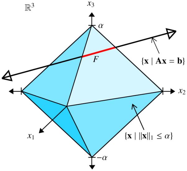
Nonunique intersection on ℓ₁-norm ball and line containing solutions, demonstrating potential failure of ℓ₁-norm based methods. The intersection is the set F, depicted by the red segment, which is contained in the nearest face of the ball.

In all the above cases, the most fundamental question we would like to be able to answer is whether an underdetermined system has a unique non-negative solution. That will be the first goal of this paper. If desired, we can then easily apply our results to other types of problems such as NNLS, Basis Pursuit, and LASSO via a mathematically-equivalent system as noted above.

2.1. Uniqueness conditions

To start, we will presume we have a compatible non-negatively-constrained system determined by A and b, arising either directly from our application, or, for example, from the NNLS or LASSO technique (from which we will henceforth replace b′ with b), and wish to investigate the uniqueness of the solutions in the set S _NN. By compatible here we mean at least one non-negative solution must exist. In [7] we investigated bounds for the solution set for non-negative systems by using linear programming to find the maximum and minimum of each element of the unknown. A similar technique was employed in [21] to test for uniqueness in LASSO. We can extend this idea to form conditions for uniqueness of x_k, the k^th element of x, over S _NN. First we test for uniqueness as follows,

$${\delta }_k=\begin{array}{c}\hfill \underset{\mathbf{x}\ge 0}{\text{max}}{x}_k\hfill \\ \hfill \mathbf{Ax}=\mathbf{b}\hfill \end{array}-\begin{array}{c}\hfill \underset{\mathbf{x}\ge 0}{\text{min}}{x}_k\hfill \\ \hfill \mathbf{Ax}=\mathbf{b}\hfill \end{array}=\begin{array}{c}\hfill \underset{\mathbf{x}\ge 0}{\text{max}}\left(x_k-x_k^{\prime }\right)\hfill \\ \hfill \mathbf{Ax}=\mathbf{b}\hfill \\ \hfill {\mathbf{Ax}}^{\prime }=\mathbf{b}.\hfill \end{array}$$ (4)

To find an upper bound on δ_k, we use duality theory for linear programs [6]. The dual of Eq. (4) is the linear program,

$$\begin{array}{cc}\hfill {\tilde{\delta }}_k=& \underset{\mathbf{y},{\mathbf{y}}^{\prime }}{\text{min}}{\mathbf{b}}^T(\mathbf{y}-{\mathbf{y}}^{\prime })\hfill \\ \hfill & {\mathbf{A}}^T\mathbf{y}\ge {\mathbf{e}}_k\hfill \\ \hfill & {\mathbf{A}}^T{\mathbf{y}}^{\prime }\le {\mathbf{e}}_k,\hfill \end{array}$$ (5)

where e_k is a vector of zeros except a one in the k^th element. For intuition, consider what we get without non-negativity constraints, where the possible solutions are the affine set {x | Ax = b}. It is straightforward to show that x_k takes on a unique value if and only if there is a solution $\widehat{\mathbf{y}}$ to ${\mathbf{A}}^T\widehat{\mathbf{y}}={\mathbf{e}}_k$. If we write these conditions as ${\widehat{\mathbf{y}}}_{\left(k\right)}^T\mathbf{A}={\mathbf{e}}_k^T$ for k = 1, …, n, and combine them into a matrix system, we fuind that these versions of the dual variables $\widehat{\mathbf{y}}$ are simply columns of the left inverse ${\widehat{\mathbf{Y}}}^T\mathbf{A}=\mathbf{I}$, where I is the identity matrix. If we similarly combine the n dual optimization problems of Eq. (5), we get the following combined problem for all elements (note that inequalities operate element-wise for matrices throughout this paper),

$$\begin{array}{c}\hfill \alpha =\underset{\mathbf{Y},{\mathbf{Y}}^{\prime },\mathbf{d}}{\text{min}}\parallel \mathbf{d}\parallel \hfill \\ \hfill {(\mathbf{Y}-{\mathbf{Y}}^{\prime })}^T\mathbf{b}=\mathbf{d}\hfill \\ \hfill {\mathbf{Y}}^T\mathbf{A}\ge \mathbf{I}\hfill \\ \hfill {\mathbf{Y}}^{\prime T}\mathbf{A}\le \mathbf{I},\hfill \end{array}$$ (6)

where ∥·∥ can be any norm. This vector d has elements which are the lengths of sides of the smallest box containing S _NN, the set of non-negative solutions. Its magnitude (∥d∥, the “distance from uniqueness”) gives us a metric for how tightly the system restricts the possible values of the unknown. Its length is the worst-case distance between any two members of the solution set.

Theorem 1

The compatible system Ax = b has a unique non-negative solution if and only if d = 0.

Proof. If d = 0, then all ${\tilde{\delta }}_k$ are zero. As ${\tilde{\delta }}_k$ are upper bounds for δ_k, each x_k can only take on a unique scalar value and hence x is unique. For the reverse direction, since we assume the system is compatible, Eq. (4) has an optimal solution. Further note that the optimal d will be the same regardless of norm, hence we can presume an ℓ₁-norm is used and use the strong duality conditions for linear programs to require that ${\tilde{\delta }}_k$ = δ_k. If x is unique then we must have δ_k = 0 for all k, and by strong duality this means ${\tilde{\delta }}_k$ = 0 for all k, i.e. d = 0.

2.2. Algorithm

Next we assume we are given a system which does not have a unique solution, and our goal is to find a “nearby” system for which d = 0, by adjusting b. Specifically we desire a residual Δb such that (Y − Y′)^T (b + Δb) = 0 in Eq. (6). However, a variable Δb here produces a nonconvex quadratic constraint, as we will have products between Δb and both Y and Y′. We will address this with an iterative algorithm based on successive linear approximations of this constraint. Given a tolerance μ, we solve the following algorithm for successive updates to b:

STEP 1. Solve Eq. (6) for d^∗, Y^∗ and Y′^∗.

STEP 2. If ∥d∥≤ μ, stop, otherwise choose ϵ where 0 ≤ ϵ < ∥d∥, and solve Eq. (7) for Δb and x using the d^∗, Y^∗ and Y′^∗ computed in STEP 1.

$$\begin{array}{c}\hfill \beta =\underset{\mathbf{x}\ge 0,{\Delta }_b}{\text{min}}\parallel \Delta \mathbf{b}\parallel \hfill \\ \hfill \parallel {({\mathbf{Y}}^{\ast }-{\mathbf{Y}}^{\prime \ast })}^T\Delta \mathbf{b}+{\mathbf{d}}^{\ast }\parallel \le ϵ\hfill \\ \hfill \mathbf{Ax}=\mathbf{b}+\Delta \mathbf{b}\hfill \end{array}$$ (7)

The constraints here are linear, so the problem is convex. Note that Eq. (7) can be viewed as a NNLS problem (compare to Eq. (1)) with an added constraint to impose uniqueness .

STEP 3. Update b by accumulating new residual adjustment from STEP 2 (i.e., b = b + Δb) and goto STEP 1.

The following theorem proves that a solution found via the above algorithm produces a system with a unique solution following an iteration where we picked ϵ = 0, which we may choose to do in a single iteration or after multiple iterations (the only difference will be how globally-optimal the resulting Δb might be). In practice we should use a small positive value instead of zero for E, due to numerical precision issues.

Lemma 1

The optimal x^∗ found by Eq. (7) with ϵ = 0, using the d^∗, Y^∗ and Y′^∗ computed in Eq. (6), will be the unique non-negative solution in the new system modified by the optimal Δb^∗, i.e., {x^∗} = {x | Ax = b + Δb^∗, x ≥ 0}.

Proof. This holds for any feasible point for the problem of Eq. (7), the optimal is simply a choice with minimal residual. Given a feasible point $(\widehat{\mathbf{x}},\Delta \widehat{\mathbf{b}})$, $\widehat{\mathbf{x}}$ is a solution in the set $\{\mathbf{x}\mid \mathbf{Ax}=\mathbf{b}+\Delta \widehat{\mathbf{b}},\mathbf{x}\ge 0\}$, which means the system is compatible. Further, $\Delta \widehat{\mathbf{b}}$ solves the system ${({\mathbf{Y}}^{\ast }-{\mathbf{Y}}^{\prime \ast })}^T\Delta \widehat{\mathbf{b}}=-{\mathbf{d}}^{\ast }$. By combining the constraints from Eq. (6) with our equation for $\Delta \widehat{\mathbf{b}}$, we have

$$\begin{array}{c}\hfill {({\mathbf{Y}}^{\ast }-{\mathbf{Y}}^{\prime \ast })}^T(\mathbf{b}+\Delta \widehat{\mathbf{b}})=0\hfill \\ \hfill {\mathbf{Y}}^{\ast T}\mathbf{A}\ge \mathbf{I}\hfill \\ \hfill {\mathbf{Y}}^{\prime \ast T}\mathbf{A}\le \mathbf{I}.\hfill \end{array}$$ (8)

These equations are the constraints of Eq. (6) with b replaced by $\mathbf{b}+\Delta \widehat{\mathbf{b}}$. This means we can perform the optimization problem of Eq. (6) with b also replaced by $\mathbf{b}+\Delta \widehat{\mathbf{b}}$ and get the minimizer d = 0. By Theorem 1, this means the non-negative solution to Ax = $\mathbf{b}+\Delta \widehat{\mathbf{b}}$ must be unique.

It can further be shown that it is possible to achieve any desired tolerance μ on the size of the solution set by choosing ϵ = μ, using the fact that μ = ∥d_(final)∥ = ∥(Y^∗ − Y′^∗)^T (b + Δb)∥ = ∥(Y^∗ − Y′^∗)^T Δ$\widehat{\mathbf{x}}$ + d^∗∥ ≤ ϵ. Finally we argue that the closer we make ϵ to ∥d^∗∥ in each iteration, the more accurately our linearized constraint fits the true constraint at each iteration, as it is quadratic. This is not necessary for Theorem 1, which only deals with feasible points, but in practice it suggests we can achieve a smaller net lΔb∥ by performing more iterations. We will demonstrate the performance of single versus multiple iteration settings in the next section.

3. Simulations

We performed a variety of numerical simulations to demonstrate the technique. For each simulation, given a particular n and m, we formed a matrix using a choice of model to generate elements. For most cases we generated a true x with K nonzero values at uniformly-random locations, and generated each of those K values using a uniform distribution over the interval [0, 1] (unless stated otherwise). We added Gaussian noise to the resulting measurement vector b to achieve an SNR of 10:1. We then performed a denoising step using NNLS to make a compatible system as a starting point. Finally we estimated d for the system, if it was unbounded (meaning our system did not fulfill the positive orthant condition), or if it was very small (meaning our system essentially had a unique non-negative solution already), the system was discarded and a new one was randomly generated with the same parameters. For the algorithm we used a tolerance of μ = 0.01.

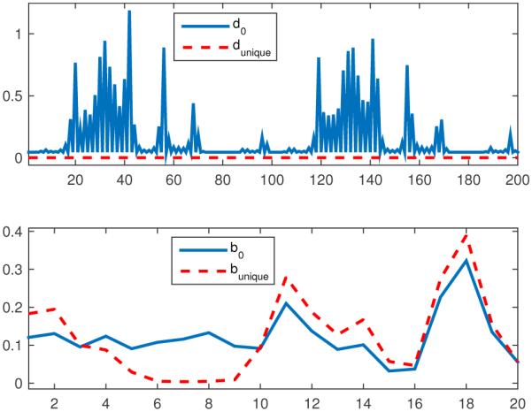
For example, Fig. 2 gives the true solution and the unique solution estimated via our technique for a matrix generated using uniformly-distributed random elements with values in [0, 1], with n = 100, m = 30, and K = 15. For this example we used ϵ = 0.01, requiring only a single iteration to achieve the final tolerance. Fig. 2 also gives the non-negative ℓ₁ (min ℓ₁-norm over non-negative x). In Fig. 3 we give d for the initial system as (denoted as d₀), which gives the range each element of the solution could initially take. After running our algorithm we computed d again (d_unique), measuring the range taken by each element of {x | Ax = b + Δb, x ≥ 0}. As we can see from Fig. 3, d_unique is essentially zero meaning our system now admits a unique solution. Fig. 3 also gives the corresponding initial (b₀) and adjusted (b₀ + Δb = b_unique) versions of b. We can see that b₀ required only a very-small adjustment to form b_unique in this case. Figs. 4 and 5 provide similar results for a non-bounded example for which the minimum ℓ₁ solution was not unique, using a model that performs a low-pass filtering operation. The system was converted to a non-negative system in 2n dimensions, then the algorithm was applied to enforce a unique solution, and finally the resulting system was converted back to n dimensions, yielding a system with a unique minimum ℓ₁ norm.

Figure 2.

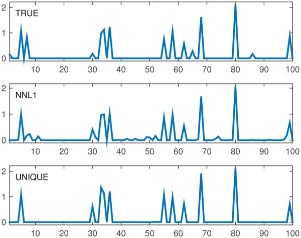
True, Non-negative-ℓ₁ (NNL1), and unique solutions for uniform random matrix example, n = 100, m = 30, K = 15 = ∥x_true∥₀.

Figure 3.

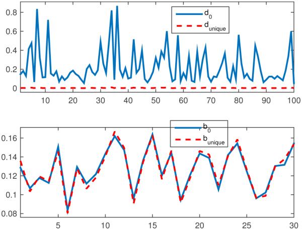
Displacement (d) from uniqueness for original and unique system, and output vector (b) for original and unique system.

Figure 4.

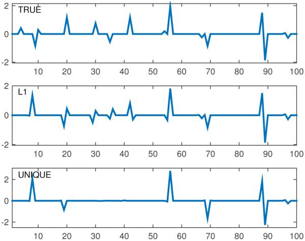
True, minimum ℓ₁ (L1), and unique solutions for non-bounded example, n = 100, m = 30, K = 15.

Figure 5.

Displacement (d) from uniqueness for original and unique system, and output vector (b) for original and unique system. Non-bounded example.

We investigated the algorithm’s performance by generating 100 realizations using models with uniform random elements (Fig. 6) and binary random elements (Fig. 7), where for each realization we used a new random A, new true x (changing both the values and locations), and new noise. We compared the cardinality of the result computed with our algorithm both with single-iteration settings, and with a multiple-iteration approach where ϵ was chosen to be 90 percent of the maximum element of d computed in each previous iteration. For the single-iteration unique solutions in Fig. 6, we find a clear trend towards sparser solutions as ∥d₀∥ (the initial distance from uniqueness) increases, while in Fig. 7 we see that only the multiple-iteration approach produced non-trivial results. We also computed the minimum non-negative ℓ₁ solutions using the same denoised starting point as the proposed algorithm, and plotted the cardinalities of all of these solutions versus ∥d₀∥. We see that for the uniform system, we found comparable performance with both the proposed multiple-iteration algorithm and the NNL1 solution, while for the binary system, the proposed algorithm demonstrated superior performance, consistently returning a sparse solution.

Figure 6.

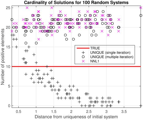
Number of positive elements (x_i ≥ 0.02) for true, Non-negative ℓ₁ denoised (NNL1), and unique solutions for 100 different noisy realizations of uniform model, SNR = 10, n = 100, m = 25, K = 10 = ∥x_true∥₀.

Figure 7.

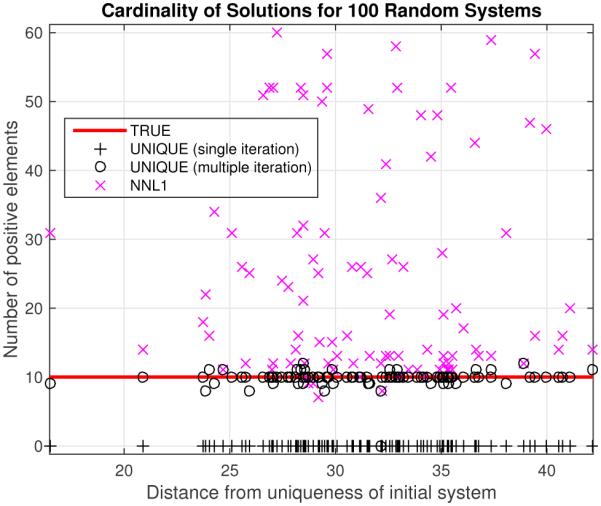
Number of positive elements (x_i ≥ 0.02) for true, Non-negative ℓ₁ denoised (NNL1), and unique solutions for 100 different noisy realizations of convolution model, SNR = 10, n = 100, m = 11, K = 10 = ∥x_true∥₀. In this case, the NNL1 technique often failed to yield a sparse solution while the proposed technique consistently succeeded using the multiple-iteration algorithm.

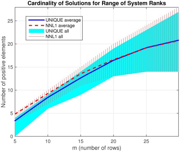
Next we repeated similar 100-realization simulations for a range of different model sizes using matrices formed by three different random distributions. The results are summarized in Figs. 8, 9, and 10, where the range of resulting cardinalities achieved at each m is shown by the solid regions. For each model we varied m between a minimum of 5 and a maximum of the highest that was reasonably possible to still find non-unique systems (systems for which the solution was not already unique without adjustment) with that approach, generally around 25 to 30. At around m = 5 we see that the proposed algorithm began to return all-zero results as the single-iteration case did, suggesting that a more sophisticated linearization is needed (e.g., more iterations). At higher values of m, we see comparable results for the proposed and NNL1 algorithms for the uniform and gaussian models, generally achieving a cardinality comparable to m. For the binary model, we see that the NNL1 algorithm consistently returns many non-sparse results as seen in Fig. 7. In Fig. 11 we give the average (Pearson) correlation for each m for the methods between the estimate and the true solution. For the uniform and Gaussian models we see that the proposed algorithm generally achieved a slightly higher correlation with the true solution for smaller values of m, presumably due to the bias of the ℓ₁ estimate. At higher m the NNL1 correlation was slightly higher, probably due to the 0.01 gap the proposed algorithm allows in uniqueness for numerical reasons. For the binary model, the NNL1 achieved a higher correlation, but recall this was the case where NNL1 often return dense solutions. To make a fairer comparison, we imposed ℓ₁ regularization via LASSO to achieve a comparable sparsity for the failure cases (the regularization parameter was increased until a solution with cardinality of at most m was achieved), which led to a lower correlation overall.

Figure 8.

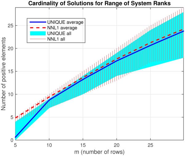
Range of cardinality of solutions for Non-negative ℓ₁ denoised (NNL1), and unique solutions using ϵ = 0.9 max(d), for 100 different noisy realizations of uniform random system, for each value of m ranging in steps of 5 between 5 and 30 (600 total realizations), SNR = 10, n = 100, K = 10 = ∥x_true∥₀.

Figure 9.

Range of cardinality of solutions for Non-negative ℓ₁ denoised (NNL1), and unique solutions using ϵ = 0.9 max(d), for 100 different noisy realizations of Gaussian random system, again for each m between 5 and 30, SNR = 10, n = 100, K = 10 = ∥x_true∥₀.

Figure 10.

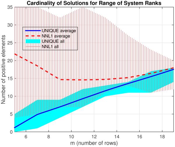
Range of cardinality of solutions for Non-negative ℓ₁ denoised (NNL1), and unique solutions using ϵ = 0.9 max(d), for 100 different noisy realizations of binary random system for each m between 5 and 20, SNR = 10, n = 50, K = 10 = ∥x_true∥₀. Again we see the failure to achieve a sparse solution for many cases with the NNL1 technique.

Figure 11.

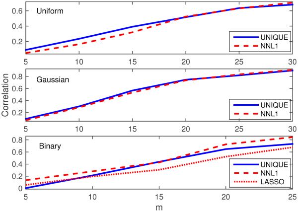
Average Pearson correlation between estimates and true solutions for each m for the simulations of Figs. 8, 9, and 10. Since the NNL1 solutions often failed to be sparse for the Binary model, and hence the correlation may demonstrate over-fitting, a non-negative LASSO estimate was calculated using increased regularization to achieve comparable sparsity to the UNIQUE solution.

Finally we compared the proposed approach to a LASSO-based technique in achieving a system with a unique solution. We compared the proposed algorithm with a non-negative LASSO algorithm, wherein we increased the regularization parameter λ until the adjusted system {x | Ax = b + Δb_LASSO, x ≥ 0} has a unique solution (the smallest λ where d is below our threshold of 0.01). Note that this is stricter than a requirement that only the set of LASSO minimizers be unique. In Fig. 12 we give the cardinality and fractional residual (computed as ∥Δb∥/∥b∥) for each of the 100 realizations. We see that generally the LASSO approach used a much larger adjustment to the system to achieve a unique system solution, and for many cases was unable to produce a non-trivial unique solution.

Figure 12.

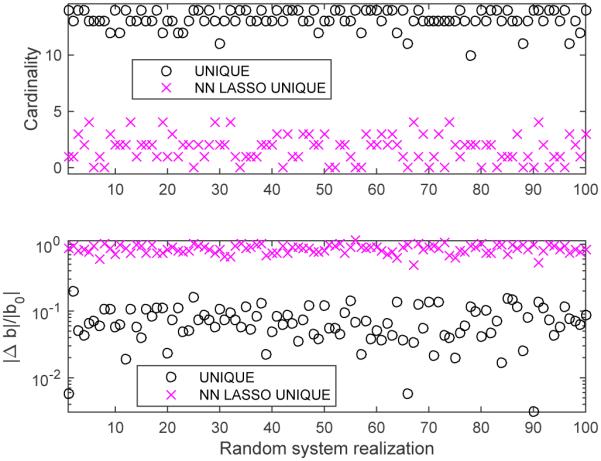
Cardinality and fractional change in Δb for unique solutions using proposed algorithm versus LASSO with ϵ = 0.9 max(d), for 100 different noisy realizations of uniform random system, for SNR = 10, m = 15, n = 100, K = 10 = ∥x_true∥₀. We see that the proposed algorithm generally achieved a sparse solution with cardinality comparable to m, and with a change in b comparable to the SNR. Attempting to manufacture a system that has a unique solution using LASSO was far less successful, yielding results that were overly-sparse with an excessively-large fractional change in b.

4. Discussion

In this paper we derived uniqueness conditions for the non-negative solution to an underdetermined linear system using optimization theory. The conditions provide a kind of distance from uniqueness for when the system is non-unique, which we used in an algorithm to adjust the system and make a similar system which has a unique solution. We provided simulated examples to demonstrate the qualitative behavior of the technique where we demonstrated a broad ability to find non-trivial unique solutions over a range of systems. For systems with elements drawn from a continuous distribution, performance appears comparable to ℓ₁-based methods, while for more structured systems such as the binary model, the performance of the proposed algorithm appears to be superior, presumably due to difficulties in achieving a unique optimal with the ℓ₁-norm in such cases. The question of reconstruction error is beyond the scope of this paper as we do not make assumptions about matrix properties beyond the positive orthant condition, but the correlations in the simulations proved comparable to and often better than achieved with ℓ₁-based techniques, suggesting this would be a fruitful area for further research.

Multiple improvements or variations are possible with this algorithm. A more intelligent choice of iteration settings would likely address the failure cases, such as with small m. More generally, note that Lemma 1 applies to any feasible point, meaning we can choose an optimal however we wish. We chose the minimum residual on Δb defined using the ℓ₂-norm, but we might employ a different norm such as the ℓ₁-norm, for example, to get a sparse residual. We might also impose other desired properties such as additional solution sparsity via a ℓ₁-norm regularization term on the unique solution itself, yielding a hybrid approach. We might also utilize other means to convert a general linear system into a non-negative one which satisfies the positive orthant condition, for example by augmenting the matrix with an additional row that is optimized somehow for the particular scenario. Finally, it would be straightforward to replace the non-negativity constraint with other constraints, such as a conic constraint or other convex inequalities.

The approach of finding the nearest unique solution is interesting from multiple perspectives. First is simply its ability to indirectly provide a sparse solution, as sparsity is the basis for uniqueness in a non-negative system and the related ℓ₁-norm based techniques. But another interesting perspective is the idea of uniqueness itself as a form of prior knowledge or model design requirement. If our goal is to choose Δb to minimize the uncertainty in x, then a choice for which x must be unique is the best possible in a sense. The unique solution might also be utilized as a component of the solution set, as in dimensionality reduction, rather than a model in itself.

References

- [1].Bruckstein AM, Elad M, Zibulevsky M. On the uniqueness of non-negative sparse & redundant representations. IEEE International Conference on Acoustics, Speech and Signal Processing, 2008. ICASSP 2008; IEEE; Mar, 2008. pp. 5145–5148. [Google Scholar]
- [2].Bruckstein AM, Elad M, Zibulevsky M. On the Uniqueness of Nonnegative Sparse Solutions to Underdetermined Systems of Equations. IEEE Transactions on Information Theory. 2008 Nov;54(11):4813–4820. [Google Scholar]
- [3].Bruckstein AM, Elad M, Zibulevsky M. Sparse non-negative solution of a linear system of equations is unique. 3rd International Symposium on Communications, Control and Signal Processing, 2008. ISCCSP 2008; IEEE; Mar, 2008. pp. 762–767. [Google Scholar]
- [4].Candes Emmanuel J. The restricted isometry property and its implications for compressed sensing. Comptes Rendus Mathematique. 2008 May;346(9¢10):589–592. [Google Scholar]
- [5].Chen Scott Shaobing, Donoho David L., Saunders Michael A. Atomic Decomposition by Basis Pursuit. SIAM Review. 2001 Jan;43(1):129–159. [Google Scholar]
- [6].Dantzig George. Linear Programming and Extensions. Princeton University Press; Aug, 1998. [Google Scholar]
- [7].Dillon Keith, Fainman Yeshaiahu. Bounding pixels in computational imaging. Applied Optics. 2013 Apr;52(10):D55–D63. doi: 10.1364/AO.52.000D55. [DOI] [PubMed] [Google Scholar]
- [8].Donoho David L., Elad Michael. Optimally sparse representation in general (nonorthogonal) dictionaries via ¢1 minimization. Proceedings of the National Academy of Sciences. 2003 Mar;100(5):2197–2202. doi: 10.1073/pnas.0437847100. [DOI] [PMC free article] [PubMed] [Google Scholar]
- [9].Donoho David L., Tanner Jared. Neighborliness of randomly projected simplices in high dimensions. Proceedings of the National Academy of Sciences of the United States of America. 2005 Jul;102(27):9452–9457. doi: 10.1073/pnas.0502258102. [DOI] [PMC free article] [PubMed] [Google Scholar]
- [10].Donoho David L., Tanner Jared. Sparse nonnegative solution of underdetermined linear equations by linear programming. Proceedings of the National Academy of Sciences of the United States of America. 2005 Jul;102(27):9446–9451. doi: 10.1073/pnas.0502269102. [DOI] [PMC free article] [PubMed] [Google Scholar]
- [11].Kay Steven M. Fundamentals of Statistical Signal Processing: Estimation Theory. Prentice-Hall PTR; 1998. [Google Scholar]
- [12].Khajehnejad MA, Dimakis AG, Xu Weiyu, Hassibi B. Sparse Recovery of Nonnegative Signals With Minimal Expansion. IEEE Transactions on Signal Processing. 2011 Jan;59(1):196–208. [Google Scholar]
- [13].Kotz Samuel, Kozubowski Tomasz, Podgorski Krzysztof. The Laplace Distribution and Generalizations: A Revisit With Applications to Communications, Exonomics, Engineering, and Finance. Springer; Jun, 2001. [Google Scholar]
- [14].Lawson C, Hanson R. Solving Least Squares Problems. Society for Industrial and Applied Mathematics; Jan, 1995. Classics in Applied Mathematics. [Google Scholar]
- [15].Lin Tsung-han, Kung HT. Stable and Efficient Representation Learning with Nonnegativity Constraints. 2014:1323–1331. [Google Scholar]
- [16].Osborne Michael R., Presnell Brett, Turlach Berwin A. On the LASSO and its Dual. Journal of Computational and Graphical Statistics. 2000 Jun;9(2):319–337. [Google Scholar]
- [17].Slawski Martin, Hein Matthias. Sparse recovery by thresholded non-negative least squares. In: Shawe-Taylor J, Zemel RS, Bartlett PL, Pereira F, Weinberger KQ, editors. Advances in Neural Information Processing Systems 24. Curran Associates, Inc.; 2011. pp. 1926–1934. [Google Scholar]
- [18].Slawski Martin, Hein Matthias. Non-negative least squares for high-dimensional linear models: Consistency and sparse recovery without regularization. Electronic Journal of Statistics. 2013;7:3004–3056. [Google Scholar]
- [19].Slawski Martin, Hein Matthias, Campus E. Sparse recovery for protein mass spectrometry data. Practical Applications of Sparse Modeling. 2014:79. [Google Scholar]
- [20].Tibshirani Robert. Regression Shrinkage and Selection Via the Lasso. Journal of the Royal Statistical Society, Series B. 1994;58:267–288. [Google Scholar]
- [21].Tibshirani Ryan J. The lasso problem and uniqueness. Electronic Journal of Statistics. 2013;7:1456–1490. [Google Scholar]
- [22].Wang Meng, Tang Ao. Conditions for a unique non-negative solution to an underdetermined system. 47th Annual Allerton Conference on Communication, Control, and Computing, 2009. Allerton 2009; IEEE; Sep, 2009. pp. 301–307. [Google Scholar]
- [23].Wang Meng, Xu Weiyu, Tang Ao. A Unique ¢ÅNonnegative¢ Solution to an Underdetermined System: From Vectors to Matrices. IEEE Transactions on Signal Processing. 2011 Mar;59(3):1007–1016. [Google Scholar]
- [24].Willett Rebecca M., Marcia Roummel F., Nichols Jonathan M. Compressed sensing for practical optical imaging systems: a tutorial. Optical Engineering. 2011;50(7):072601–072601–13. [Google Scholar]
- [25].Ziegler Günter M. Lectures on Polytopes. Springer; 1995. [Google Scholar]