False discovery rates for rare variants from sequenced data

Abstract

The detection of rare deleterious variants is the pre-eminent current technical challenge in statistical genetics. Sorting the deleterious from neutral variants at a disease locus is challenging because of the sparseness of the evidence for each individual variant. Hierarchical modeling and Bayesian model uncertainty are two techniques that have been shown to be promising in pinpointing individual rare variants that may be driving the association. Interpreting the results from these techniques from the perspective of multiple testing is a challenge and the goal of this article is to better understand their false discovery properties. Using simulations, we conclude that accurate false discovery control cannot be achieved in this framework unless the magnitude of the variants’ risk is large and the hierarchical characteristics have high accuracy in distinguishing deleterious from neutral variants.

1 Introduction

The predominant contemporary issue in the field of statistical genetics in cancer is how to identify and characterize the effects of rare variants that influence disease risk. New next generation sequencing (NGS) techniques are rapidly being developed and will gradually become the technology of choice in the next few years. The challenge will lie in using the vast quantities of data generated by NGS to try to sort harmful from harmless variants at a risk locus in order to properly counsel individuals who learn from genetic testing that they have a mutation in an important cancer gene. Identification of rare deleterious variants in this setting is a formidable statistical challenge since these are observed very infrequently and these sparse frequencies on their own are insufficient to provide meaningful risk predictions. In earlier work we developed a hierarchical modeling approach for case-control studies in which multiple rare variants at a known risk locus are examined individually (Capanu et al. 2008; Capanu and Begg 2011). The essential lever for accomplishing this is the presence of hierarchical covariates that are associated with disease risk and that can be used for implicitly aggregating the rare variants to permit stronger inferences about individual variants. These hierarchical covariates are characteristics of the variants themselves, such as the degree of conservation across species, the position on the gene, and other features that can be represented using bioinformatic measures (Ng and Henikoff 2001, 2002; Sunyaev et al. 2000, 2001; Ramensky et al. 2002; Tavtigian et al. 2006). Quintana et al. (2012) also advocated the use of external biological knowledge about the variants to help boost the power of detecting truly causal variants and proposed an integrative Bayesian model uncertainty (iBMU) method to achieve this.

In a previous study of rare missense variants in the BRCA1 and BRCA2 genes using data from a large case-control study of contralateral breast cancer our hierarchical modeling approach indicated that 6 of the 181 rare variants analyzed had nominally statistically significant associations with risk at the 0.05 significance level (Capanu et al. 2011). An important issue to recognize when reporting large numbers of statistical tests is the fact that many of the tests will have false positive findings and that interpretation of the validity of any “discoveries” must recognize the likely extent of false discovery.

To handle multiple testing problems, Benjamini and Hochberg (1995) introduced the false discovery rate (FDR) as the expected proportion of false positive findings among all the statistically significant associations. The FDR approach has become very popular due to its power advantage over conventional Bonferroni type corrections. That is, it detects more true positive associations. To further improve power, multiple modifications to the original FDR approach have been proposed (Genovese and Wasserman 2002; Storey 2002; Genovese et al. 2006; Benjamini et al. 2006; Yekutieli 2008; Zeisel et al. 2011, among others). An assumption behind the traditional FDR procedure is that the tests performed are statistically independent. However in our context the model involves an implicit sorting of the variants based on hierarchical covariates, followed by the estimation of relative risks and confidence intervals for each of possibly several hundred or even thousands of individual rare variants within the locus. Consequently, the estimates and tests for individual variants may be correlated, due to their dependence on the higher level covariates.

Numerous investigators have examined the impact of correlations between tests on the properties of the FDR and related statistics. Some have proposed resampling procedures to control the FDR in the presence of correlation (Yekutieli and Benjamini 1999; Storey and Tibshirani 2001; Storey 2002; Romano et al. 2008), while others have introduced step-up (Blanchard and Roquain 2008; Sarkar 2008), step-down (Ge et al. 2008), adaptive (Benjamini et al. 2006; Blanchard and Roquain 2009), or more general procedures (Li and Ji 2005; Efron 2004, 2007a; Storey 2007; Efron 2010). Some authors have shown that under specific situations, a certain degree of dependency is allowed among the test statistics with no need for any modification of the standard FDR corrections (Li et al. 2005; Farcomeni 2007; Clarke and Hall 2009).

It is not clear whether the preceding methods can be applied to address the multiplicity arising in testing rare variants in the context of hierarchical models. Indeed Gelman et al. (2009) have even questioned the need for multiple testing when employing hierarchical models, arguing that multilevel models address the multiple testing problem through the phenomenon of “shrinkage”. In our analyses we have certainly observed a lot of shrinkage of the risk estimates for the individual rare variants (Capanu et al. 2008, 2011) with many variants estimated to have a relative risk close to 1 while risk estimates are well above 1 for a select group of potentially deleterious variants. Note that under the Bayesian model uncertainty framework of Quintana and Conti (2013) the prior inclusion probability of each rare variant in the analysis can range from a uniform prior across the model space to a more structured prior that maintains a constant global prior probability (prior probability that at least one of the variants is associated) regardless of how many variants are included in the analysis. The latter choice provides an implicit multiplicity correction as it assures that the global prior probability of an association will not increase as the number of variants in an analysis increases (Wilson et al. 2010).

Each variant is of crucial interest to the individuals and their family members who possess the specific variant, and thus accurate classification of all variants as deleterious versus neutral is a pivotal goal. A significant step towards achieving this goal is to identify candidate variants that are potentially deleterious that would then require further validation. For this purpose, it is important to recognize how many of the variants deemed deleterious by our hierarchical model are in fact neutral, and what proportion of variants deemed neutral by the method are in fact deleterious. In this article we study the false discovery properties of several available techniques when testing large numbers of rare variants in the context of a hierarchical model.

2 Motivating Example

The motivating study for this research, the Women’s Environmental, Cancer, and Radiation Epidemiology, [WECARE] Study (Bernstein et al. 2004) is a case-control study that involved 705 cases, women with asynchronous contralateral breast cancer (CBC), and 1398 controls with unilateral breast cancer. Screening for BRCA1 and BRCA2 mutations identified 470 unique sequence variants, of which 181 were rare missense variants (with MAF <= 2.5%). Of the 181 rare missense variants, 115 variants (64%) were carried by only one subject, 29 were carried by 2 subjects, 11 were carried by 3 subjects, 6 were carried by 4 participants, 7 were carried by 5 to 9 subjects, and 14 were carried by 10 or more subjects (see Borg et al. 2010, for more details).

We applied the hierarchical modeling approach to the WECARE BRCA1 /BRCA2 data (Capanu et al. 2011) and the results showed that the vast majority of the rare missense variants investigated are neutral, but supported the growing evidence that there exists a small subgroup of missense variants that are deleterious. Specifically, the analysis concluded that of the 181 rare missense variants examined in the model, 6 emerged as having nominally statistically significant association with risk (at the conventional 0.05 level). In practice we expect 1 statistically significant result for every 20 independent tests performed, and so at first glance the identification of 6 significant results from the 181 variants seems unremarkable. However, interpreting our results from the perspective of multiple testing is challenging in a setting where the information content (i.e. numbers of subjects with the variant) is very sparse, and in the context of a hierarchical model which implicitly aggregates the information from variants that share higher-order characteristics. Nonetheless, the histogram of estimated relative risks in Figure 1 appears to support empirically the hypothesis that there is a small subset of harmful variants as indicated by the small upper tail to the distribution.

Figure 1.

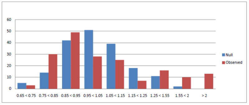
Hierarchical modeling estimates of relative risks for 181 rare missense variants (red histogram) versus expected distribution if no rare variants affect risk (blue histogram). Published as Figure 1 in Capanu et al. (2011)

Figure 2 shows the histogram of corresponding z-values from the WECARE BRCA1/BRCA2 analysis with the standard normal density superimposed. The plot indicates a departure of the z-values from N(0, 1), with the standard normal distribution being too wide for the data. This suggests that any multiple testing procedure employing the standard normal distribution as the reference distribution for computing p-values will result in conservative p-values. This histogram also suggests a mixture of distributions, i.e. deleterious and neutral, which led us to explore Efron’s local false discovery rate approach since this technique is based on such an assumption.

Figure 2.

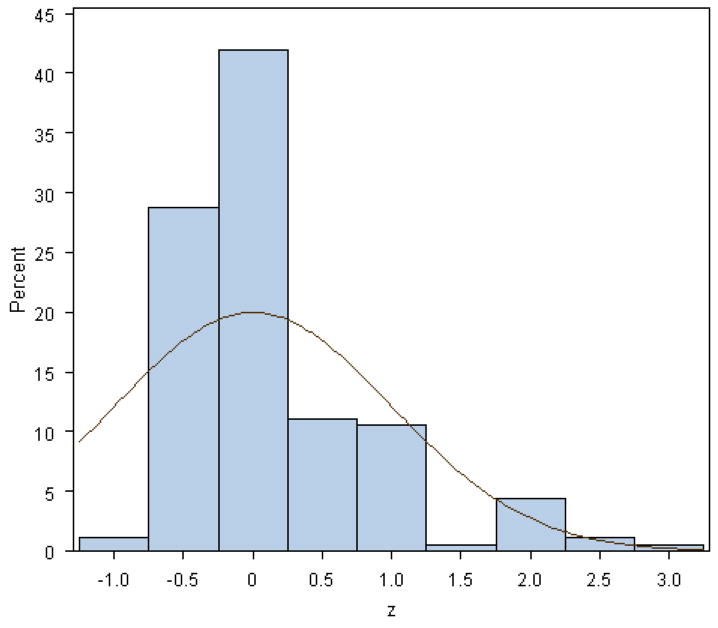
Histogram of the z-values obtained from the hierarchical modeling analysis of the WECARE BRCA data. Standard normal density is overimposed.

3 Methods

In this section, we briefly outline two techniques that can be used to prioritize individual rare variants and incorporate prior information - our hierarchical model approach and the integrative Bayesian model uncertainty method of Quintana and Conti (2013), we describe several available FDR controlling procedures, and conduct a simulation study to investigate the FDR properties of these methods in the context of our hierarchical model.

3.1 Hierarchical Model

The fundamental data configuration is a case-control study with N participants, with the case and control status of each participant denoted by the N×1 vector Y . In addition to a set of subject specific covariates representing risk factors, captured by the design matrix U and corresponding regression parameters λ, each participant is characterized by the presence or absence of each of a set of n genetic variants within the candidate gene under investigation. The constellation of combinations of these variants is contained in the design matrix X, and β represents an n × 1 vector of parameters of the log relative risks conferred by each of the variants.

The model combines a first stage logistic regression with a second stage linear regression. In the first stage, the outcome vector Y is related to β and λ through the model:

$$\mathrm{logit}P(Y|X,U)=X\beta +U\lambda .$$ (1)

In the second stage the individual log relative risks of the variants (β) are modeled as a function of biological features of the variant that may indicate the likely relevance of the variant to the functioning of the gene. For example in our analysis of the WECARE BRCA1/BRCA2 data we employed the bioinformatic tools SIFT (Ng and Henikoff 2001), PolyPhen (Sunyaev et al. 2000), and Grantham scores (Tavtigian et al. 2006)). The second stage model is thus defined by

$$\beta =Z\pi +\delta ,\mathrm{with}\delta \sim N(0,{\tau }^2{I}_n),$$ (2)

where the n × m matrix Z captures the hierarchical information about the variants (with Z_ij independent of Z_kj for i, k in 1, … , n, for any j in 1, … , m), π is an m × 1 column vector of the second stage parameters that capture the influences on the log relative risk of each of the hierarchical covariates and δ is a vector of normally distributed residual effects, assumed (for convenience) to be statistically independent. Here I_n denotes the n × n identity matrix.

By combining the first and second stage models we obtain a mixed effects logistic model:

$$\mathrm{logit}P(Y|X,U)=X(Z\pi +\delta )+U\lambda =XZ\pi +X\delta +U\lambda ,$$ (3)

which we estimate using a hybrid method that involves pseudo-likelihood estimation of the relative risk parameters with Bayesian estimation of the variance components, a strategy that exhibited superior performance compared to competitor estimation techniques studied in this setting (Capanu and Begg 2011).

3.2 Integrative Bayesian model uncertainty

Similar to the hierarchical modeling approach described in Section 3.1, we assume that the data consists of the N ×1 vector Y , an N × n matrix X composed of the measured predictors to be included in the model search, and an N × q matrix U of patient level confounders. The Bayesian model uncertainty (BMU) framework (Clyde and George 2004; Hoeting et al. 1999; Quintana et al. 2011) specifies each model M_γ ∈ M by an n dimensional indicator vector γ where γ_j = 1 if the predictor variable X_j is included in the model M_γ and γ_j = 0 if X_j is not included in model M_γ. Each model M_γ ∈ M is thus defined by a unique subset of the n predictor variables of interest.

In our setting of case-control association studies, the model M_γ relating the case-control status Y to the subset of predictor variables X_γ is a logistic regression

$$M_{\mathrm{\gamma }}:\mathit{logit}(Y=1)={\lambda }_0+U\lambda +X_{\mathrm{\gamma }}{\beta }_{\mathrm{\gamma }},$$

where λ₀ is the intercept common to every model, λ is the coefficient vector of confounders variables, X_γ is some parametrization of the set of predictors included in model M_γ and β_γ is the model-specific effect of X_γ on the case-control status. In our setting of rare variants, X_γ can be defined as the risk index of the rare variants included in M_γ as described by Quintana et al. (2011).

Following Quintana et al. (2011), the posterior model probabilities are defined as

$$p(M_{\mathrm{\gamma }}|Y)=\frac{p(Y|M_{\mathrm{\gamma }})p(M_{\mathrm{\gamma }})}{{\mathrm{\sum }}_{M_{\mathrm{\gamma }}\in M}p(Y|M_{\mathrm{\gamma }})p(M_{\mathrm{\gamma }})},$$

the posterior inclusion probabilities are computed as

$$p({\mathrm{\gamma }}_j|Y)=\sum _{M_{\mathrm{\gamma }}\in M:{\mathrm{\gamma }}_j=1}p(M_{\mathrm{\gamma }}|Y),$$

and the marginal Bayes factors (MargBF) are defined as the posterior odds divided by the prior odds for inclusion

$$BF[{\mathrm{\gamma }}_j=1:{\mathrm{\gamma }}_j=0]=\frac{p({\mathrm{\gamma }}_j=1|Y)}{p({\mathrm{\gamma }}_j=0|Y)}/\frac{p({\mathrm{\gamma }}_j=1)}{p({\mathrm{\gamma }}_j=0)}.$$

Quintana and Conti (2013) extended the BMU framework outlined above to incorporate information characterizing the predictors and Quintana et al. (2012) applied it to the setting of rare variants to inform the selection of associated variants. They achieve this by introducing a second-stage regression that includes p variant-level covariates contained in an n×p matrix W quantifying external information on the relationships between the n variants. They use a probit model linking the p variant-level covariates corresponding to variants X_j to the probability that each variant is associated by introducing a latent vector t. Each element of t is assumed normally distributed

$$t_j|\alpha \sim N({\alpha }_0+W_j^{\prime }\alpha ,1).$$

Then the inclusion indicator for X_j into model M_γ is obtained as γ_j = I[t_j > 0]. The parameter α₀ is set to be α₀ = Φ⁻¹(2^−1/p) on the basis of the multiplicity corrected model space priors introduced in Wilson et al. (2010) to insure that the global prior probability is maintained constant, this way providing an intrinsic multiplicity correction. The second-stage model specification is completed by assuming that the prior distribution of α is α ~ N(0, I_p).

By iterating between a Metropolis-Hastings and a Gibbs sampling algorithm they approximate the posterior probability of each model and obtain the posterior quantities needed for formal inference, the marginal posterior inclusion probabilities and the MargBF. More details on these derivations and the iBMU approach can be found in Quintana et al. (2012); Quintana and Conti (2013).

In our simulations and analysis we implemented the iBMU approach using the functions from the BVS R package (Quintana 2012) based on 100000 iterations and with the “regions” option to distinguish between BRCA1 and BRCA2; all other options were left at their default settings.

3.3 Benjamini-Hochberg false discovery controlling procedure

Modern multiple testing algorithms are based on control of the FDR introduced by Benjamini and Hochberg (1995) as the expected proportion of false positive findings among all the statistically significant associations. Specifically, suppose we are testing H₁, H₂, … , H_n hypotheses (which in our setting correspond to H₀ : β₁ = … = β_n = 0) based on the corresponding p-values p₁, p₂, … , p_n. If p₍₁₎, p₍₂₎, … , p_(n) denote the p-values ordered from the smallest to the largest and H_(i) is the null hypothesis corresponding to p_(i), then the multiple testing procedure proposed by Benjamini and Hochberg is defined as follows: reject all hypotheses H_(i), i = 1, … , k, where k is the largest i for which $p_{(i)}\le \frac{i}{n}\alpha .$. This sequential p-value method ensures control of FDR at level α under the assumption that the individual tests are independent.

3.4 Local false discovery rate

For large-scale simultaneous hypothesis testing problems, Efron advocated using empirical estimation of the marginal distribution under the null hypothesis as opposed to the usual theoretical null distribution that would be used if tests were conducted one at a time (Efron 2004, 2007b). He introduced the local false discovery rate as an empirical Bayes version of Benjamini and Hochberg’s procedure. Following Efron’s notation, suppose that each of the hypotheses can be classified as either “Uninteresting” or “Interesting” and that our goal is to identify the “Interesting” hypotheses. Let the prior probability that a hypothesis is “Interesting” by p₁, let p₀ = 1 − p₁, and let the densities of the test statistics z be dependant upon these classifications as follows:

$$\begin{array}{l}{f}_0(z):\mathrm{density}\mathrm{if}\mathrm{hypothesis}\mathrm{is}\mathrm{Uninteresting}(\mathrm{Null})\\ f_1(z):\mathrm{density}\mathrm{if}\mathrm{hypothesis}\mathrm{is}\mathrm{Interesting}(\mathrm{Nonnull}).\end{array}$$

If we denote the mixture density as f(z) = p₀f₀(z) + p₁f₁(z) then the local false discovery rate (fdr) is defined as the Bayes posterior probability of being in the Uninteresting class given z

$$\mathit{fdr}(z)\equiv \mathit{Pr}(\mathit{Uninteresting}|z)=\frac{p_0{f}_0(z)}{f(z)}.$$ (4)

Efron proposed estimating f₀ empirically as a normal density but not necessarily with mean 0 and variance 1. His proposed empirical null distribution f₀ is derived as a normal curve fit to the central portion of the mixture histogram representing f(z). The estimation of f(z) is then accomplished by the natural spline fit to the entire mixture distribution. For each variant, one can then calculate fdr(z) based on (4) and report as Interesting those cases with fdr(z) less than some threshold. Thresholds such as fdr(z) ≤ 0.1 or 0.2 are commonly used.

3.5 Simulations Setup

We constructed simulations that reflect closely the motivating WECARE Study of breast cancer. Our simulations are restricted to 180 of the 181 rare missense variants identified in the study. One singleton of the 181 rare variants identified in the study was dropped from these analyses as it did not occur in any subjects after exclusions made in the analysis of Capanu et al. (2012) on the basis of missing confounders or other variables needed for the second stage model. The hierarchical model can produce estimates for variants that do not occur in a dataset based on the variants’ higher level covariats, however the Bayesian approach does not work for these variants as there is no data to allow updating from prior to posterior, and consequently we removed this variant from these simulations and from further analyses of the WECARE data. For each proposed configuration of selected parameter values we simulated data for 400 repetitions of the case-control study. The generated datasets mirrored exactly the configuration of the WECARE data in the sense that the total number of participants, the total number of variants, and the relative frequencies with which a variant occurs are set to the corresponding values from the observed data. That is, N (the number of patients), n (the number of variants), the N × n design matrix X that indicates which variants are possessed by each patient are chosen to be identical to those observed in the WECARE Study and are kept fixed throughout the simulations.

For each scenario we assumed the proportion of truly deleterious (i.e. “Interesting” in Efron’s terminology) to be 15% or 10% , with each truly deleterious variant assumed to have a common relative risk exp(β), while the neutral (“Uninteresting”) variants were all assumed to have relative risks of 1. This was achieved by randomly generating the deleterious status as a Bernoulli variable with success probability of d. We varied the magnitude of risk to be β = log 2 and log 4. The deleterious status is the underlying truth, which is unknown, while the bioinformatic predictor is just our estimate of that truth, so to simulate this process we first lay down the underlying truth (deleterious status generated as described above) and then conditioning on the truth we characterize the ability of the bioinformatic predictor to inform us about the truth. Consequently, to induce an association between deleterious status and the bioinformatic predictor we randomly generated a binary bioinformatic predictor as a Bernoulli variable with success probability b in such a way that 100 × b% of the truly deleterious variants had a positive bioinformatic predictor (sensitivity). Throughout the simulations we assume that 90% of the neutral variants had a negative predictor (specificity). We varied b to be 0.7, 0.85, and 0.95. In other words, we varied the sensitivity of the binary bioinformatic predictor to be 75%, 85%, and 95%, while keeping its specificity fixed at 90%. To investigate how the number of bioinformatic predictors affect the performance of the methods we also studied the setting in which three bioinformatic predictors were included as second stage covariates. These predictors were generated as Bernoulli variables as described above with common b among the three of them, and assumed to be independent of each other.

We generated the vector of binary indicators of case-control status by

$$y_i=\{\begin{array}{l}1\mathrm{if}\mathrm{u}\le q_i\\ 0\mathrm{otherwise}\end{array}$$

where u is a uniformly distributed random number between 0 and 1, and q_i = 1/(1 + exp {−(β₀ + x_iβ)} represents the probability that the i^th subject with a given configuration of genetic variants (x_i, the i^th row of the matrix X) is a case. Here β₀ was chosen so that the ratio of cases to controls matches the ratio of cases to controls in the original study.

To evaluate how the sparsity of occurrences of variants impacts the operating characteristics of the methods, we increased the sample size by a factor of f = 20 while maintaining the same number of variants: for example, variants carried by a single subject in the observed WECARE data would be carried by 20 subjects under this new configuration. We also looked at a scenario in which we kept the same configuration of the WECARE study except that for variants carried by less than 10 subjects we increased the sample size so that these variants occur in exactly 10 subjects while the other variants occurred with the same frequencies as in the original data. This scenario is denser than the original WECARE configuration but more sparse and with smaller sample size than the one described above in which the sample size was increased by a factor of 20.

For each simulated dataset in the scenario under investigation, we fit the hierarchical model described in Section 2.1 with the second stage covariate as the bioinformatic predictor described above. Once we obtain the log relative risks and their standard errors, we calculate the corresponding z-values and p-values and apply the Benjamini-Hochberg and Efron methods to identify which variants are declared deleterious by each of these methods. Note that for the Benjamini-Hochberg procedure we used N(0,1) as the reference distribution to obtain the p-values. For the iBMU approach we used the marginal Bayes factors to rank the variants and declared significance based on a MargBF above the 3.2 threshold which based on Jeffrey’s grades of evidence (Jeffreys 1961) is indicative of positive evidence against the null hypothesis. As a benchmark, we have also investigated the approach of performing no adjustment for multiple testing with significance declared based on a pre-specified threshold for the p-values (we used 0.1 as the threshold for these investigations). The false discovery proportion (FDP) was computed as the proportion of variants that are truly neutral among the variants declared significant by the method, while the power was defined to be the proportion of variants declared significant among those that are truly deleterious. These estimates were summarized by averaging across simulations. The theoretical FDR (defined as the expected false discovery proportion) desired to control was set at 0.1.

3.5.1 Underlining False Discovery Proportion

Similar to the Benjamini-Hochberg procedure described in Section 3.2, many false discovery controlling procedures are typically based on ordering the p-values, p₍₁₎, p₍₂₎, … , p_(n), and finding the index k which satisfies the condition that all the p-values smaller than p_(k) fall below a certain threshold (which varies from procedure to procedure). If all the corresponding hypotheses H_(i), i = 1, … , k are rejected then FDR is suppposed to be controlled at α level. One can work backwards by varying the index k from 1, … , n, reject all the hypotheses H_(i), i = 1, … , k, compute the false discovery proportion at each k, and choose the index for which the desired FDR control is achieved: for example, we can rank the z-values or the MargBFs from the iBMU approach in descending order and compute the false discovery proportion associated with declaring significant the top ranked variant (highest z-value or MargBF), followed by the top two ranked variants, and proceed in this fashion until k reaches n and all cases are declared significant. The resulting estimates represent the underlying false discovery proportion.

Figure 3 and Supplementary Figure 1 plot the average FDP for the hierarchical modeling (solid curves) and the iBMU (dashed curves) approaches versus the index k which indicates the number of variants declared significant for different configurations, across simulations. The iBMU seems to have somewhat superior performance in picking the top 10 ranked variants but overall the differences are within natural variation. Supplementary Figure 1 shows that for small relative risks (RR=2), regardless of the sensitivity of the bioinformatic predictor the FDP is well above the desired threshold of 0.1 no matter which variants are declared significant or not. If the top 27 (which is the expected number of truly deleterious variants) ranked variants were to be picked, the FDP would almost be as high as 0.5. The FDP decreases with increased relative risks (RR=4) but the performance is still far less than satisfactory: FDP of 0.1 is reached if the top 5 ranked variants were declared significant leaving majority of the deleterious variants as false negatives which in turn would correspond to a loss of power (Figure 3). With denser data, for larger relative risks the FDP gets closer to the nominal level of 0.1 in the desired neighborhood of the top 27 variants (Figure 3 and Supplementary Figure 1). Note that for computational reasons the iBMU approach was not implemented for the WECARE 20 data. The performance further improves with the addition of multiple predictors (data not shown). This behaviour for the hierarchical modeling approach is a direct consequence of the shrinkage that occurs with hierarchical models in this setting of sparse data configuration: the model relies heavily on the higher level covariates - variants that share an important characteristic (bioinformatic predictor) are grouped together and if collectively the group possesses a high ratio of cases to controls then membership of a variant in this group implies high risk. Figure 4 illustrates how this grouping can lead to the high FDP behaviour observed above: truly neutral variants that are characterized by a positive bioinformatic predictor (blue) are more likely to be aggregated with the truly deleterious variants with positive bioinformatic predictor (red) on the basis of sharing an important characteristic and in turn be assigned a large relative risk. As a result, these truly neutral variants would be falsely declared significant and would in turn inflate the false discovery proportion. On the other hand, truly deleterious variants with a negative bioinformatic predictor (green) would be likely to be grouped with neutral variants with negative bioinformatic predictor (blank circles) resulting in increased number of false negatives and thus a loss of power. With denser data, the model places more weight on the larger case-control frequencies overriding the inaccuracies in the higher level covariate (bottom of Figure 4).

Figure 3.

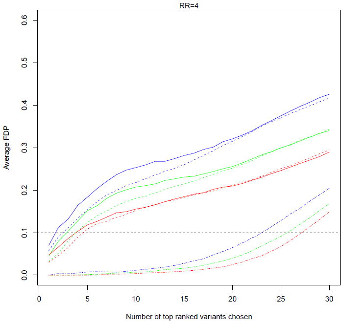
Underlining false discovery proportions under different configurations assuming RR=4: solid curves correspond to the hierarchical modeling approach while dashed curves correspond to the iBMU approach, both for the original WECARE configuration; two-dashed curves at the bottom of the graph correspond to the hierarchical modeling results for the WECARE 20 configuration (note that the iBMU approach was not implemented for WECARE 20 data for computational reasons); color of the curves indicates the sensitivity of the bioinformatic predictor: b = 0.7 (blue), b = 0.85 (green), and b = 0.95 (red); estimates are averaged across simulations.

Figure 4.

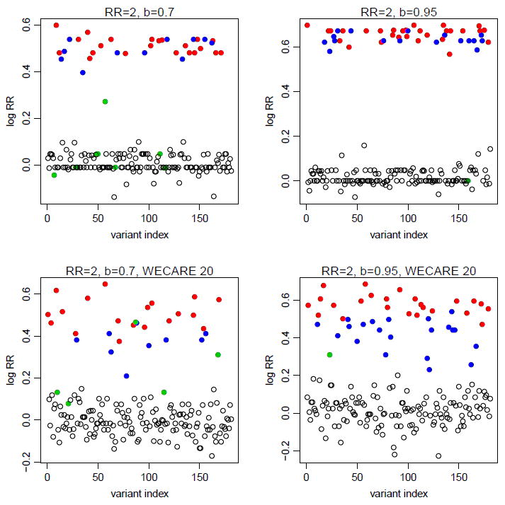
Estimated log relative risks for the 180 rare missense variants from one simulation assuming the original configuration of the WECARE data (top panels) or involving the denser WECARE 20 data (bottom panels) under the assumption that the relative risk of the truly deleterious variants was RR=2 and that b = 0.7 (left panels) or b = 0.95 (right panels); deleterious variants with positive bioinformatic predictor are depicted in red, neutral variants with positive bioinformatic predictor in blue, deleterious variants with negative bioinformatic predictor in green, and blank circles represent the neutral variants with negative bioinformatic predictor.

3.5.2 FDR Simulation Results

Recognizing that the underlining FDP is higher than desired in many of the configurations investigated, we examined the false discovery proportions and power obtained when applying two commonly used FDR controlling procedures (Benjamini-Hochberg and Efron’s local fdr) to the z-values produced by the hierarchical modeling approach. We also investigated the false discovery properties of the iBMU approach when the threshold of 3.2 was used for the MargBFs to declare significance of a specific variant. False discovery proportions and power estimates are provided in Table 1 for different magnitudes of the relative risk (RR) and different sensitivities of the bioinformatic predictor (represented by 100 × b%). In all cases the false discovery rate should be 10%. The methods have markedly disparate properties. The top part of Table 1 reports the results obtained when only one bioinformatic predictor is included in the second stage model. For small relative risks (RR=2), Benjamini-Hochberg barely makes any false discoveries but at the same time has essentially no power of finding truly deleterious variants either: rather than controlling the FDR at the desired threshold of 10%, the false discovery proportion is at most 2%, regardless of the accuracy of the bioinformatic predictor. On the other hand, Efron’s method severely underestimates the FDR in this setting, sometimes with almost half of the discoveries being false discoveries. For larger relative risks (RR=4), the Benjamini-Hochberg method achieves FDR control closer to the nominal threshold of 10%, though still with low power, while Efron’s locfdr has higher power but continues to yield inflated false discovery proportions. The performance of the iBMU approach was more similar to the hierarchical modeling approach with Efron’s approach used to control for multiple testing compared to when other multiple testing adjustments methods were used; it had somewhat lower false discovery proportions than Efron’s for most of the scenarios that assumed one bioinformatic predictor. Performing no adjustment also results in underestimated FDR in all configurations. Somewhat improved FDR control and power are observed with the inclusion of additional bioinformatic predictors as well as with increased accuracy of these predictors, though FDR control is still not achieved at the desired threshold (bottom of Table 1). As expected, the results are even worse when the proportion of truly deleterious variants is decreased from 15% to 10% (Supplementary Table 1) or when the accuracy of the bioinformatic predictors is decreased (Supplementary Table 2). In Figure 5 and Supplementary Figures 2 and 3, we plot the ROC curves constructed based on ranking on the z-values (solid curves) and based on ranking the MargBFs from the iBMU approach (dashed curves). The two approaches have similar ROC curves for the scenarios investigated. The curves and their area under the curves provide a graphical visualization of how the classification of the variants into deleterious versus neutral improves as the relative risks are increased, as well as the number of second stage predictors and their sensitivities. Note that the iBMU approach may have better performance in scenarios where the proportion of truly associated variants is low as the method uses a prior on the probability that each variant is associated that implicitly incorporates a multiplicity correction.

Table 1.

Power and FDP (expressed as percentages) for different magnitudes of relative risks (RR) and different associations with the bioinformatic predictors; 100×b% indicates the sensitivity of the bioinformatic predictor. 15% of variants are assumed to be truly deleterious. Theoretical FDR expected to be controlled at 10%.

(a) 1 bioinformatic predictor
	RR=2						RR=4
Method %	b=0.7		b=0.85		b=0.95		b=0.7		b=0.85		b=0.95
	Power	FDP	Power	FDP	Power	FDP	Power	FDP	Power	FDP	Power	FDP
No adjustment	17.3	20.9	27.6	21.0	35.0	24.1	42.9	28.0	61.7	30.4	73.9	29.1
BH FDR	1.9	0.9	3.3	1.1	4.9	1.7	15.4	7.5	25.9	10.1	37.7	12.7
local fdr	46.3	48.9	49.6	39.3	53.9	36.4	52.2	38.4	62.0	35.1	61.8	28.2
iBMU	41.7	40.4	51.0	34.8	57.0	33.7	58.6	35.9	73.4	33.3	82.3	30.7
(b) 3 bioinformatic predictors
No adjustment	30.3	19.2	40.6	16.5	45.3	20.1	64.7	25.3	78.5	22.8	90.9	18.5
BH FDR	2.7	0.6	6.5	0.7	9.0	0.7	28.5	6.0	46.3	5.8	63.9	4.8
local fdr	45.4	32.2	53.3	27.0	58.7	30.0	54.6	20.0	71.0	19.3	81.7	18.4
iBMU	39.8	35.2	42.6	33.1	41.9	33.1	68.1	29.1	78.1	24.5	87.1	20.5

Figure 5.

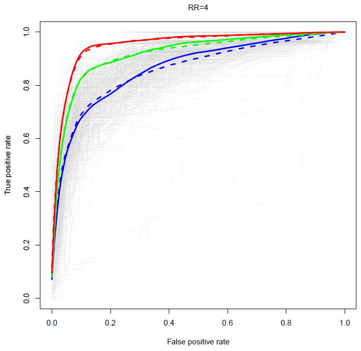
ROC curves of the z-values of the 180 rare missense variants (solid curves) and of the MargBF from the iBMU approach (dashed curves) under the assumption that the relative risk of the truly deleterious variants was RR=4; b = 0.7 (blue), b = 0.85 (green), and b = 0.95 (red); estimates are averaged across simulations.

With denser data (WECARE 20 fold), in settings with small relative risk (RR=2) and in which a single bioinformatic was included in the model, the proportion of false discoveries for the hierarchical modeling approach is still above the desired threshold (see Table 2). However, the performance is dramatically improved when the relative risks are higher (RR=4) or when additional bioinformatic predictors are included: both Benjamini-Hochberg and locfdr preserve the FDR at or below the nominal threshold with reasonable power that becomes closer to 100% as the sensitivity of the bioinformatic predictors is increased. For the scenario in which the sample size was increased so that variants carried by less than 10 subjects would occur in exactly 10 subjects, the performance is much improved compared to the sparse original WECARE data but expectedly poorer than for the much denser WECARE 20 fold scenario (see Supplementary Table 3). For computational reasons the iBMU approach was not implemented for these scenarios.

Table 2.

Power and FDP (expressed as percentages) for different magnitudes of relative risks (RR) and different associations with the bioinformatic predictors; 100 × b% indicates the sensitivity of the bioinformatic predictor; WECARE 20. 15% of variants are assumed to be truly deleterious. Theoretical FDR expected to be controlled at 10%. For computational reasons the iBMU approach was not implemented for these simulations.

(a) 1 bioinformatic predictor
	RR=2						RR=4
Method %	b=0.7		b=0.85		b=0.95		b=0.7		b=0.85		b=0.95
	Power	FDP	Power	FDP	Power	FDP	Power	FDP	Power	FDP	Power	FDP
No adjustment	67.7	26.9	80.9	28.9	93.0	30.8	91.9	25.4	95.3	26.4	98.0	28.0
BH FDR	29.9	7.0	44.8	10.8	67.3	17.3	73.5	4.5	84.8	7.1	92.2	11.4
local fdr	43.4	16.6	55.9	20.0	65.8	22.2	61.1	3.1	73.9	6.4	83.9	11.2
(b) 3 bioinformatic predictors
No adjustment	86.6	27.3	95.3	27.6	99.0	27.2	97.4	25.5	99.5	28.0	99.9	31.5
BH FDR	62.7	8.5	84.1	10.1	94.3	10.3	89.9	6.3	97.2	9.2	99.6	13.2
local fdr	61.8	10.2	82.2	11.9	93.0	12.4	83.2	4.1	94.4	6.9	98.2	9.0

To rule out that this performance is not a result of the idealized setup we studied in which the true risks of the variants assume only two different values, whereas the hierarchical model (2) involves a continuity of risk, we have also conducted simulations in which the log relative risks of the deleterious variants were generated from a normal distribution with mean β (β = log 2 and log 4) and standard deviation of 0.1 while the log relative risks of the neutral variants were generated from N(0, 0.1). As seen in Supplementary Tables 4 and 5, the results and conclusions are very similar for the hierarchical modeling approach.

Note the vastly different performances of the Benjamini-Hochberg and the Efron procedures even though they use the same test statistic as their input. One contributing factor to this difference is the estimated variance of the test statistic which can be considerably larger than the empirical variance. This leads to a very conservative test statistic resulting in the low false discovery rate as well as power of the Benjamini-Hochberg procedure as hardly any discoveries are made in certain configurations. Efron’s procedure alleviates this problem by replacement of the standard normal distribution with the empirical null distribution which results in more discoveries at the price of a larger false discovery proportion.

We have also studied the operating characteristics of several adaptations of Benjamini-Hochberg’s original FDR-controlling procedure (Benjamini and Hochberg 2000; Benjamini and Yekutieli 2001; Benjamini et al. 2006) and noted properties similar to the original procedure for the step-up procedures proposed by Benjamini and Hochberg (2000) and (Benjamini et al. 2006) but worse for the more conservative approach proposed by Benjamini and Yeku-tieli (2001) which provides FDR control under general dependency structures (data not shown).

In summary, it is critical that the bioinformatic predictor has high specificity and sensitivity in order for these methods to have valid false discovery properties. Increasing the sensitivity of the bioinformatic predictor improves the classification and the power, yet, unless the specificity is also increased, the number of false discoveries will still be larger than expected. Stronger relative risks also improve the power to distinguish the deleterious from neutral variants while controlling FDR at the nominal level.

4 Application to the WECARE BRCA1/BRCA2 data

We applied these methods to the WECARE Study based on the same hierarchical model as described in Capanu and Begg (2011). None of the 180 rare variants were declared significant at 0.1 threshold by the Benjamini-Hochberg method. This is not surprising in light of Figure 2 described in Section 2. Employing Efron’s locfdr approach identified 11 of the 180 variants as potentially harmful when using a locfdr threshold of 0.1 or below. The same 11 variants were deemed interesting when performing no multiple procedure adjustment and declaring significance based on p-values less than the threshold 0.1. They were also the top 11 ranked variants reported by Capanu et al. (2011) as being potentially promising and they were the sole 11 variants characterized by simultaneous adverse bioinformatic classifications on all three bioinformatic predictors (note that differences in results from the hierarchical modeling analysis based on 180 rare variants versus the analysis including 181 variants, as reported in Table IV of Capanu and Begg (2011), are negligible). The iBMU approach identified 21 variants as promising (with a MargBF ≥ 3.2) (see Supplementary Table 6), out of which 10 variants (denoted with a superscript “a” in the table) were common to the list of 11 variants discovered by the hierarchical modeling approach, while the other 11 variants (denoted with superscript “b” in the table) did not overlap with the list deemed interesting by the hierarchical modeling approach. Interestingly, most of these 11 non-overlapping variants occurred only in cases and had an adverse bioinformatic predictor for SIFT while their hierarchical modeling estimates ranged from 1.5 to 1.8.

5 Discussion

With the advent of next generation sequencing, the identification of disease loci when there are multiple rare variants is a cutting-edge issue in genetic epidemiology. There have been numerous recent methods developed with the purpose of identifying significant genes/loci (Li and Leal 2008; Morris and Zeggini 2010; Price et al. 2010; Ionita-Laza et al. 2011; Wu et al. 2011, among others) however they only provide indication of the global association of a particular gene/loci without being able to pinpoint which of the particular variants within the loci are driving the association. In previous work we have used hierarchical modeling techniques to estimate the relative risks of individual rare variants from a known risk gene, thus allowing us to make inference at the variant level. To the best of our knowledge, the integrative Bayesian uncertainty approach of Quintana and Conti (2013) is the only other alternative method that can pinpoint which of the individual variants within a risky loci is associated with disease. In this article we address the challenge of interpreting the results from these methods from the perspective of multiple testing. Using simulations we conclude that FDR control cannot be achieved in this framework unless the higher level covariate is very strongly predictive of the null/deleterious status of the variant and the magnitudes of the variants’ risks are large. There are currently no other methods to address this challenging problem. Conventional logistic regression would lead to infinite estimates for the singleton variants (which are typically the majority) or for variants that don’t occur in at least one case and one control, while for the other rare variants we showed that using hierarchical modeling provides a considerable efficiency boost over conditional logistic regression (Capanu and Begg 2011). By leveraging information using hierarchical modeling, one can prioritize the potentially high risk variants with the understanding that a significant number (depending on the accuracy of the higher level covariates and the magnitude of risk) will be false discoveries.

The simulations conducted show that when data are sparse, in this two class problem, the hierarchical modeling estimated risks of the null variants with high bioinformatic predictor values will be biased upwards and the risks of the deleterious variants with low bioinformatic predictor values will be shrank down resulting in the corresponding false positives and false negatives which in turn leads to higher false discovery rate and lower power respectively. Unless the higher level covariate has high sensitivity and specificity, in this rare variant setting, the shrinkage imposed by the hierarchical modeling structure leads to biased estimates and consequently to a high false discovery rate and low power. The performance improves with the addition of multiple independent informative higher level covariates. Furthermore, as the frequency of carriers increases, the model overrides the misclassifications of the higher level covariate, yielding less biased estimates and resulting in better classification properties. As the proportion of truly causal variants decreases, so does the performance of the methods. Similar behavior is expected for smaller sample sizes since in the absence of sufficient case-control frequencies, the hierarchical modeling approach will be even more heavily influenced by the higher level covariates.

The simulations we conducted were chosen to reflect a realistic setup even though by doing so the simulated data do not conform to the structure of the hierarchical model that we fit to the data. However note that even a correctly specified model (such as a mixture of generalized linear mixed models which is not feasible to fit for such sparse data) would suffer of the same limitations as observed here as a result of the shrinkage occurring due to the misspecification of the bioinformatic predictors.

Employing procedures that account for correlations between the test statistics would not remedy the FDR properties observed in our simulations. To support this argument, we take a close look here at the operating characteristics of the tests in this setting. For a given data set in the simulation the true deleteriousness state of the variants and the bioinformatic predictors are fixed and the case-control status is the only random variable. Now suppose we envision the distribution over all possible case-control vectors given by the variant frequencies and relative risks. That will in turn induce a distribution on the test statistics. The test of null is based on whether the observed test statistic exceeds the (FDR controlled) critical value derived from the marginal distribution. The test statistics under this distribution have minimal correlation although can be systematically biased depending on the combination of deleteriousness state and bioinformatic predictor. The statistics have minimal correlation because the variants occur in mutually exclusive subjects and the case-control status is generated independently for each subject. The issues with FDR control in this setting occur primarily due to the bias in the test statistic distributions and not due to correlated tests. Thus FDR control methods that account for correlation between the test statistics (discussed in the Introduction) do not have different FDR properties compared to the standard approach. Note that although the deleteriousness state vector is unknown, the operating characteristics depend only on the test statistic distribution conditioned on it.

Gelman’s argument that adjusting for multiple comparisons is not needed when multilevel models are employed does not apply in this setting in which the biased estimates and their over-estimated variances, as well as the departures from the standard normal distribution resulting from excessive shrinkage deteriorate the validity of the comparisons made with multilevel model estimates.

The hierarchical modeling approach had similar performance to the Bayesian integrative model uncertainty approach for the scenarios investigated. However the hierarchical modeling approach has the advantage of being computationally much faster (taking approximately 2 minutes to complete the analysis of a dataset on a single processor), while the Bayesian integrative approach can be extremely computationally intensive (which can take up to 1.5 hours to complete 100000 iterations for a single dataset on the same processor).

In summary, in this setting of testing multiple rare variants in the context of a random effects hierarchical model, the standard multiple testing procedures investigated do not achieve desired FDR control unless the higher level covariates have high accuracy in distinguishing deleterious from neutral variants and the strength of the relative risks of the variants is high. The FDR controlling procedures investigated trade off the power and FDR: if a more sensitive test is desired, one has to be willing to incur larger false discoveries than the prespecified threshold (Efron’s locfdr), whereas if the goal is to achieve better FDR control one has to be willing to use a less powerful test (Benjamini-Hochberg).

References

- Benjamini Y, Hochberg Y. Controlling the false discovery rate: a practical and powerful approach to multiple testing. Journal of the Royal Statistical Society. Series B. Methodological. 1995;57:289–300. [Google Scholar]
- Benjamini Y, Hochberg Y. On the adaptive control of the false discovery rate in multiple testing with independent statistics. Journal of Educational and Behavioral Statistics. 2000;25:60–83. [Google Scholar]
- Benjamini Y, Krieger AM, Yekutieli D. Adaptive linear step-up procedures that control the false discovery rate. Biometrika. 2006;93:491–507. [Google Scholar]
- Benjamini Y, Yekutieli D. The control of the false discovery rate in multiple testing under dependency. The Annals of Statistics. 2001;29:1165–1188. [Google Scholar]
- Bernstein JL, Langholz B, Haile RW, Bernstein L, Thomas DC, Stovall M, Malone KE, Lynch CF, Olsen JH, Anton-Culver H, Shore RE, Boice JD, Jr, Berkowitz GS, Gatti RA, Teitelbaum SL, Smith SA, Rosenstein BS, Borresen-Dale AL, Concannon P, Thompson WD. Study design: evaluating gene-environment interactions in the etiology of breast cancer - the WECARE Study. Breast Cancer Research. 2004;6:R199–R214. doi: 10.1186/bcr771. [DOI] [PMC free article] [PubMed] [Google Scholar]
- Blanchard G, Roquain E. Two simple sufficient conditions for FDR control. Electronic Journal of Statistics. 2008;2:963–992. [Google Scholar]
- Blanchard G, Roquain E. Adaptive FDR control under independence and dependence. Journal of Machine Learning Research. 2009;10:2837–2871. [Google Scholar]
- Borg A, Haile RW, Malone KE, Capanu M, Diep A, Töorngren T, Teraoka S, Begg CB, Thomas DC, Concannon P, Mellemkjaer L, Bernstein L, Tellhed L, Xue S, Olson ER, Liang X, Dolle J, Børresen-Dale AL, Bernstein JL. Characterization of BRCA1 and BRCA2 deleterious mutations and variants of unknown clinical significance in unilateral and bilateral breast cancer: the WECARE Study. Human Mutation. 2010;31:E1200–E1240. doi: 10.1002/humu.21202. [DOI] [PMC free article] [PubMed] [Google Scholar]
- Capanu M, Begg CB. Hierarchical Modeling for Estimating Relative Risks of Rare Genetic Variants: Properties of the Pseudo-Likelihood Method. Biometrics. 2011;67:371–380. doi: 10.1111/j.1541-0420.2010.01469.x. [DOI] [PMC free article] [PubMed] [Google Scholar]
- Capanu M, Concannon P, Haile RW, Olsen JH, Bernstein L, Malone KE, Lynch CF, Anton-Culver H, Liang X, Tellhed L, Teraoka SH, Diep AT, Thomas DC, Bernstein JL, Begg CB. Assessment of rare BRCA1 and BRCA2 variants of unknown significance using hierarchical modeling. Genetic Epidemiology. 2011;35:389–397. doi: 10.1002/gepi.20587. [DOI] [PMC free article] [PubMed] [Google Scholar]
- Capanu M, Gönen M, Begg CB. A hybrid Bayesian approach for generalized linear mixed models. Statistics in Medicine. 2012 doi: 10.1002/sim.5866. under review. [DOI] [PMC free article] [PubMed] [Google Scholar]
- Capanu M, Orlow I, Berwick M, Hummer AJ, Thomas DC, Begg CB. The use of hierarchical models for estimating relative risks of individual genetic variants: an application to a study of melanoma. Statistics in Medicine. 2008;27:1973–1992. doi: 10.1002/sim.3196. [DOI] [PMC free article] [PubMed] [Google Scholar]
- Clarke S, Hall P. Robustness of multiple testing procedures against dependence. The Annals of Statistics. 2009;37:332–358. [Google Scholar]
- Clyde M, George E. Model uncertainty. Statistical Science. 2004;19:81–94. [Google Scholar]
- Efron B. Large-scale simultaneous hypothesis testing: the choice of a null hypothesis. Journal of the American Statistical Association. 2004;99:96–103. [Google Scholar]
- Efron B. Correlation and large-scale simultaneous significance testing. Journal of the American Statistical Association. 2007a;102:93–103. [Google Scholar]
- Efron B. Size, power and false discovery rates. The Annals of Statistics. 2007b;35:1351–1377. [Google Scholar]
- Efron B. Correlated z-values and the accuracy of large-scale statistical estimates. Journal of the American Statistical Association. 2010;105:1042–1069. doi: 10.1198/jasa.2010.tm09129. [DOI] [PMC free article] [PubMed] [Google Scholar]
- Farcomeni A. Some results on the control of the false discovery rate under dependence. Scandinavian Journal of Statistics. 2007;34:275–297. [Google Scholar]
- Ge Y, Sealfon SC, Speed TP. Some step-down procedures controlling the false discovery rate under dependence. Statistica Sinica. 2008;18:881–904. [PMC free article] [PubMed] [Google Scholar]
- Gelman A, Hill J, Yajima M. Why we (usually) don’t have to worry about multiple comparisons. Technical Report Columbia University 2009 [Google Scholar]
- Genovese C, Roeder K, Wasserman L. False discovery control with p-value weighting. Biometrika. 2006;93:509–524. [Google Scholar]
- Genovese CR, Wasserman L. Operating characteristics and extensions of the false discovery rate procedure. Journal of the Royal Statistical Society. Series B. Methodological. 2002;64:499–517. [Google Scholar]
- Hoeting JA, Madigan D, Raftery AE, Volinsky CT. Bayesian model averaging: a tutorial (with discussion) Statistical Science. 1999;14:382–401. [Google Scholar]
- Ionita-Laza I, Buxbaum J, Laird N, Lange C. A new testing strategy to identify rare variants with either risk or protective effect on disease. PLoS Genetics. 2011;7:e1001289. doi: 10.1371/journal.pgen.1001289. [DOI] [PMC free article] [PubMed] [Google Scholar]
- Jeffreys H. Theory of Probability. 3 Oxford: Oxford Univ Press; 1961. [Google Scholar]
- Li B, Leal SM. Methods for detecting associations with rare variants for common diseases: application to the analysis of sequence data. American Journal of Human Genetics. 2008;83:311–321. doi: 10.1016/j.ajhg.2008.06.024. [DOI] [PMC free article] [PubMed] [Google Scholar]
- Li J, Ji L. Adjusting multiple testing in multilocus analyses using the eigenvalues of a correlation matrix. Heredity. 2005;95:221–227. doi: 10.1038/sj.hdy.6800717. [DOI] [PubMed] [Google Scholar]
- Li SS, Bigler J, Lampe JW, Potter JD, Feng Z. FRD-controlling testing procedures and sample size determination for microarrays. Statistics in Medicine. 2005;24:2267–2280. doi: 10.1002/sim.2119. [DOI] [PubMed] [Google Scholar]
- Morris AP, Zeggini E. An evaluation of statistical approaches to rare variant analysis in genetic association studies. Genetic Epidemiology. 2010;34:188–193. doi: 10.1002/gepi.20450. [DOI] [PMC free article] [PubMed] [Google Scholar]
- Ng PC, Henikoff S. Predicting deleterious amino acid substitutions. Genome Research. 2001;11:863–874. doi: 10.1101/gr.176601. [DOI] [PMC free article] [PubMed] [Google Scholar]
- Ng PC, Henikoff S. Accounting for human polymorphisms predicted to affect protein function. Genome Research. 2002;12:436–446. doi: 10.1101/gr.212802. [DOI] [PMC free article] [PubMed] [Google Scholar]
- Price AL, Kryukov GV, de Bakker PIW, Purcell SM, Staples J, Wei L, Sunyaev SR. Pooled association tests for rare variants in exon-resequencing studies. The American Journal of Human Genetics. 2010;86:832–838. doi: 10.1016/j.ajhg.2010.04.005. [DOI] [PMC free article] [PubMed] [Google Scholar]
- Quintana M. BVS: Bayesian Variant Selection: Bayesian Model Uncertainty Techniques for Genetic Association Studies. R package version 4.12.1 2012 [Google Scholar]
- Quintana MA, Bernstein JL, Thomas DC, Conti DV. Incorporating model uncertainty in detecting rare variants: the Bayesian risk index. Genetic Epidemiology. 2011;35:638–649. doi: 10.1002/gepi.20613. [DOI] [PMC free article] [PubMed] [Google Scholar]
- Quintana MA, Conti DV. Integrative variable selection via Bayesian model uncertainty. Statistics in Medicine. 2013;32:4938–4953. doi: 10.1002/sim.5888. [DOI] [PMC free article] [PubMed] [Google Scholar]
- Quintana MA, Schumacher FR, Casey G, Bernstein JL, Li L, Conti DV. Incorporating prior biologic information for high-dimensional rare variants association studies. Human Heredity. 2012;74:184–195. doi: 10.1159/000346021. [DOI] [PMC free article] [PubMed] [Google Scholar]
- Ramensky V, Bork P, Sunyaev S. Human non-synonymous SNPs: server and survey. Nucleic Acids Research. 2002;30:3894–3900. doi: 10.1093/nar/gkf493. [DOI] [PMC free article] [PubMed] [Google Scholar]
- Romano JP, Shaikh AM, Wolf M. Control of the false discovery rate under dependence using the bootstrap and subsampling. Test. 2008;17:417–442. [Google Scholar]
- Sarkar SK. Two-stage stepup procedures controlling FDR. Journal of Statistical Planning and Inference. 2008;138:1072–1084. [Google Scholar]
- Storey JD. A direct approach to false discovery rates. Journal of the Royal Statistical Society Series B Methodological. 2002;64:479–498. [Google Scholar]
- Storey JD. The optimal discovery procedure: a new approach to simultaneous significance testing. Journal of the Royal Statistical Society Series B Methodological. 2007;69:347–368. [Google Scholar]
- Storey JD, Tibshirani R. Technical Report 2001-28. Department of Statistics, Stanford University; CA: 2001. Estimating the positive False Discovery Rare under dependence with applications to DNA microarrays. [Google Scholar]
- Sunyaev S, Ramensky V, Bork P. Towards a structural basis of human non-synonymous single nucleotide polymorphisms. Trends in Genetics. 2000;16:198–200. doi: 10.1016/s0168-9525(00)01988-0. [DOI] [PubMed] [Google Scholar]
- Sunyaev S, Ramensky V, Koch I, Lathe W, III, Kondrashov AS, Bork P. Prediction of deleterious human alleles. Human Molecular Genetics. 2001;10:591–597. doi: 10.1093/hmg/10.6.591. [DOI] [PubMed] [Google Scholar]
- Tavtigian SV, Deffenbaugh AM, Yin L, Judkins T, Scholl T, Samollow PB, de Silva D, Zharkikh A, Thomas A. Comprehensive statistical study of 452 BRCA1 missense substitutions with classification of eight recurrent substitutions as neutral. Journal of Medical Genetics. 2006;43:295–305. doi: 10.1136/jmg.2005.033878. [DOI] [PMC free article] [PubMed] [Google Scholar]
- Wilson MA, Iversen E, Clyde MA, Schmidler SC, Schildkraut JM. Bayesian model search and multilevel inference for SNP association studies. The Annals of Applied Statistics. 2010;4:1342–1364. doi: 10.1214/09-aoas322. [DOI] [PMC free article] [PubMed] [Google Scholar]
- Wu MC, Lee S, Cai T, Li Y, Boehnke M, Lin X. Rare Variant Association Testing for Sequencing Data Using the Sequence Kernel Association Test (SKAT) American Journal of Human Genetics. 2011;89:82–93. doi: 10.1016/j.ajhg.2011.05.029. [DOI] [PMC free article] [PubMed] [Google Scholar]
- Yekutieli D. Hierarchical false discovery rate-controlling methodology. Journal of the American Statistical Association. 2008;103:309–316. [Google Scholar]
- Yekutieli D, Benjamini Y. Resampling-based false discovery rate controlling multiple test procedures for correlated test statistics. Journal of Statistical Planning and Inference. 1999;82:171–196. [Google Scholar]
- Zeisel A, Zuk O, Domany E. FDR control with adaptive procedures and FDR monotonicity. Annals of Applied Statistics. 2011;5:943–968. [Google Scholar]
Associated Data
This section collects any data citations, data availability statements, or supplementary materials included in this article.