Optimal full matching for survival outcomes: a method that merits more widespread use

Summary

Matching on the propensity score is a commonly used analytic method for estimating the effects of treatments on outcomes. Commonly used propensity score matching methods include nearest neighbor matching and nearest neighbor caliper matching. Rosenbaum (1991) proposed an optimal full matching approach, in which matched strata are formed consisting of either one treated subject and at least one control subject or one control subject and at least one treated subject. Full matching has been used rarely in the applied literature. Furthermore, its performance for use with survival outcomes has not been rigorously evaluated. We propose a method to use full matching to estimate the effect of treatment on the hazard of the occurrence of the outcome. An extensive set of Monte Carlo simulations were conducted to examine the performance of optimal full matching with survival analysis. Its performance was compared with that of nearest neighbor matching, nearest neighbor caliper matching, and inverse probability of treatment weighting using the propensity score. Full matching has superior performance compared with that of the two other matching algorithms and had comparable performance with that of inverse probability of treatment weighting using the propensity score. We illustrate the application of full matching with survival outcomes to estimate the effect of statin prescribing at hospital discharge on the hazard of post‐discharge mortality in a large cohort of patients who were discharged from hospital with a diagnosis of acute myocardial infarction. Optimal full matching merits more widespread adoption in medical and epidemiological research. © 2015 The Authors. Statistics in Medicine Published by John Wiley & Sons Ltd.

1. Introduction

There is an increasing interest in estimating the causal effects of treatments using observational (non‐randomized) data. Matching is an attractive analytic method to estimate the effect of treatments, due to its statistical properties and to the transparency and simplicity with which the results can be communicated. In matching, each treated or exposed subject is matched to one or more untreated or control subjects with similar covariate values. Outcomes are then compared between treatment groups in the matched sample. When using conventional matching methods, one is generally estimating the average effect of treatment in the treated (ATT): the effect of treatment in the sample or population of all subjects who were actually treated 1.

Pair‐matching involves the formation of pairs of treated and control subjects. Outcomes can then be compared between treated and control subjects in the matched sample. Pair‐matching, and matching in general, can be carried out on the basis of the covariates themselves (e.g., in Coarsened Exact Matching 2) or using a distance measure that combines information on multiple covariates, such as a Mahalanobis distance 3 or the propensity score 4. For the remainder of this paper, we will focus on matching on the propensity score, which is defined as the probability of treatment selection conditional on measured baseline covariates 5. Pair‐matching on the propensity score is frequently used in the medical literature 6, 7, 8. Alternative approaches that are used less frequently include many‐to‐one matching, in which each treated subject is matched to a fixed number of control subjects, and variable ratio matching, in which each treated subject is matched to a varying number of control subjects 9, 10. When using pair‐matching, there exist a large number of different algorithms to form the matched pairs. These include greedy nearest neighbor matching (NNM), NNM within fixed calipers, and optimal matching 11, 12. A recent study compared the performance of 12 different algorithms for pair‐matching 13. A limitation of caliper‐based pair‐matching algorithms is that some treated subjects may be excluded from the final matched sample because no appropriate control was found. Rosenbaum and Rubin coined the term ‘bias due to incomplete matching’ to refer to the bias that can occur when some treated subjects are excluded from the final matched sample because no appropriate control subject was found for those treated subjects 12. The occurrence of incomplete matching raises important issues around the generalizability of the estimated treatment effect. When incomplete matching occurs, frequently, it is those treated subjects who are the most likely candidates for therapy that are excluded from the matched sample (because of an insufficient number of control subjects who resemble the most likely candidates for therapy). In practice, incomplete matching occurs frequently in studies that use propensity score matching 14. Anecdotally, some clinical investigators are suspicious of pair‐matching because of its apparent wastefulness in not using the entire sample and its potential exclusion of a large number of control subjects from the analytic sample. A further limitation of conventional matching is that it requires a pool of potential controls that is substantially larger than the number of treated subjects. When the proportion of subjects that are treated is relatively large, conventional pair‐matching may not perform well. The reader is referred elsewhere for a more detailed discussion of different matching methods 4.

A rarely used alternative to the matching methods described earlier is full matching. Full matching involves the formation of strata consisting of either one treated subject and at least one control subject or one control subject and at least one treated subject 15, 16. An attractive feature of this approach is that it uses the entire sample; consequently, all treated subjects are included in the analysis. This method has been used rarely in the applied literature. Furthermore, its use has generally been restricted to settings with binary or continuous outcomes. Survival outcomes occur frequently in the medical and epidemiological literature 17. There are only a few examples of the use of full matching with survival outcomes 18, 19, 20, 21, and of these, only two used the Cox proportional hazards models. No papers have investigated the method in detail nor examined its performance across a variety of settings.

The objective of the current paper is to examine the estimation of marginal hazard ratios when using optimal full matching on the propensity score. The paper is structured as follows: In Section 2, we describe propensity scores and optimal full matching and propose a method to estimate the effect of treatment on survival outcomes when using full matching. In Section 3, we describe a series of Monte Carlo simulations to examine the performance of the proposed method for estimating marginal hazard ratios and to compare its performance to other, more frequently used approaches. In Section 4, we present the results of these Monte Carlo simulations. In Section 5, we present a case study in which we illustrate the application of these methods when estimating the effect of drug prescribing on the hazard of mortality in a cohort of patients discharged from hospital with a diagnosis of acute myocardial infarction. Finally, in Section 6, we summarize our findings and place them in the context of the existing literature.

2. Full matching and survival outcomes

In this section, we provide a description of propensity scores and optimal full matching. We then propose a method for estimating the effect of treatment on the hazard of the occurrence of an outcome when using full matching.

2.1. The propensity score

In an observational study of the effect of treatment on outcomes, the propensity score is the probability of receiving the treatment of interest conditional on measured baseline covariates: e= Pr(Z = 1|X), where X denotes the vector of measured baseline covariates 5. Four different propensity score methods have been described for reducing the effects of confounding when estimating treatment effects using observational data: matching, stratification, covariate adjustment, and inverse probability of treatment weighting (IPTW) 5, 22, 23. The reader is referred elsewhere for a broader overview of propensity score methods 24, 25.

2.2. Full matching

Rosenbaum used set‐theoretic terminology to define a stratification of a sample as follows 11. Let A denote the set of all treated subjects and B denote the set of all control subjects in the full sample. Then (A ₁,…,A _S,B ₁,…,B _S) denotes a stratification of the original sample that consists of S strata if the following conditions are met:

• $\left|A_i\right|\ge 1$ and $\left|B_i\right|\ge 1$ for i = 1,… ,S.

• A _s∩A _t=∅ and B _s∩B _t=∅ for s ≠ t.

• A ₁∪⋯∪A _S⊆A and B ₁∪⋯∪B _S⊆B.

Stratum s consists of the treated subjects from A _s and the control units from B _s, for s= 1,…,S. Note that, as specified in the third condition, it is not required that all subjects be included in the stratification.

Conventional propensity score‐based pair‐matching is a stratification in which |A _s|=|B _s|=1 for s = 1,…,S. It involves the formation of strata consisting of pairs of treated and control subjects, such that subjects in a matched pair have a similar value of the propensity score. Optimal pair‐matching forms pairs of treated and control subjects such that the average within‐pair difference in the propensity score (averaged across pairs) is minimized. Conventional stratification on the propensity score (e.g., as initially introduced by Rosenbaum and Rubin 5, 23) is a stratification such that A ₁∪⋯∪A _S=A and B ₁∪⋯∪B _S=B (hence, all subjects are included in one of the S strata). The strata in conventional propensity score stratification are often defined using specified quantiles (e.g., quintiles) of the propensity score 23.

Full matching is a stratification in which min(|A _s|,|B _s|) = 1 for s = 1,…,S. Thus, each stratum consists of either one treated subject and at least one control subject or one control subject and at least one treated subject. For a given sample, there will be multiple full matchings. An optimal full match is a full match that minimizes the mean within matched‐set differences in the propensity score between treated and control subjects. This is defined by Rosenbaum as follows 11. Let α=|A ₁∪⋯∪A _S| and β=|B ₁∪⋯∪B _S| denote the number of treated and control subjects in the stratification. Let δ(A _s,B _s) denote the average of the |A _s|×|B _s| distances between the |A _s| treated subjects and the |B _s| control subjects in stratum s (the distance is the difference between the propensity score of the treated subject and that of the control subject). For a given stratification, the distance associated with that stratification is defined as $\mathrm{\Delta }=\sum _{s=1}^{S}w\left(\right|A_s|,|B_s\left|\right)\delta (A_s,B_s)$, where w(|A _s|,|B _s|) is the weight associated with the given stratum. Rosenbaum suggested three different weight functions with which one could weight the mean stratum‐specific distances between treated and control subjects:

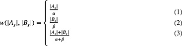
For a given weight function, an optimal full matching is a full matching that minimizes the distance Δ (note that for optimal pair‐matching, all three weight functions reduce to the reciprocal of the number of matched pairs). For the remainder of the paper, we will use the term full matching to refer to optimal full matching. Rosenbaum demonstrated that the problem of constructing an optimal full matching can be reduced to finding the minimum cost flow in a certain network 16. This is a combinatorial optimization problem for which algorithms currently exist. To gain an intuitive understanding of optimal full matching, one can think of it as rearranging already matched subjects between subclasses so as to minimize the average within‐stratum difference in the propensity score.

2.3. Survival analysis and full matching

In constructing a full matching stratification, each subject is assigned to a matched set consisting of either one treated subject and at least one control subject or one control subject and at least one treated subject. These matched sets are then used to create weights, allowing one to estimate the ATT. Treated subjects are assigned a weight of one. Each control subject has a weight proportional to the number of treated subjects in its matched set divided by the number of controls in the set 26, 27. For example, in a matched set with one control subject and three treated subjects, the control subject would be assigned a weight proportional to 3/1 = 3. In contrast, in a matched set with three control subjects and one treated subject, the control subject would be assigned a weight proportional to 1/3. The control group weights are scaled such that the sum of the control weights across all the matched sets is equal to the number of uniquely matched control subjects. All subjects in the original sample are contained in the sample created using full matching. Thus, the analytic sample is equivalent to the original sample. However, a stratification has been imposed on the sample, and weights have been assigned to each subject. The weights permit one to estimate the ATT, in that the weights weight the control subjects up to the distribution of treated subjects (an alternative fixed effects strategy for estimating linear treatment effects following full matching has been described by Hansen 15). We would like to highlight that the weights described in this section are different from those in the previous section. Those in the previous section were used as strata weights in defining an optimal full matching, while those in this section are estimation weights that permit estimation of the ATT.

Given a full matching in the context of survival outcomes, we propose that one estimates the effect of treatment on the hazard of the occurrence of the event by using a weighted Cox proportional hazards regression model to regress survival time on an indicator variable denoting treatment status. The model would incorporate the weights described previously. This approach is similar to how survey weights would be incorporated in a Cox proportional hazards model. The standard error of the estimated treatment effect can be estimated using a robust variance estimator that accounts for the clustering of subjects within the matched strata 28.

3. Monte Carlo simulations ‐ methods

We conducted a series of Monte Carlo simulations to examine the performance of optimal full matching to estimate marginal hazard ratios using a Cox proportional hazards model. We compared the performance of full matching with that of three other methods that permit estimation of the ATT: (i) NNM; (ii) nearest neighbor caliper matching; and (iii) IPTW using the propensity score with ATT weights. We did not consider conventional stratification on the quintiles of the propensity score, as previous research has shown that this method does not perform well for estimating marginal hazard ratios 29. We assessed the performance of each method using the following criteria: (i) the degree to which matching reduced the observed differences in baseline covariates between treatment groups; (ii) bias in estimating the true marginal hazard ratio; (iii) the variability of the estimated hazard ratios; (iv) the accuracy of the estimated standard error of the estimated treatment effect; (v) the mean squared error (MSE) of the estimated log‐hazard ratio; (vi) the empirical coverage rates of nominal 95% confidence intervals (CIs); and (vii) whether the empirical type I error rate was equal to the advertised rate when there was a true null treatment effect.

We examine three different scenarios. In the first, which was intended as our primary analysis, we considered the case in which all baseline covariates were continuous and in which the effect of confounding was moderate. The second scenario was a modification of the first, in which the effect of confounding was strong. The third scenario was a case in which the large majority of baseline covariates were dichotomous and the effect of confounding was moderate.

3.1. Data‐generating process

The design of our Monte Carlo simulations was similar to those used in earlier studies to examine the different aspects of propensity score analysis 13, 29, 30, 31, 32, 33, 34, 35. As in these prior studies, we assumed that there were ten covariates (X₁–X₁₀), generated from independent standard normal distributions, which each effected either treatment selection and/or the outcome. The treatment–selection model was logit(p _i,treat) = β _0,treat+β _W x _1,i+β _W x _2,i+β _M x _4,i+β _M x _5,i+β _S x _7,i+β _S x _8,i+β _VS x _10,i. For each subject, treatment status (denoted by z) was generated from a Bernoulli distribution with parameter p _i,treat. The intercept of the treatment–selection model (β _0,treat) was selected so that the proportion of subjects in the simulated sample that were treated was fixed at the desired proportion (5%, 10%, 20%, 30%, 40%, and 50%). The regression coefficients β _W, β _M, β _S, and β _VS were set to log(1.25), log(1.5), log(1.75), and log(2), respectively. These were intended to denote weak, moderate, strong, and very strong treatment–assignment affects. Thus, seven covariates affected treatment selection, and there were four different magnitudes for the effect of a covariate on the odds of receiving the treatment.

A time‐to‐event outcome was generated for each subject using a data‐generating process for survival outcomes described by Bender et al. 36. For each subject, the linear predictor was defined as

$$\begin{array}{c}\text{LP}={\alpha }_{\text{treat}}z+{\alpha }_W{x}_2+{\alpha }_W{x}_3+{\alpha }_M{x}_5+{\alpha }_M{x}_6+{\alpha }_S{x}_8+{\alpha }_S{x}_9+{\alpha }_{\mathrm{VS}}{x}_{10}+\\ z{\alpha }_W{x}_2+z{\alpha }_M{x}_5+z{\alpha }_S{x}_8+z{\alpha }_{\mathrm{VS}}{x}_{10}\\ \end{array}$$

The regression coefficients α _W, α _M, α _S, and α _VS (denoting log‐hazard ratios) were set to log(1.25), log(1.5), log(1.75), and log(2), respectively. The inclusion of interactions between treatment status (Z) and the four confounding variables (X₂, X₅, X₈, and X₁₀) was intended to induce treatment‐effect heterogeneity, so that the effect of treatment depended on the values of these covariates. For each subject, we generated a random number from a standard Uniform distribution: u ~U(0,1). A survival or event time was generated for each subject as follows: ${\left(\frac{-\log \left(u\right)}{\lambda e^{\text{LP}}}\right)}^{{}^{1/\eta }}$. We set λ and η to be equal to 0.00002 and 2, respectively. The use of this data‐generating process results in a conditional treatment effect, with a conditional hazard ratio of exp(α _treat). However, we wanted to generate data in which there was a specified marginal hazard ratio. To do so, we modified previously described data‐generating processes for generating data with a specified marginal odds ratio or risk difference 37, 38. We used an iterative process to determine the value of α _treat (the conditional log‐hazard ratio) that induced the desired marginal hazard ratio. Briefly, using the aforementioned conditional model, we simulated a time‐to‐event outcome for each subject, first assuming that the subject was untreated and then assuming that the subject was treated. In the sample consisting of both potential outcomes (survival or event time under lack of treatment and survival or event time under treatment) for those subjects who were ultimately assigned to treatment, we regressed the survival outcome on an indicator variable denoting treatment status. The coefficient for the treatment status indicator denotes the log of the marginal hazard ratio. We repeated this process 1000 times to obtain an estimate of the log of the marginal hazard ratio associated with a specific value of α _treat in our conditional outcomes model. A bisection approach was then employed to determine the value of α _treat, which resulted in the desired marginal hazard ratio. This process was performed using only those subjects who were ultimately assigned to the treatment (i.e., we fit the Cox model on the dataset of potential outcomes restricted to those subjects who were ultimately treated) as we were determining the value of α _treat that induced a desired marginal hazard ratio in the treated population (ATT). Such an approach has been used in previous studies 29, 39. R code for implementing a data‐generating process similar to the one described earlier is provided in an appendix in a recently‐published paper by the first author 35.

The aforementioned set of odds ratios (for treatment assignment) or hazard ratios (for the hazard of the outcome) (1.25, 1.5, 1.75, and 2) was selected to represent odds ratios or hazard ratios that are reflective of those in many epidemiological and medical contexts (for instance, in the EFFECT‐HF mortality prediction model, a one standard deviation increase in age was associated with an odds ratio of 1.81 for 30‐day mortality in patients hospitalized with heart failure, while a one standard deviation increase in respiratory rate was associated with an odds ratio of 1.34. A one standard deviation decrease in systolic blood pressure was associated with an odds ratio of 1.78 40). Our Monte Carlo simulations had a factorial design in which the proportion of subjects that were treated took on the following six values: 0.05, 0.10, 0.20, 0.30, 0.40, and 0.50. In each of the six scenarios, we simulated 1000 datasets, each consisting of 1000 subjects. We do not anticipate that NNM will perform well in settings in which the prevalence of treatment is 0.40 or 0.50. In such settings, the pool of potential controls is, at most, modestly larger than the number of treated subjects. Thus, it will be difficult to identify high‐quality matches for all treated subjects, leading to residual imbalance and confounding. An applied analyst would not be advised to use NNM in these scenarios. We included these scenarios in order to examine the performance of full matching in settings in which NNM would be expected to perform poorly.

3.2. Statistical analyses in simulated datasets

3.2.1. Estimation of regression coefficients, standard errors, and confidence intervals

In each simulated dataset, we estimated the propensity score using a logistic regression model to regress treatment assignment on the seven variables that affect the outcome, as this approach has been shown to result in superior performance compared with including all measured covariates or those variables that affect treatment selection 41.

In each simulated dataset, an optimal full matching was created using the estimated propensity score. In the full sample, the hazard of the occurrence of the outcome was regressed on an indicator variable denoting treatment selection using a Cox proportional hazards model with the weights described previously. Two different methods were used to estimate the variance of the treatment effect. First, as proposed earlier, a robust sandwich‐type variance estimator was used, which accounted for the clustering of subjects within subclasses or strata 28. Second, to examine the consequences of not using a robust variance estimator, the naïve model‐based standard errors obtained from the maximum partial likelihood estimation were obtained. We refer to these two approaches as the robust approach and the naïve approach, respectively.

Three methods were used as comparators for the performance of full matching. First, greedy NNM without replacement was used to match each treated subject to the control subject whose propensity score was closest to that of the treated subject. Second, nearest neighbor caliper matching without replacement was used to match each treated subject to a control subject. Subjects were matched on the logit of the propensity score using a caliper of width equal to 0.2 of the standard deviation of logit of the propensity score. This caliper width was selected as it has been shown to often result in estimates with the lowest MSE compared with the use of other caliper widths 42. The treated subject was matched to the closest control subject whose logit of the propensity score lay within the specified caliper distance of that of the treated subject. Third, IPTW was used with ATT weights (we refer to this as IPTW‐ATT). If e denotes the estimated propensity score, then the original sample was weighted by the following weights: $Z+\frac{(1-Z)e}{1-e}$ (i.e., treated subjects were assigned a weight of 1, while control subjects were assigned a weight of $\frac{e}{1-e})$. These ATT weights are sometimes referred to as ‘weighting by the odds’ or ‘treatment on the treated’ weights. With the two pair‐matching approaches, a Cox proportional hazards model was estimated in the matched sample to regress the hazard of the occurrence of the outcome on an indicator variable denoting treatment selection. A robust, sandwich‐type variance estimator that accounted for the matched‐pair design was used to estimate the sampling variability of the estimated treatment effect 28, 29. For the IPTW‐ATT approach, the hazard of the occurrence of the event of interest was regressed on an indicator variable denoting treatment status, as with full matching, but where the weights used in estimating this model were the IPTW‐ATT weights. Again, a robust variance estimator was used 28, 43.

Apart from NNM and caliper matching, which were implemented using custom‐written programs in the C programming language, all other analyses were conducted in the R statistical programming language (version 3.0.2). Full matching was implemented using the matchit function from the MatchIt package (R Foundation for Statistical Computing, Vienna, Austria) (version 2.4‐21) 26, 27. The weights for use with full matching were those generated by the matchit function. Both NNM and caliper matching can be implemented using matchit; we elected to use C implementation of these two algorithms for consistency with previously published work by the first author and for computational efficiency in the simulations.

Let θ denote the true treatment effect on the log‐hazard ratio scale (= log(0.8)), and let θ _i denote the estimated treatment effect, also on the log‐hazard ratio scale, in the i‐th simulated sample (i= 1,…,1000). Then, the mean estimated log‐hazard ratio was estimated as $\frac{1}{1000}\sum _{i=1}^{1000}{\theta }_i$, and the MSE was estimated as $\frac{1}{1000}\sum _{i=1}^{1000}{({\theta }_i-\theta )}^2$. Ninety‐five per cent CIs were constructed for each estimate of the treatment effect, and the proportion of CIs that contained the true measure of effect was determined. The mean estimated standard error of the estimated treatment effect was computed across the 1000 simulated datasets. This quantity was compared with the standard deviation of the estimated treatment effects (on the log‐hazard ratio scale) across the 1000 simulated datasets. If the estimated standard error is, on average, correctly approximating the sampling variability of the estimated treatment effect, the ratio of these two quantities should be approximately one.

The propensity score is a balancing score 5. Accordingly, we also compared the ability of the three different matching methods to balance measured baseline confounding variables between treated and control subjects. In each of the matched samples, standardized differences were computed, comparing the mean of each covariate between the treated and control subjects 44. When using full matching, the computation of the means and variances necessary for computing the standardized differences incorporated the weights described earlier. Thus, weighted means and weighted variances were calculated. For each of the 10 covariates, the mean standardized difference was calculated across the 1000 simulated datasets.

3.2.2. Estimating the empirical type I error rate

We repeated the simulations mentioned earlier using a true null marginal hazard ratio (equivalent to allowing α _treat to be equal to zero in the data‐generating process). We then conducted analyses similar to those described previously. In each simulated dataset and using each statistical method, we noted the statistical significance of the estimated effect of treatment (using a significance level of 0.05 to denote statistical significance). We then estimated the empirical type I error rate as the proportion of simulated datasets in which the null hypothesis was rejected.

3.2.3. Examining the impact of increased confounding

In the simulations described earlier, the odds ratios relating the baseline covariates to the odds of treatment assignment were low to modest: 1.25, 1.5, 1.75, and 2. These were chosen to reflect values typical of those in many medical or epidemiological settings in which the degree of confounding is moderate. To examine the effect of a more extreme degree of confounding, we repeated the previous simulations with these treatment odds ratios increased to 2, 3, 4, and 5, respectively. This would have the impact of increasing the covariate separation between the treated and control subjects in the full sample.

3.2.4. Examining scenarios with binary covariates

In the aforementioned scenarios, the 10 baseline covariates were continuous. In many epidemiological settings, some of the baseline covariates may be dichotomous, representing the presence or absence of binary risk factors (e.g. presence or absence of diabetes). We repeated the analyses conducted under moderate confounding in scenarios in which nine of the 10 covariates were binary. In the data‐generating process described previously, X₁ to X₉ were simulated from independent Bernoulli random variables, each with parameter 0.5. As age, a continuous variable, is often a confounding variable, X₁₀ remained a continuous variable with a standard normal distribution in the data‐generating process.

4. Monte Carlo simulations – results

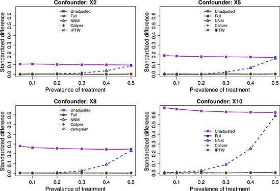
The balance induced on the four confounding variables, as measured using standardized differences, is described in Figures 1 (scenarios with moderate confounding) and 2 (scenarios with strong confounding). In each figure, there is one panel for each of the four confounding variables (X₂, X₅, X₈, and X₁₀). For comparative purposes, we also report the crude imbalance in the original, unmatched sample. By examining the imbalance in the original unmatched sample, one can quantify the initial degree of confounding (imbalance) that was present in the four confounding variables. To place these numbers in context, some authors use a threshold of 0.10 (10%) to indicate potentially meaningful imbalance 45. Full matching, caliper matching, and IPTW induced essentially perfect balance on the confounding variables. The residual imbalance observed for NNM increased with increasing prevalence of treatment. The explanation for this last observation is that as the prevalence of treatment increases, the pool of potential controls decreases in size. NNM does not place a constraint on the quality of the match. Thus, as the pool of potential controls decreases in size, treated subjects are increasingly being matched to more dissimilar subjects, resulting in greater residual imbalance.

Figure 1.

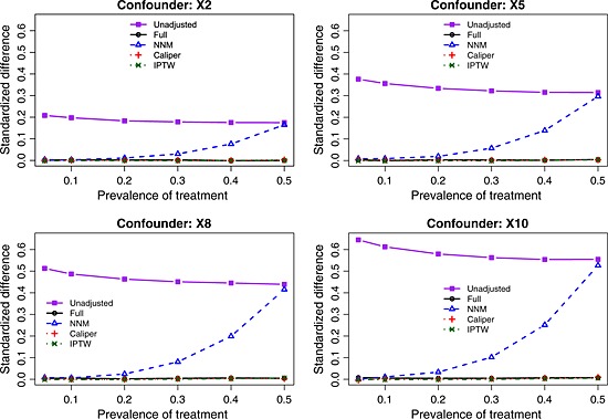
Standardized differences for the four confounding variables (moderate confounding). NNM, nearest neighbor matching; IPTW, inverse probability of treatment weighting.

Figure 2.

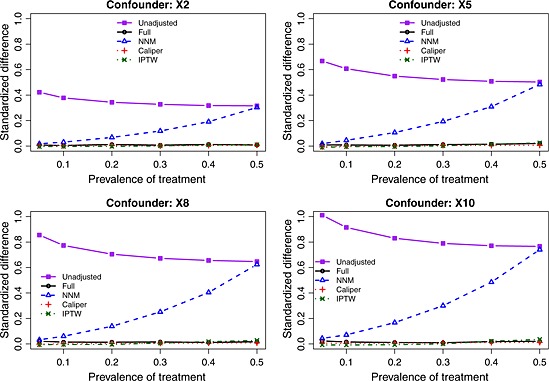
Standardized differences for the four confounding variables (strong confounding). NNM, nearest neighbor matching; IPTW, inverse probability of treatment weighting.

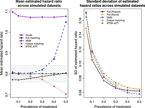
The exponential of the mean estimated log‐hazard ratio across the 1000 simulated datasets for each scenario and each estimation method are reported in Figure 3 (note that we computed the mean log‐hazard ratio across the 1000 simulations and we report the exponential of this quantity for ease of interpretation and for the ability to compare it with the true value of 0.8). There are two panels in this figure. The left panel denotes the results for the setting with moderate confounding, while the right panel denotes the results for the setting with strong confounding. We have superimposed on this figure a solid horizontal line denoting the true treatment effect (a hazard ratio of 0.8) and a shaded area denoting a relative bias of at most 5%. We also report the mean estimated log‐hazard ratio when using the crude or unadjusted estimator. This was added to allow for an appreciation for the magnitude of the degree of bias in the original sample. When using full matching, we observe that the relative bias is always less than 5%. Furthermore, the magnitude of the bias decreases as the prevalence of treatment increases to 50%. The use of IPTW‐ATT resulted in essentially unbiased estimation, regardless of the prevalence of treatment. Both pair‐matching approaches resulted in estimates with a relative bias that exceeded 5% when the prevalence of treatment exceeded 30% (moderate confounding) or 10% (strong confounding). For both pair‐matching approaches, the magnitude of the bias increased with increasing prevalence of treatment.

Figure 3.

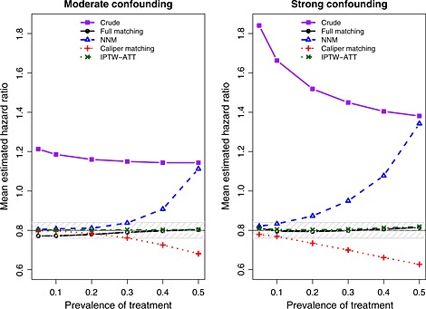
Mean estimated hazard ratio across simulated datasets. NNM, nearest neighbor matching; IPTW, inverse probability of treatment weighting; ATT, average effect of treatment in the treated.

The standard deviation of the estimated log‐hazard ratios across the 1000 simulated datasets is described in Figure 4. Full matching (with robust variance estimation when confounding was moderate and with the naïve variance estimate when confounding was strong) tended to result in estimates that displayed the least variability, whereas IPTW‐ATT tended to result in estimates that displayed the greatest variability. When confounding was moderate, the ratio of the standard error from IPTW‐ATT to that of full matching (with robust variance estimation) decreased from 1.14 to 1.02 as the prevalence of treatment increased, while the absolute difference in standard errors between the two methods decreased from 0.021 to 0.002. Thus, while some methods displayed greater variability in estimates than other methods, the differences were, at most, modest.

Figure 4.

Standard deviation (SD) of estimated hazard ratios across simulated datasets. NNM, nearest neighbor matching; IPTW, inverse probability of treatment weighting; ATT, average effect of treatment in the treated.

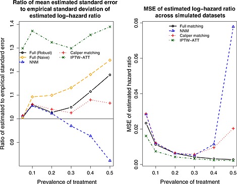
The ratio of the mean estimated standard error of the estimated log‐hazard ratio to the standard deviation of the estimated log‐hazard ratios is reported in Figure 5. A horizontal line denoting a ratio of one has been superimposed on this figure. When comparing robust variance estimation for full matching with the use of a naïve variance estimator for full matching, one observes that the robust approach resulted in a ratio that was closer to unity in the presence of moderate confounding, indicating that the estimated standard errors of the log‐hazard ratios were more closely approximating the standard deviation of the sampling distribution of the estimated log‐hazard ratios. However, the converse was observed in the presence of strong confounding. In the presence of moderate confounding, the mean estimated standard error of the IPTW‐ATT estimate of the log‐hazard ratio was approximately 50% higher than the empirical standard deviation of the estimated log‐hazard ratio. Thus, IPTW‐ATT resulted in estimates of the standard error of the estimated log‐hazard ratio that tended to be consistently worse than those of the other methods. We speculate that the explanation for this poor performance may relate to the presence of extreme weights. Further research in variance estimation for propensity score methods is merited.

Figure 5.

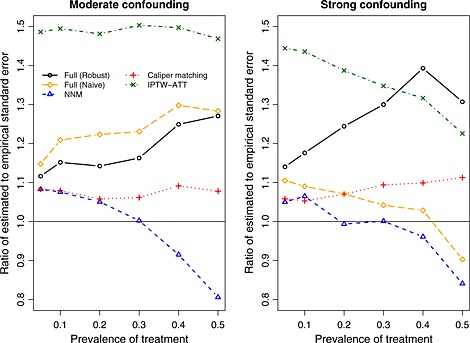
Ratio of mean estimated standard error to empirical standard deviation of the estimated log‐hazard ratio. NNM, nearest neighbor matching; IPTW, inverse probability of treatment weighting; ATT, average effect of treatment in the treated.

The MSE of the estimated log‐hazard ratios across the 1000 simulated datasets for each scenario is reported in Figure 6. The use of IPTW‐ATT resulted in estimates with the lowest MSE. However, differences between full matching and IPTW‐ATT diminished as the prevalence of treatment increased. The MSE of the two pair‐matching approaches resulted in estimates with the greatest MSE. Differences between the two pair‐matching approaches and the other two approaches were amplified as the prevalence of treatment increased, reflecting the increase in bias observed earlier.

Figure 6.

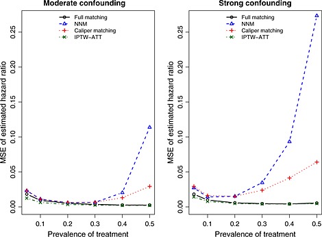
Mean squared error (MSE) of estimated hazard ratio across simulated datasets. NNM, nearest neighbor matching; IPTW, inverse probability of treatment weighting; ATT, average effect of treatment in the treated.

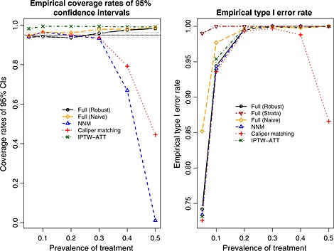
Empirical coverage rates of estimated 95% CIs are reported in Figure 7. A horizontal line denoting the advertised coverage rate of 0.95 has been superimposed on the figure. A shaded region denoting empirical coverage rates between 0.9365 and 0.9635 has been added in the figure. Given our use of 1000 simulated datasets, empirical coverage rates lower than 0.9365 or greater than 0.9635 would be statistically significantly different from 0.95, using a standard normal‐theory test. In general, all methods had suboptimal coverage. Full matching (both using the robust approach and the naïve approach) resulted in CIs with elevated coverage rates. In the presence of strong confounding, the performance of full matching with the naïve variance estimator improved as the prevalence of treatment increased. Similarly, IPTW‐ATT resulted in estimated CIs whose empirical coverage rates were significantly higher than the advertised rate. Both pair‐matching approaches resulted in methods with satisfactory coverage rates when the prevalence of treatment was low. However, coverage rates dropped precipitously when the prevalence of treatment was high.

Figure 7.

Empirical coverage rates of 95% confidence intervals (CIs). NNM, nearest neighbor matching; IPTW, inverse probability of treatment weighting; ATT, average effect of treatment in the treated.

The empirical type I error rates are reported in Figure 8. A horizontal line denoting the advertised type I error rate (0.05) has been superimposed on the figure. A shaded area denoting type I error rates between 0.0365 and 0.0635 has been superimposed on the figure. Given our use of 1000 simulated datasets, empirical type I error rates below 0.0365 or above 0.0635 would be statistically significantly different from 0.05 using a standard normal‐theory test. In examining Figure 8, one observes that no method had uniformly good performance. However, the performance of full matching and IPTW‐ATT improved as the prevalence of treatment increased.

Figure 8.

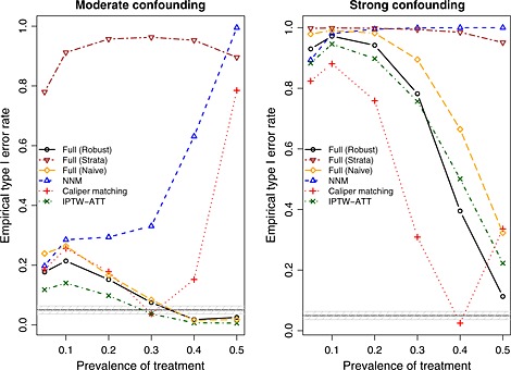
Empirical type I error rates. NNM, nearest neighbor matching; IPTW, inverse probability of treatment weighting; ATT, average effect of treatment in the treated.

Results for the scenarios with moderate confounding in which nine of the covariates were binary are reported in Figures 9, 10, 11, 12. Results comparable with those described earlier for the scenarios with moderate confounding and solely continuous covariates were observed.

Figure 9.

Mixed covariates: standardized differences for the four confounding variables. NNM, nearest neighbor matching; IPTW, inverse probability of treatment weighting.

Figure 10.

Mixed covariates: mean and standard deviation of estimated hazard ratios across simulated datasets. NNM, nearest neighbor matching; IPTW, inverse probability of treatment weighting; ATT, average effect of treatment in the treated.

Figure 11.

Mixed covariates: empirical versus estimated standard error and mean squared error (MSE). NNM, nearest neighbor matching; IPTW, inverse probability of treatment weighting; ATT, average effect of treatment in the treated.

Figure 12.

Mixed covariates: empirical coverage rates of 95% confidence intervals (CIs) and empirical type I error rates. NNM, nearest neighbor matching; IPTW, inverse probability of treatment weighting; ATT, average effect of treatment in the treated.

5. Case study

Data were available on 9107 patients discharged from 103 acute care hospitals in Ontario, Canada, with a diagnosis of acute myocardial infarction (acute myocardial infarction or heart attack) between April 1, 1999 and March 31, 2001. These subjects were included in the Enhanced Feedback for Effective Cardiac Treatment (EFFECT) Study, an initiative intended to improve the quality of care for patients with cardiovascular disease in Ontario 46, 47. Data on patient demographics, vital signs and physical examination at presentation, medical history, and results of laboratory tests were collected for this sample. Baseline characteristics of the study sample, when stratified by the treatment variable, are reported in Table 1. These data were used in a recently published tutorial on the use of propensity score methods for the analysis of survival data 48. Full matching was not examined in this earlier tutorial; however, we replicate some of the previously conducted analyses to compare with the use of full matching. The reader is referred to the prior publication for additional details.

Table 1.

Comparison of baseline characteristics between treated and untreated subjects in the sample used for the case study.

	Original sample
Baseline variable	Statin: no (6058)	Statin: yes (3049)	Standardized difference
Demographic characteristics
Age (years)	68.1 ± 13.8	63.4 ± 12.4	0.355
Female	2241 (37.0%)	887 (29.1%)	0.167
Presenting signs and symptoms
Acute congestive heart failure/pulmonary edema	316 (5.2%)	122 (4.0%)	0.057
Classic cardiac risk factors
Family history of heart disease	1763 (29.1%)	1177 (38.6%)	0.204
Diabetes	1562 (25.8%)	774 (25.4%)	0.009
Hyperlipidemia	1138 (18.8%)	1761 (57.8%)	0.910
Hypertension	2683 (44.3%)	1453 (47.7%)	0.068
Current smoker	2004 (33.1%)	1070 (35.1%)	0.043
Cardiac history and comorbid conditions
CVA/TIA	610 (10.1%)	237 (7.8%)	0.079
Angina	1871 (30.9%)	1086 (35.6%)	0.101
Cancer	191 (3.2%)	73 (2.4%)	0.045
Dementia	243 (4.0%)	33 (1.1%)	0.171
Previous AMI	1254 (20.7%)	799 (26.2%)	0.132
Asthma	338 (5.6%)	166 (5.4%)	0.006
Depression	441 (7.3%)	192 (6.3%)	0.039
Hyperthyroidism	71 (1.2%)	40 (1.3%)	0.013
Peptic ulcer disease	345 (5.7%)	156 (5.1%)	0.025
Peripheral vascular disease	430 (7.1%)	220 (7.2%)	0.005
Previous coronary revascularization	433 (7.1%)	411 (13.5%)	0.220
Congestive heart failure (chronic)	275 (4.5%)	91 (3.0%)	0.079
Stenosis	96 (1.6%)	35 (1.1%)	0.037
Vital signs on admission
Systolic blood pressure	148.7 ± 31.6	149.3 ± 30.1	0.021
Diastolic blood pressure	83.6 ± 18.6	84.5 ± 18.0	0.047
Heart rate	84.6 ± 24.3	81.7 ± 23.0	0.121
Respiratory rate	21.2 ± 5.7	20.3 ± 4.8	0.166
Results of initial laboratory tests
White blood count	10.3 ± 4.9	10.0 ± 4.4	0.065
Hemoglobin	137.5 ± 19.3	140.6 ± 16.9	0.167
Sodium	138.9 ± 3.9	139.2 ± 3.3	0.079
Glucose	9.4 ± 5.1	9.2 ± 5.3	0.037
Potassium	4.1 ± 0.6	4.1 ± 0.5	0.061
Creatinine	105.7 ± 65.4	99.9 ± 50.0	0.096

AMI, acute myocardial infarction; CVA,; TIA,.Note: Continuous variables are reported as means±standard deviations. Dichotomous variables are reported as N (%). Table reproduced from 48.

For the current case study, the exposure of interest was whether the patient received a prescription for a statin lipid‐lowering agent at hospital discharge. Three thousand and forty‐nine (33.5%) patients received a statin prescription at hospital discharge. The outcome of interest for this case study was time from hospital discharge to death. Patients were censored after 8years of follow‐up. Three‐thousand five hundred and ninety‐three (39.5%) patients died within 8years of hospital discharge.

The matchit function that was used in the Monte Carlo simulations for constructing an optimal full matching imposes a maximum size on the distance matrix that describes the distance (difference in propensity scores) between each treated and control subject. Because of this constraint and the large sample size, we were unable to use the matchit function for the case study. Newer versions of the fullmatch function from the optmatch package 49 do not have this constraint. Thus, for the purposes of the case study, we used fullmatch (from optmatch version 0.9‐3).

A propensity score for statin treatment was estimated using logistic regression to regress an indicator variable denoting statin treatment on 31 baseline covariates. Restricted cubic splines were used to model the relationship between each of the 11 continuous covariates and the log odds of treatment. Each of the methods described earlier was used to estimate the effect of statin prescribing at discharge on the hazard of mortality. Based on the results of our simulations, a robust variance estimator that accounted for the stratification was used with full matching.

After constructing the full match stratification of the sample, the standardized differences for the 31 baseline covariates ranged from −0.044 to 0.066. When using NNM, the standardized differences ranged from −0.046 to 0.424, while when using caliper matching, they ranged from −0.028 to 0.037. Thus, the estimate obtained using NNM is likely to be contaminated by a modest degree of residual confounding. When using NNM, the large standardized difference of 0.424 was for the variable denoting a history of hyperlipidemia – a key variable influencing statin prescribing. Apart from hyperlipidemia, the largest standardized difference when using NNM was 0.080. While caliper matching induced good balance in the 31 measured baseline covariates, it resulted in the exclusion of 21% of the treated subjects. Thus, the estimate of the ATT obtained using caliper matching may be subject to bias due to incomplete matching.

When using full matching, the estimated hazard ratio was 0.901 (95% CI: (0.816, 0.994)), which was statistically significantly different from the null (P = 0.038). The estimate obtained using IPTW‐ATT was slightly larger: 0.927 (95% CI: (0.846, 1.016); P = 0.106). The use of NNM resulted in an estimated hazard ratio of 0.914 (95% CI: (0.838, 0.997); P = 0.044). When using caliper matching, 2422 (79%) of the 3049 patients prescribed a statin were successfully matched to a control subject. The resultant hazard ratio was 0.868 (95% CI: (0.791, 0.953); P = 0.003).

While the two estimated hazard ratios obtained using full matching and IPTW‐ATT were qualitatively similar to one another, which was consistent with the results of our simulations, they differed in their statistical significance (P < 0.05 vs. P > 0.05). NNM and caliper matching resulted in estimates of the effect of statin of greater magnitude. The estimated obtained using caliper matching may be contaminated by bias because of incomplete matching due to the exclusion of 21% of the treated subjects.

6. Discussion

Propensity score matching is a popular method in the medical and epidemiological literature for estimating the effects of treatments, exposures, and interventions when using observational data. Pair‐matching, in which pairs of treated and control subjects who share a similar value of the propensity score are formed, appears to be the most common implementation of propensity score matching in the applied literature. Rosenbaum proposed an alternative approach: full matching 16. Survival or time‐to‐event outcomes occur frequently in the medical and epidemiological literature, but the use of full matching with survival outcomes had not been formally investigated. According to the Science Citation Index ©, Rosenbaum's original paper describing optimal full matching and Hansen's 2004 exposition of it have been cited 69 and 79 times, respectively, as of October 27, 2014. Upon examination of these citing papers, it appeared that at most a handful used optimal full matching in conjunction with survival analysis 18, 19, 20, 21. Given the frequency with which survival outcomes occur in the medical literature 17, and the paucity of information as to how best to use full matching with survival or time‐to‐event outcomes, there is an urgent need for the information presented in the current paper.

In the current study, we proposed a method to estimate the effect of treatment on the hazard of the occurrence of the outcome when using full matching. We found that the proposed method performed well and had a performance that was comparable with that of IPTW‐ATT using the propensity score. In contrast to this, two pair‐matching approaches (NNM and nearest neighbor caliper matching) both resulted in biased estimation of the underlying marginal hazard ratio, with a bias that increased as the prevalence of treatment increased.

Rosenbaum and Rubin coined the term ‘bias due to incomplete matching’, a bias which can arise when not all of the treated subjects are included in the matched sample 12. While caliper matching produces well‐matched pairs, a disadvantage of this approach is that it can result in the exclusion of some treated subjects from the matched sample. This can lead to bias and loss of generalizability of the estimated treatment effect. This is an issue in settings, such as those that we considered, in which there was a heterogeneous treatment effect. In contrast, full matching employs the full sample, thereby avoiding bias due to incomplete matching and issues around generalizability. This makes full matching an attractive alternative that merits more widespread adoption.

We found that full matching performed well when the prevalence of treatment was high. This is the particular setting in which conventional pair‐matching would be expected to perform poorly. When the prevalence of treatment is high, NNM will include a high proportion of poorly matched pairs, resulting in increased bias due to residual confounding when estimating the effect of treatment. Similarly, when the prevalence of treatment is high, caliper matching can result in the exclusion of a high proportion of treated subjects from the matched sample, resulting in bias due to incomplete matching, particularly in the presence of a heterogeneous treatment effect (as was observed in our simulations). Full matching avoids both of these limitations. Based on the results of our simulations, we encourage analysts to consider the use of full matching, particularly when the prevalence of treatment is high. Unlike conventional pair‐matching, full matching does not require that the pool of potential controls be larger than the number of treated subjects.

Gu and Rosenbaum examined the performance of different matching algorithms 3. While they showed that full matching induced better balance on baseline covariates than did fixed ratio matching, they did not examine estimation of treatment effects. The current study compared the performance of full matching with that of conventional pair‐matching methods for estimating relative hazard ratios.

There are certain limitations to the current study. First, we did not consider all possible matching algorithms. We compared the performance of full matching with that of two of the most commonly‐used algorithms for pair‐matching: NNM and caliper matching. We did not consider other, more rarely used algorithms such as matching with replacement or variable ratio matching. There also is the possibility of implementing full matching with a caliper, an option we did not pursue, in part because of concerns about bias due to incomplete matching. A limitation to matching with replacement is that variance estimation must account for the fact that the same control subject may belong to multiple matched sets. While a variance estimator has been proposed for the setting with continuous outcomes 50, no such estimator has been proposed for use with the Cox regression model. Second, our use of NNM with high prevalence of treatment is not a truly fair comparison. No analyst would use NNM when the prevalence of treatment is 50%, because the matched sample would simply be equal to the original sample. Our examination of NNM in setting of high prevalence of treatment was simply to highlight that full matching performed very well in the very setting in which one would expect NNM to fail. Third, we only examined the performance of full matching for estimating the ATT. Unlike conventional pair‐matching, both full matching and IPTW permit estimation of the average treatment effect. In a related paper, we examined the performance of full matching and IPTW for estimating the average treatment effect and examined their performance when the propensity score model was mis‐specified 51. Fourth, our data‐generating process did not incorporate censoring. Examining different degrees of censoring would add another factor to the simulations and would result in a greatly expanded quantity of results to be reported. Further, given that the censoring that would be induced would be non‐informative, the presence of censoring should not have an impact on bias. An increase in censoring should result in greater imprecision in the estimated log‐hazard ratio. However, there is no reason to assume that this effect would affect the different methods differentially, and thus, we would expect similar conclusions overall. Fifth, we employed a generic data‐generating process, based on commonly used random variables. An alternative approach would have been to base the simulations on a specific empirical dataset 52, 53.

We found that full matching and IPTW‐ATT using the propensity score had very similar performance for estimating marginal hazard ratios. Subsequent research is required to determine settings in which the performance of these two methods diverges. We speculate that there may be two settings in which the performance of full matching may exceed that of IPTW‐ATT. First, it has been shown that IPTW can be quite sensitive to extreme weights 54, 55, 56. If one views full matching as a coarsened version of IPTW‐ATT, then it may be less sensitive to extreme weights. Prior to their rescaling, the weights for the control subjects are either equal to one divided by the number of controls in the matched set (when there is one treated subject in the matched set) or is equal to the number of treated subjects in the matched set (when there is one control subject in the matched set). Further research is required to examine whether these weights are less likely to experience extreme values compared with the IPTW‐ATT weights. The second area is in the context of model mis‐specification. Rubin has suggested that methods that employ the propensity score directly, such as IPTW‐ATT, may be more susceptible to the effects of mis‐specifying the propensity score model, compared with methods that use the propensity score for stratifying or grouping subjects 57. Because full matching uses the propensity score primarily for imposing a stratification on the sample, it may be less susceptible to the effects of mis‐specifying the propensity score model. Subsequent research is required to examine this in further detail. Because of space constraints, this could not be adequately explored in the current study.

In conclusion, full matching performed well for estimating the effect of treatment on survival outcomes under the settings that were considered in the Monte Carlo simulations presented in this study. In particular, it performed well compared with more frequently used pair‐matching methods for estimating treatment effects. Full matching merits more widespread adoption for estimating the effects of treatment on time‐to‐event outcomes when using observational data.

Austin, P. C. , and Stuart, E. A. (2015) Optimal full matching for survival outcomes: a method that merits more widespread use. Statist. Med., 34: 3949–3967. doi: 10.1002/sim.6602.

References

- 1. Imbens GW. Nonparametric estimation of average treatment effects under exogeneity: a review. Review of Economics and Statistics. 2004; 86: 4–29. [Google Scholar]
- 2. Iacus SM, King G, Porro G. Causal inference without balance checking: coarsened exact matching. Political Analysis. 2012; 20(1):1–24. [Google Scholar]
- 3. Gu XS, Rosenbaum PR. Comparison of multivariate matching methods: structures, distances, and algorithms. Journal of Computational and Graphical Statistics. 1993; 2:405–420. [Google Scholar]
- 4. Stuart EA. Matching methods for causal inference: a review and a look forward. Statistical Science. 2010; 25(1):1–21. [DOI] [PMC free article] [PubMed] [Google Scholar]
- 5. Rosenbaum PR, Rubin DB. The central role of the propensity score in observational studies for causal effects. Biometrika. 1983; 70:41–55. [Google Scholar]
- 6. Austin PC. A critical appraisal of propensity‐score matching in the medical literature between 1996 and 2003. Statistics in Medicine. 2008; 27(12):2037–2049. [DOI] [PubMed] [Google Scholar]
- 7. Austin PC. A report card on propensity‐score matching in the cardiology literature from 2004 to 2006: a systematic review and suggestions for improvement. Circulation: Cardiovascular Quality and Outcomes. 2008; 1:62–67. [DOI] [PubMed] [Google Scholar]
- 8. Austin PC. Propensity‐score matching in the cardiovascular surgery literature from 2004 to 2006: a systematic review and suggestions for improvement. Journal of Thoracic and Cardiovascular Surgery. 2007; 134(5):1128–1135. [DOI] [PubMed] [Google Scholar]
- 9. Ming K, Rosenbaum PR. Substantial gains in bias reduction from matching with a variable number of controls. Biometrics. 2000; 56(1):118–124. [DOI] [PubMed] [Google Scholar]
- 10. Austin PC. Statistical criteria for selecting the optimal number of untreated subjects matched to each treated subject when using many‐to‐one matching on the propensity score. American Journal of Epidemiology. 2010; 172(9):1092–1097. [DOI] [PMC free article] [PubMed] [Google Scholar]
- 11. Rosenbaum PR. Observational Studies. Springer‐Verlag: New York, NY, 2002. [Google Scholar]
- 12. Rosenbaum PR, Rubin DB. Constructing a control group using multivariate matched sampling methods that incorporate the propensity score. The American Statistician. 1985; 39:33–38. [Google Scholar]
- 13. Austin PC. A comparison of 12 algorithms for matching on the propensity score. Statisics in Medicine. 2014; 33(6):1057–1069. [DOI] [PMC free article] [PubMed] [Google Scholar]
- 14. Sturmer T, Joshi M, Glynn RJ, Avorn J, Rothman KJ, Schneeweiss S. A review of the application of propensity score methods yielded increasing use, advantages in specific settings, but not substantially different estimates compared with conventional multivariable methods. Journal of Clinical Epidemiology. 2006; 59(5):437–447. [DOI] [PMC free article] [PubMed] [Google Scholar]
- 15. Hansen BB. Full matching in an observational study of coaching for the SAT. Journal of the American Statistical Association. 2004; 99(467):609–618. [Google Scholar]
- 16. Rosenbaum PR. A characterization of optimal designs for observational studies. Journal of the Royal Statistical Society ‐ Series B. 1991; 53:597–610. [Google Scholar]
- 17. Austin PC, Manca A, Zwarenstein M, Juurlink DN, Stanbrook MB. A substantial and confusing variation exists in handling of baseline covariates in randomized controlled trials: a review of trials published in leading medical journals. Journal of Clinical Epidemiology. 2010; 63(2):142–153. [DOI] [PubMed] [Google Scholar]
- 18. Szafara KL, Kruse RL, Mehr DR, Ribbe MW, van der Steen JT. Mortality following nursing home‐acquired lower respiratory infection: LRI severity, antibiotic treatment, and water intake. Journal of the American Medical Directors Association. 2012; 13(4):376–383. [DOI] [PubMed] [Google Scholar]
- 19. Spertus JA, Jones PG, Masoudi FA, Rumsfeld JS, Krumholz HM. Factors associated with racial differences in myocardial infarction outcomes. Annals of Internal Medicine. 2009; 150(5):314–324. [DOI] [PMC free article] [PubMed] [Google Scholar]
- 20. Leon AC, Demirtas H, Li C, Hedeker D. Two propensity score‐based strategies for a three‐decade observational study: investigating psychotropic medications and suicide risk. Statistics in Medicine. 2012; 31(27):3255–3260. [DOI] [PubMed] [Google Scholar]
- 21. Leon AC, Solomon DA, Li C, Fiedorowicz JG, Coryell WH, Endicott J, Keller MB. Antiepileptic drugs for bipolar disorder and the risk of suicidal behavior: a 30‐year observational study. The American Journal of Psychiatry. 2012; 169(3):285–291. [DOI] [PMC free article] [PubMed] [Google Scholar]
- 22. Rosenbaum PR. Model‐based direct adjustment. Journal of the American Statistical Association. 1987; 82:387–394. [Google Scholar]
- 23. Rosenbaum PR, Rubin DB. Reducing bias in observational studies using subclassification on the propensity score. Journal of the American Statistical Association. 1984; 79:516–524. [Google Scholar]
- 24. Austin PC. A tutorial and case study in propensity score analysis: an application to estimating the effect of in‐hospital smoking cessation counseling on mortality. Multivariate Behavioral Research. 2011; 46:119–151. [DOI] [PMC free article] [PubMed] [Google Scholar]
- 25. Austin PC. An introduction to propensity‐score methods for reducing the effects of confounding in observational studies. Multivariate Behavioral Research. 2011; 46:399–424. [DOI] [PMC free article] [PubMed] [Google Scholar]
- 26. Ho DE, Imai K, King G, Stuart EA. Matching as nonparametric preprocessing for reducing model dependence in parametric causal inference. Political Analysis. 2007; 15:199–236. [Google Scholar]
- 27. Ho DE, Imai K, King G, Stuart EA. MatchIt: nonparametric preprocessing for parametric causal inference. Journal of Statistical Software. 2011; 42(8). [Google Scholar]
- 28. Lin DY, Wei LJ. The robust inference for the proportional hazards model. Journal of the American Statistical Association. 1989; 84(408):1074–1078. [Google Scholar]
- 29. Austin PC. The performance of different propensity score methods for estimating marginal hazard ratios. Stastisics in Medicine. 2013; 32(16):2837–2849. [DOI] [PMC free article] [PubMed] [Google Scholar]
- 30. Austin PC. The performance of different propensity‐score methods for estimating differences in proportions (risk differences or absolute risk reductions) in observational studies. Statistics in Medicine. 2010; 29(20):2137–2148. [DOI] [PMC free article] [PubMed] [Google Scholar]
- 31. Austin PC. Optimal caliper widths for propensity‐score matching when estimating differences in means and differences in proportions in observational studies. Pharmaceutical Statistics. 2011; 10:150–161. [DOI] [PMC free article] [PubMed] [Google Scholar]
- 32. Austin PC, Grootendorst P, Normand SL, Anderson GM. Conditioning on the propensity score can result in biased estimation of common measures of treatment effect: a Monte Carlo study. Statistics in Medicine. 2007; 26(4):754–768. [DOI] [PubMed] [Google Scholar]
- 33. Austin PC. The performance of different propensity score methods for estimating marginal odds ratios. Statistics in Medicine. 2007; 26(16):3078–3094. [DOI] [PubMed] [Google Scholar]
- 34. Austin PC. The performance of different propensity‐score methods for estimating relative risks. Journal of Clinical Epidemiology. 2008; 61(6):537–545. [DOI] [PubMed] [Google Scholar]
- 35. Austin PC, Small DS. The use of bootstrapping when using propensity‐score matching without replacement: a simulation study. Statisics in Medicine. 2014; 33(24):4306–4319. [DOI] [PMC free article] [PubMed] [Google Scholar]
- 36. Bender R, Augustin T, Blettner M. Generating survival times to simulate Cox proportional hazards models. Statistics in Medicine. 2005; 24(11):1713–1723. [DOI] [PubMed] [Google Scholar]
- 37. Austin PC. A data‐generation process for data with specified risk differences or numbers needed to treat. Communications in Statistics ‐ Simulation and Computation. 2010; 39:563–577. [Google Scholar]
- 38. Austin PC, Stafford J. The performance of two data‐generation processes for data with specified marginal treatment odds ratios. Communications in Statistics ‐ Simulation and Computation. 2008; 37:1039–1051. [Google Scholar]
- 39. Gayat E, Resche‐Rigon M, Mary JY, Porcher R. Propensity score applied to survival data analysis through proportional hazards models: a Monte Carlo study. Pharmaceutical Statistics. 2012; 11(3):222–229. [DOI] [PubMed] [Google Scholar]
- 40. Lee DS, Austin PC, Rouleau JL, Liu PP, Naimark D, Tu JV. Predicting mortality among patients hospitalized for heart failure: derivation and validation of a clinical model. Journal of the American Medical Association. 2003; 290(19):2581–2587. [DOI] [PubMed] [Google Scholar]
- 41. Austin PC, Grootendorst P, Anderson GM. A comparison of the ability of different propensity score models to balance measured variables between treated and untreated subjects: a Monte Carlo study. Statistics in Medicine. 2007; 26(4):734–753. [DOI] [PubMed] [Google Scholar]
- 42. Austin PC. Optimal caliper widths for propensity‐score matching when estimating differences in means and differences in proportions in observational studies. Pharmaceutical Statistics. 2010; 10:150–161. [DOI] [PMC free article] [PubMed] [Google Scholar]
- 43. Joffe MM, Ten Have TR, Feldman HI, Kimmel SE. Model selection, confounder control, and marginal structural models: review and new applications. The American Statistician. 2004; 58:272–279. [Google Scholar]
- 44. Austin PC. Balance diagnostics for comparing the distribution of baseline covariates between treatment groups in propensity‐score matched samples. Statistics in Medicine. 2009; 28(25):3083–3107. [DOI] [PMC free article] [PubMed] [Google Scholar]
- 45. Mamdani M, Sykora K, Li P, Normand SL, Streiner DL, Austin PC, Rochon PA, Anderson GM. Reader's guide to critical appraisal of cohort studies: 2. Assessing potential for confounding. British Medical Journal. 2005; 330(7497):960–962. [DOI] [PMC free article] [PubMed] [Google Scholar]
- 46. Tu JV, Donovan LR, Lee DS, Wang JT, Austin PC, Alter DA, Ko DT. Effectiveness of public report cards for improving the quality of cardiac care: the EFFECT study: a randomized trial. Journal of the American Medical Association. 2009; 302(21):2330–2337. [DOI] [PubMed] [Google Scholar]
- 47. Tu JV, Donovan LR, Lee DS, Austin PC, Ko DT, Wang JT, Newman AM. Quality of cardiac care in Ontario, Institute for Clinical Evaluative Sciences, Toronto, Ontario, 2004. [Google Scholar]
- 48. Austin PC. The use of propensity score methods with survival or time‐to‐event outcomes: reporting measures of effect similar to those used in randomized experiments. Stastisics in Medicine. 2014; 33(7):1242–1258. [DOI] [PMC free article] [PubMed] [Google Scholar]
- 49. Hansen BB, Klopfer SO. Optimal full matching and related designs via network flows. Journal of Computational and Graphical Statistics. 2006; 15:609–627. [Google Scholar]
- 50. Hill J, Reiter JP. Interval estimation for treatment effects using propensity score matching. Statistics in Medicine. 2006; 25(13):2230–2256. [DOI] [PubMed] [Google Scholar]
- 51. Austin PC, Stuart EA. The performance of inverse probability of treatment weighting and full matching on the propensity score in the presence of model misspecification when estimating the effect of treatment on survival outcomes. Statistical Methods in Medical Research. 2015. [DOI] [PMC free article] [PubMed] [Google Scholar]
- 52. Burton A, Altman DG, Royston P, Holder RL. The design of simulation studies in medical statistics. Statistics in Medicine. 2006; 25(24):4279–4292. [DOI] [PubMed] [Google Scholar]
- 53. Franklin JM, Schneeweiss S, Polinski JM, Rassen JA. Plasmode simulation for the evaluation of pharmacoepidemiologic methods in complex healthcare databases. Computational Statistics & Data Analysis. 2014; 72:219–226. [DOI] [PMC free article] [PubMed] [Google Scholar]
- 54. Rubin DB. Using propensity scores to help design observational studies: application to the tobacco litigation. Health Services & Outcomes Research Methodology. 2001; 2:169–188. [Google Scholar]
- 55. Schafer JL, Kang J. Average causal effects from nonrandomized studies: a practical guide and simulated example. Psychological Methods. 2008; 13(4):279–313. [DOI] [PubMed] [Google Scholar]
- 56. Kang J, Schafer J. Demystifying double robustness: a comparison of alternative strategies for estimating a population mean from incomplete data. Statistical Science. 2007; 22:523–580. [DOI] [PMC free article] [PubMed] [Google Scholar]
- 57. Rubin DB. On principles for modeling propensity scores in medical research. Pharmacoepidemiology and Drug Safety. 2004; 13(12):855–857. [DOI] [PubMed] [Google Scholar]