Music-Based Magnetic Resonance Fingerprinting to Improve Patient Comfort During MRI Exams

Abstract

Purpose

The unpleasant acoustic noise is an important drawback of almost every magnetic resonance imaging scan. Instead of reducing the acoustic noise to improve patient comfort, a method is proposed to mitigate the noise problem by producing musical sounds directly from the switching magnetic fields while simultaneously quantifying multiple important tissue properties.

Theory and Methods

MP3 music files were converted to arbitrary encoding gradients, which were then used with varying flip angles and TRs in both 2D and 3D MRF exam. This new acquisition method named MRF-Music was used to quantify T₁, T₂ and proton density maps simultaneously while providing pleasing sounds to the patients.

Results

The MRF-Music scans were shown to significantly improve the patients' comfort during the MRI scans. The T₁ and T₂ values measured from phantom are in good agreement with those from the standard spin echo measurements. T₁ and T₂ values from the brain scan are also close to previously reported values.

Conclusions

MRF-Music sequence provides significant improvement of the patient's comfort as compared to the MRF scan and other fast imaging techniques such as EPI and TSE scans. It is also a fast and accurate quantitative method that quantifies multiple relaxation parameter simultaneously.

Introduction

Magnetic resonance imaging (MRI) is widely used in medicine to diagnose and follow disease. However, an important drawback is that the MRI scanning process generates significant acoustic noise. The source of the noise is the switching of the magnetic fields used to encode the images. Conventional MRI uses repetitive switching patterns, which causes intense vibrations in the MRI scanner hardware that manifest as banging or clanging noises. These loud, unpleasant noises cause deleterious effects that can range from simple annoyance to heightened anxiety and temporary hearing loss for both patients and healthcare workers(1–4). Specific populations such as the elderly, children, claustrophobic patients, extremely ill patients, and those with psychiatric disorders can be more particularly sensitive to this noise, which may add anxiety to an already stressful procedure(5). The noise also affects functional MRI studies of brain activation, as a spurious source of brain activation(6,7).

For these reasons, there have been many approaches proposed to reduce or eliminate the acoustic noise(8–12). Here instead of trying to eliminate the sound of the scanner, we hypothesize that making the sounds pleasant would also increase patient comfort. In contrast to previous methods that separated data collection and music generation (13), we take advantage of new degrees of freedom in the newly proposed method of Magnetic Resonance Fingerprinting (MRF)(14) to directly convert music to the encoding gradients, which could provide a more efficient scan. As demonstrated below, this MR Fingerprinting-Music (MRF-Music) acquisition is a specific form of MRF that allows one to generate quantitative MR images with a pleasant sounding acquisition. This concept could dramatically change patients' experience during the MR scans while still maintaining high scan efficiency and diagnostic quality as compared to conventional quantitative methods.

Theory

The main considerations of conversion from music to gradients were to 1) meet the hardware requirements of the scanner system, 2) preserve the sound of the music, 3) combine the gradient design with basic imaging criteria such as sequence timing, image resolution and field of view, and 4) have sufficient sampling density to generate accurate maps. All of the MRF-Music acquisitions tested here were based on a recording of Yo Yo Ma playing Bach's “Cello Suite No. 1” found on a common internet repository (http://www.youtube.com/watch?v=PCicM6i59_I).

First, the audio waveform is processed with a conventional audio compression filter that minimizes the peaks of the waveform and generally constrains the waveform to a band of amplitudes. In order to meet hardware requirements, the music was then low pass filtered to 4 kHz to remove the high frequency oscillations that cannot be replicated by an MR gradient hardware. The intensity of the music was scaled to meet the requirement of the maximum gradient amplitude. The music was then resampled to 100 kHz to match the gradient raster time of the gradient amplifiers, (t_raster = 10us as defined by SIEMENS scanner, Siemens Healthcare, Erlangen, Germany).

A key observation for design of the encoding is that the gradients should all be zero at the boundaries of the different segments of the TR, especially during the transitions between slice selection and readout. Thus preserving the inherent zero crossing of the music waveform is key to preserving the sound of the music while maintaining the ability to encode the image. Therefore, the zero crossings of the music waveform were located, and the acquisition blocks, each defined by a time TR, were separated in time by these inherent music segments. Depending on the requirements for RF duration and acquisition time, the zero crossings were grouped such that each TR had a fixed number of music segments, each of sufficient duration that start and end at zero. The gradients were then designed in each of these segments according to the excitation profile and image resolution as described below. Since these gradients are required to be zero at the start and end of the segment, each of the different segments can be designed independently.

As an example, we show the 2D MRF-Music with four segments in each TR as shown in Figure 1. In this case, the first segment was used for RF excitation and the slice selection gradient. The second segment was used for slice selection dephasing. The third segment was the balanced readout encoding gradient with zero total gradient area, and the fourth segment can either be used to build a slice selection rephasing gradient for a balanced SSFP (bSSFP)-based sequence, where both slice selection direction and readout direction are balanced, or used to build a spoiling gradient for a non-balanced SSFP (nbSSFP)-based sequence, where a constant dephasing moment is introduced in the slice selection direction in each TR. In this study, the nbSSFP-based sequence was used for 2D and 3D slab-selective imaging, but changing to a bSSFP based sequence is straightforward.

Figure 1. Diagram of the music conversion for a 2D MRF-Music sequence.

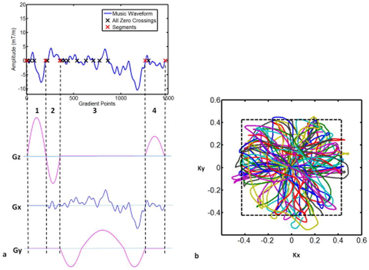
The music waveform was first preprocessed. (a) zero crossings of the preprocessed waveform were located (black crossings). Depending on the requirement of the minimum RF duration and acquisition time, the zero crossings were grouped such that each TR had four music segments (red crossings). The first segment (1) was used to design slice selection gradient. The second segment (2) was used to design slice selection dephasing gradient. The third segment (3) was used to design readout gradient, and the fourth segment (4) was used to design spoiling gradient. Music segments with total areas of zero were played in Gx in segment (2) and (4). (b) k-space trajectories derived from the 2D gradients from (a). K_x (1/milliseconds), K_y (1/milliseconds)

While one could potentially solve for an ideal set of gradient waveforms at every point in the sequence as in (15), we have observed that one can maintain the sound quality while making relatively significant deviations from the actual music waveform as long as the basic timing of the music is preserved. Thus one can use relatively simplistic gradient waveforms to achieve all of the goals set out above. Since the duration of the slice selection and slice selection dephasing/spoiling gradients were relatively short and the zero crossings of the music were preserved, the gradients from the slice selection and spoiling/rephasing sections in each TR were directly replaced by scaled half-sine waveforms. Since the timing is fixed, the peak amplitude is given by:

$$G_{s\_i}=G_{\mathit{sine}\_i}\times \frac{M_i}{\sum G_{\mathit{sine}\_i}}$$ [1]

where i is the index of the segments, G_{sine_i} = sin(t_i/N_si × π), i =1, 2 and 4, N_s1, N_s2 and N_s4 are the number of points in segment 1, 2 and 4, respectively, t_i is from 1 to N_si. M_i is the required gradient area for each segment. The gradient area of the M₁ (slice selection) and M₂ (slice selection dephasing) are determined by RF duration, time bandwidth product and slice thickness, and M₄ is the gradient area for a specific rephasing (for bSSFP-based sequence) or spoiling moment (for nbSSFP-based sequence). In this study, in addition to the spoiling moment introduced from the slice selection and slice selection dephasing gradients, a 2π per voxel dephasing was added at the end of each TR. Introducing this constant dephasing moment minimized B₀ effects(16,17) in contrast to the fully balanced gradients used in the original MRF acquisition. For the RF excitation, VERSE RF pulses(18,19) were used to match the G_{s_1} music waveform and to achieve the same slice profile from a sinc pulse with a duration of 2000 us and a time bandwidth product of 8, such that the excitation profile is maintained independent of the TR.

While there are infinite possibilities, the gradients from the third segment, which is where the signal is read out, were designed according to two constraints: 1) These gradients must start and end at zero and 2) they must have a total gradient area of zero. This process begins by directly using the music waveform for these gradients. In this case, the first constraint is already achieved by determining the segment length based on the zero crossings. An efficient way to correct the gradient area was to subtract an additional gradient in the shape of a half sine wave:

$$G_x=s-G_{\mathit{sine}}\times \frac{\sum S}{\sum G_{\mathit{sine}}}$$ [2]

where G_x is the target gradient and s is the music waveform. In this way, the area of the gradient was scaled while the zero crossings at two ends of the gradient were preserved. Any gradient shape that preserves the end points could be used here. As shown below, this small, smooth additional waveform had a negligible effect on the sound of the acquisition.

At this point, the sequence would only read out a single line that could be rotated from TR to TR similar to a radial scan. However in this case, there are infinite choices for encoding a second dimension of the acquisition. Again, it was found that the addition of relatively simple waveforms was able to preserve the sound while improving the encoding efficiency. In this study, a three-lobed balanced waveform was added in the orthogonal direction to the music waveform to increase the k-space coverage. The resulting k-space sampling pattern is shown in Figure 1b. Although these additional gradients contribute to the sound, the amplitudes and slew rates of these gradients are generally lower than that of the music-based gradients, and thus the added sound volume is also low. During the acquisition, both gradient waveforms were rotated by 0.9 degrees from one TR to the next, so that each TR along the signal evolution had different spatial encoding without dramatically altering the music sound. The k-space trajectories from 100 TRs are shown in Figure 1b, where each color represents the music-based trajectory from one individual TR. Since the desired image resolution was lower than the maximal extent of the k-space samples, only the inner range of k-space samples was selected and used for image reconstruction.

A similar approach to sequence design was used to design a 3D slab selective sequence. In this case, the slice direction was encoded through conventional Fourier encoding where each partition was acquired through a separate repetition of the 2D music sequence described above, with an additional half-sine gradient added to the slice rephaser (the second segment in Figure 1) for conventional phase encoding.

As a final option, we investigated a fully non-selective 3D encoded sequence. As shown in Figure 2, there were only two music segments required: RF excitation and balanced readout gradients. In this case, no gradients were applied during the short RF pulse interval. Following this, a bSSFP readout with the gradient integral of zero from all three encoding directions was used to acquire the data. In this case the RF excitation could be kept very short such that it was largely outside of the audible range, thus very closely preserving the sound of this sequence. The music gradients were designed to be uniformly distributed on the sphere (20). While this results in a nearly isotropic spatial resolution, this encoding pattern requires significantly longer to fully sample k-space, and we only demonstrate undersampled variants here.

Figure 2. Diagram of the music conversion for a 3D non-selective MRF-Music sequence.

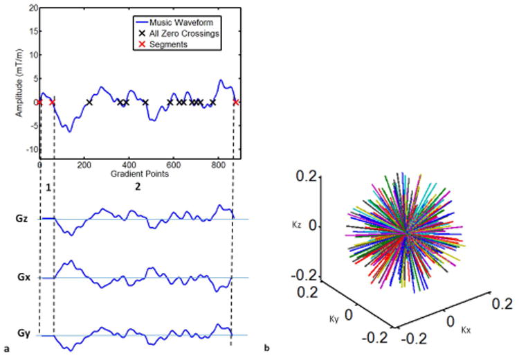
The zero crossings of the music waveform were grouped such that each TR had two music segments (red crossings). No gradients were applied during the short RF pulse interval (1). The second segment (2) was used to design a bSSFP readout with the gradient integral of zero from all three encoding directions. (b) 3D radial k-space trajectories derived from the 3D gradients from (a). K_x (1/milliseconds), K_y (1/milliseconds) and K_z (1/milliseconds).

Methods

MRF-Music Sequence Design

The music gradients were implemented with a variable FA and TR pattern (Fig. 3) in a 2D MRF-Music sequence. The conversion time from an mp3 music to the gradients used in a 2D MRF-Music sequence was 2 minutes on a desktop PC in Matlab (Natick, MA, USA). Even though the exact flip angle series was arbitrary, the MRF-Music sequence used here was designed based on the original MRF sequence. The sequence used a series of repeating sinusoidal curves with a period of 250 TRs and alternating maximum flip angles. In the odd periods, the flip angle was calculated as FA_t= 10 + sin(2πt/500) × 50 + random, where t is from 1 to 250, random(5) is a function to generate uniformly distributed values with a range of 0-5. In the even periods, the previous period's flip angle was divided by 2 to add some additional signal variations among different sections. The sinusoid shape allows the signal to build up by using slowly increased flip angles. A 50 TR gap with no flip angle between sections was chosen because this gave time for the magnetization to relax, in order to keep relatively high signal intensity. The signal evolution during this period also shows a nearly pure T₂ relaxation as well. In addition, adiabatic inversion pulses were added in every 1200 TRs to improve T₁ sensitivity. The RF phases were set to 0 at all TRs.

Figure 3. 2D MRF-Music sequence pattern.

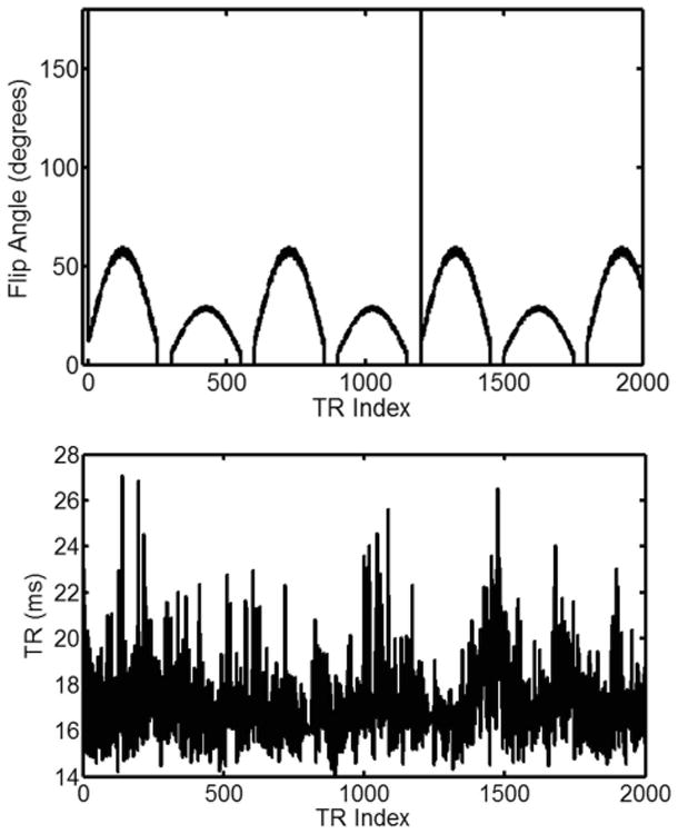
The first 2000 points of flip angle (FA) and repetition time (TR) pattern that were used in this study. 8.67 cm × 9.5 cm, 600 DPI

Acquisition

All data were acquired on a 3T whole body scanner (Siemens Skyra, Siemens Healthcare, Erlangen, Germany) with a 16-channel head receiver coil (Siemens Healthcare, Erlangen, Germany). The range of the k-space samples that were used in the reconstruction was determined by the desired image resolution. The 2D MRF-Music acquisition used a square field of view (FOV) of 300 × 300 mm² and a resolution of 1.2×1.2 mm². Images were acquired at the iso-center. The slice thickness was 5 mm. A total acquisition time of 68 seconds, corresponding to 4000 time points, was used for the 2D acquisitions. For the 3D slab selective MRF-Music acquisition, 4000 time points were acquired at each of 16 partitions, resulting in a total acquisition of 18.4 minutes. The FOV was 300×300×48 mm³ with a resolution of 1.2×1.2×3 mm³. For the 3D non-selective MRF-Music, 1579 time points were acquired with 144 repetitions for a total acquisition time of 37 minutes. The FOV was 300×300×300 mm³ with an isotropic resolution of 2.3×2.3×2.3 mm³. Images from each time point were reconstructed separately using multi-scale iterative reconstruction described briefly below and in (21). The resultant time series of images were used to determine the value for the parameters (T₁, T₂, and M₀) as in the original MRF method. In this study, the minimum RF duration was 2000 us for the 2D MRF-Music sequence and 3D slab-selective sequence, and 250 us for the 3D non-selective sequence. The minimum sampling time per TR was 8000 us.

All in vivo experiments were performed under the IRB guidelines, including written informed consent. A MRF sequence as described in(14) with a single-shot spiral trajectory was used to quantify T₁, T₂ and M₀ at the same location as a comparison. In a phantom study, ten cylindrical phantoms were constructed with varying concentrations of Gadopentetate dimeglumine (Magnevist) and agarose (Sigma) to yield different T₁ and T₂ values ranging from 200 to 1534 ms and 30 to 133 ms, respectively. The standard T₁ method, used for comparison was the inversion recovery spin echo (SE) sequence (8 TIs 21-3500 ms with a TE of 12 ms and a TR of 10 seconds). The standard T₂ method was a repeated spin echo sequences with TEs = [13 33 63 93 113 153 203] ms, TR of 10000 ms and total acquisition time of 52 minutes. T₁ values were calculated pixel-wisely by solving the equation S(TI) = a + bexp(−TI/T1) using a three-parameter nonlinear least squares fitting routine. T₂ values were determined pixel-wisely by solve the equation S(TE) = aexp (−TE/T2) using a two-parameter nonlinear least squares fitting routine.

Dictionary Design

The dictionary used in the matching algorithm was simulated using the extended phase graph formalism(22) and implemented in MATLAB (The MathWorks, Natick, MA). Signal time courses with different sets of characteristic parameters (T₁ and T₂) were simulated. The ranges of T₁ and T₂ for the in vivo study were chosen according to the typical physiological limits of tissues in the brain: T₁ values were taken to be between 100 and 5000 ms (in an increments of 10 ms below a T₁ of 1000 ms, an increment of 20 ms between 1000 ms and 2000 ms and in an increment of 300 ms above.) The T₂ values included the range between 20 and 3000 ms (with an increment of 5 ms below a T₂ of 100 ms, an increment of 10 ms between 100 ms and 200 ms and an increment of 200 ms above a T₂ of 200 ms.). In each TR, the effects of RF excitation, T₁ and T₂ relaxation in varying TR and dephasing from the spoiling gradient in the slice selection direction were simulated. Because the total dephasing moment in each TR was constant and larger than 2π, the number of states was assumed to advance once after each TR. A total of 4539 dictionary entries, each with 4000 time points, were generated in 18 minutes on a standard desktop computer.

Multi-scale Iterative Methods

Since the MRF-Music acquisition is highly undersampled (1/400^th for the image resolution of 1.2×1.2 mm²), directly pattern matching based on (23) would introduce artifacts in T₁ and T₂ maps. Therefore, a multi-scale iterative method (21) was used to iteratively improve the quality of the maps. The multi-scale iterative method was initiated by reconstructing the MRF image series at a very low spatial resolution, for example, one-quarter of the original resolution using non-uniform Fourier transform (NUFFT)(24). Images were reconstructed from each individual coil and then combined using the adaptive coil combination method (25). In the pattern matching step, one dictionary entry was selected for each measured pixel location using template matching. In this case, the vector dot-product was calculated between the measured time course and all dictionary entries (appropriately normalized to each having the same sum squared magnitude) using the complex data for both. The dictionary entry with the highest dot-product was then selected as most likely to represent the true signal evolution. The proton density (M₀) of each pixel was calculated as the scaling factor between the measured signal and the simulated time course from the dictionary. These quantitative maps had low resolution but with relatively fewer artifacts from the undersampled measurement. In the following iteration, a new set of signal evolutions were simulated from the current maps. The method then enforced fidelity of the newly simulated data to the acquired data at slightly higher spatial resolution by replacing the originally sampled data in the k-space. When convergence was reached, parameter maps were obtained through template matching of the final image series.

Preparation of the Supporting Audio Files

The six supplemental audio files were recorded using Zoom H2n Handy Recorder (Zoom). The recorder was placed on the stationary patient table, which is about 2 meters away from the center of the MR scanner. Additionally, a piece of foam cushioned the recorder from direct contact to the platform to isolate the recorder from direct table vibration. In each recording, 5 seconds of ambient noise from the room (when no scan was performed) was recorded, followed by 30 seconds of the sound from one acquisition, which is then followed by another 5 seconds of the ambient noise. The sound levels were adjusted to prevent clipping of the audio waveforms and were maintained at a constant level for all recordings.

Comfort Level Survey

To evaluate the comfort level of the MRF-Music acquisition compared to a conventional MRI acquisition, 10 volunteers who had never had any previous MRI scan (4 women and 6 men, aged between 20 and 29) were scanned by four different acquisitions. These included two conventional acquisitions, a conventional turbo spin echo (TSE) and a conventional diffusion-weighted EPI. Both are key components of every MRI exam of the head. In particular the EPI scan was chosen to represent a worst-case of acoustic noise. A 2D MRF-Music acquisition was performed as described in the methods section. A final control acquisition was performed wherein no gradient switching occurred; the volunteer could only hear the ambient noise from the room. All volunteers were given earplugs for MR standard ear protection. The instructions given to the subject are included in the supporting material. In short, the volunteers were asked to rate their comfort level immediately after a one-minute acquisition with a self-selected scaling from 1-10 (1=most uncomfortable and 10=most comfortable) for each of four different acquisitions, presented in random order with 3 repetitions.

Statistical Analysis

Quantitative estimation of the accuracies and efficiencies of MRF-Music and MRF were calculated pixel-wise using a bootstrapped Monte Carlo method as in Riffe et al (26). Two sets of data were acquired for each scan: the encoded signal acquired as described in the ‘Acquisition’ section, and the noise signal acquired using the same sequence but with all FA as 0. Fifty reconstructions were then calculated by randomly permuting the noise signal and adding them to the encoded signal before reconstruction and quantification. The means and standard deviations of T₁ and T₂ along 50 repetitions within a square region of interest for each phantom were calculated. Afterwards, the efficiency of the methods was calculated as (27):

$$\mathit{\text{Efficiency}}=T_{n}NR/\sqrt{T_{\mathit{\text{seq}}}},n=1,2$$ [4]

where T_nNR is the T₁ or T₂ to noise ratio (defined as the T₁ or T₂ value divided by the standard deviation). T_seq is the total acquisition time.

The concordance correlation coefficients(28) (ρ_c) were calculated as:

$${\rho }_c=\frac{2S_{12}}{S_1^2+S_2^2+{({\overline{Y}}_2-{\overline{Y}}_1)}^2}$$ [5]

where Y₁ and Y₂ denotes the T₁ or T₂ values from two different methods, n is the number of phantoms,

$$Y_j=({\sum }_{i=1}^n{Y}_{ij})/n,S_j^2=({\sum }_{i=1}^n{(Y_{ij}-{\overline{Y}}_J)}^2)/n,j=1,2\text{and}{S}_{12}=({\sum }_{i=1}^n(Y_{i1}-{\overline{Y}}_1)(Y_{i2}-{\overline{Y}}_2))/n.$$

The survey data contained the scores from 10 volunteers as a pilot study, with each volunteer rating their perceived comfort level from 12 different exams which consisted of three repetitions of four different acquisition protocols in a randomized order using a random number generator. First, the average score of the 3 replicates from each volunteer and each protocol was calculated, resulting in total of 40 observations (10 volunteers × 4 observations). These data were analyzed using a two-sided randomized block analysis of variance (ANOVA), with subjects as blocks and protocols as treatments. The normality assumption was checked in the ANOVA both graphically and also using the Shapire-Wilk test on the residuals. The Shapiro-Wilk p-value of 0.63 indicated that there was no evidence of non-normality. Based on the ANOVA, pairwise comparisons of means of the four treatments were made, using a Bonferroni multiple comparison correction to control familywise type 1 error rate.

Results

Comfort Level of MRF-Music

Phantom and in vivo studies were performed in both 2D and 3D MRF-Music acquisitions to quantify T₁, T₂ and proton density (M₀) maps simultaneously. The included Supplemental Audio Files demonstrate the various sounds generated by the different acquisitions tested here. All are recorded at the same gain level, and thus these files should be directly comparable to the sound level in the room. Supplemental Audio Files 1 and 2 demonstrate the sounds generated by two kinds of MRI acquisitions used in many standard exams. The first is a turbo spin echo sequence (TSE), while the second is an echoplanar acquisition (EPI). Both of these acquisitions demonstrate the conventional banging sound associated with MRI. Supplemental Audio File 3 demonstrates the sound generated by a standard MRF scan (Fig. 1d of reference(14)). Because the MRF sequence was designed to have a high sampling efficiency by working near the hardware limits of the scanner using pseudorandom switching patterns, the sound of the MRF sequence was much louder than majority of the conventional MRI scans.

Supplemental Audio File 4 represents the sound generated by the 2D version of MRF-Music based on a recording of Yo Yo Ma playing Bach's Cello Suite 1 for a total acquisition time of 68 seconds. The underlying music sound is clearly evident, although some additional distortions can be heard due to the required slice selection gradient switching.

Supplemental Audio File 5 represents the sound generated by the 3D, slab selective version of MRF-Music. This 3D MRF-Music acquisition took about 18.4 minutes to quantify T₁, T₂ and M₀ values of tissues in a larger imaging volume of 16 imaging slice partitions. The audio quality of this acquisition was further improved due to the lower switching requirements for the larger excited slice in the 3D acquisition. Supplemental Audio file 6 represents the sound generated by the 3D, non-selective version of MRF-Music, which took about 37 minutes to quantify an isotropic 3D volume of 300×300×300 mm³. Because there was no slice selection gradient switching, the 3D non-selective version of MRF-Music generated the best sound in comparison to the 2D and 3D slab selective versions. In both of the 3D cases, a segment of the audio is repeated multiple times.

All the scores from the survey were used for the statistical analysis with no exclusion. The result of the pairwise comparisons of the mean scores in the ANOVA showed a significant improvement of the MRF-Music in terms of the comfort level in comparison to both EPI and TSE sequences (Bonferroni-adjusted P<0.001), with an average scores (± SD) of 7.2±1.2 from MRF Music and 4.5±1.4 and 4.9±1.5 from EPI and TSE, respectively. The control had the highest average score of 9.4±0.9.

Accuracy and Efficiency of MRF-Music

The T₁ and T₂ values of the phantom study from a 2D MRF-Music scan were compared with those from the conventional MRF and the standard quantitative methods (Fig. 4a and 4b). The concordance correlation coefficient (CCC) for T₁ and T₂ between MRF-Music and the standard MRI-based measurements were 0.9931 and 0.9897, respectively. The CCC for T₁ and T₂ between MRF and the standard measurements were 0.9981 and 0.9929, respectively. The CCC indicated that both methods were in good agreement with the conventional MRI methods. The theoretical comparison of the efficiency between MRF and MRF-Music was calculated as the precision in T₁ or T₂ per square root of imaging time. As shown in Figure 4c and 4d, MRF outperformed MRF-Music by an average factor of 1.11 and 1.32 for T₁ and T₂ respectively For example, at a T₁ of 1155 ms, MRF showed an efficiency of 16.93 while the MRF-Music showed an efficiency of 14.50. However, even though the MRF-Music efficiency is lower than MRF, it is still more than adequate for most clinical questions. For example, the phantom with a T₁ value of 1155 ms had a precision of ±10.90ms and ±9.67 ms with a 68-second scan, respectively for MRF and MRF-Music. Therefore, both methods achieved high precision in a short acquisition time.

Figure 4. Accuracy and efficiency of the 2D MRF-Music scan.

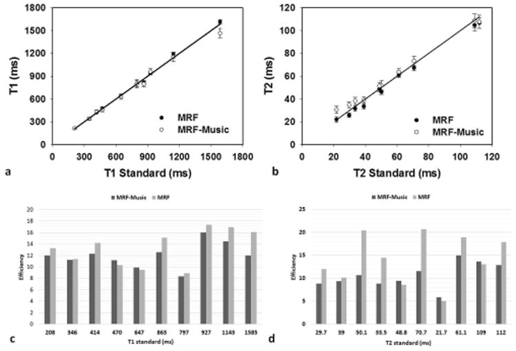
(a), (b), The T₁ and T₂ values obtained from the 2D MRF-Music scan from 10 phantoms were compared with the values acquired from the MRF and the standard measurements. (c),(d), The efficiency of T₁ and T₂ obtained from MRF-Music were compared to those from MRF. (a) and (b) show mean+/− s.d. of the results over a 25-pixel region in the center of each phantom. 8.67 cm × 6.13 cm, 600DPI

For the in vivo study, an example of a reconstructed image from 2D MRF-Music scan along with the signal evolution from one of the imaging pixels are shown in Figure 5. Due to the factor of 400 undersampling rate and randomized acquisition patterns, images reconstructed from the acquired data were corrupted by aliasing errors. Because these errors were incoherent with the expected signal, most of the errors do not affect the subsequence processing used in the estimation of quantitative MR parameters. Figure 5c and 5e show the T₁ and T₂ maps obtained from direct template matching without using the multi-scale iterative method, as described in (14). Some residual aliasing artifacts can be seen in both maps. Figure 5d and f are the maps obtained using the multi-scale iterative method. After 4 iterations, the image quality from both maps are improved. The T₁, T₂ and M₀ maps were then compared to those acquired at the same slice position from a MRF scan in Figure 6. Both quantitative values and tissue appearance of the T₁ and T₂ maps are in good agreement. A minor difference can be seen on the anterior region of the head, where a signal drop can be seen in the sinuses, making it difficult to retrieve the T₁ and T₂ values in this region. White matter (WM) and gray matter (GM) regions were then selected from the resultant maps from the MRF-Music acquisition. The mean T₁ and T₂ values obtained from each region were shown in Table 1. Figure 7 show the T₁ and T₂ maps obtained from a patient with brain tumor (Figure 7a,b) and a patient with pituitary tumor (Figure 7e,f). The corresponding T₁ and T₂ weighted images as shown in Figure 7c,d and Figure 7g,h were calculated based on these maps using the TI of 500 ms and TE of 60 ms, respectively.

Figure 5. In vivo results of the 2D MRF-Music scan.

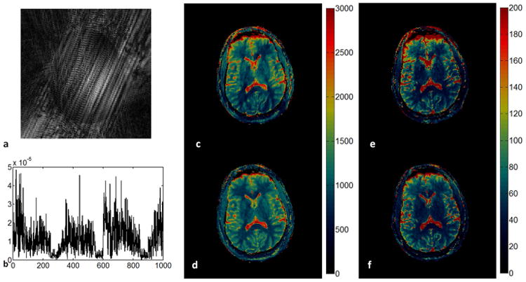
(a). An image at the 11^th repetition time out of 4000 was reconstructed from only one music trajectory demonstrating the significant errors from undersampling. (b). one example of the acquired signal evolution from the first 1000 time points. (c) and (d): T1 map generated without and with the multi-scale iterative method. (e) and (f): T2 map generated without and with the multi-scale iterative method. 13.02 cm × 7.1 cm, 600 DPI

Figure 6. Comparison of the maps obtained from MRF-Music and MRF scans.

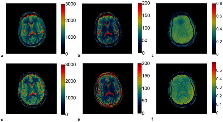
(a)-(c), T₁(a), T₂ (b) and proton density (c) maps obtained from the MRF-Music sequence. (d)-(f), T₁(d), T₂(e) and proton density (f) maps obtained from the original MRF sequence. T₁ (color scale, milliseconds), T₂ (color scale, milliseconds) and M₀ (normalized color scale). 13.02 cm × 7.3cm, 600 DPI

Table 1.

In vivo T₁ and T₂ relaxation times obtained from 2D MRF-Music at 3T, and the corresponding values reported in the literatures. The values were from the mean±s.d. of the results over 20-pixel ROIs.

	T1 (ms)	T2 (ms)
White Matter (this work)	847 ± 49.21	48 ± 6.32
White Matter (previously reported)	788∼898	63∼80
Gray Matter (this work)	1223 ± 65.11	64.31±5.23
Gray Matter (previously reported)	1286∼1393	78∼117

Figure 7. In vivo results of the patient scans.

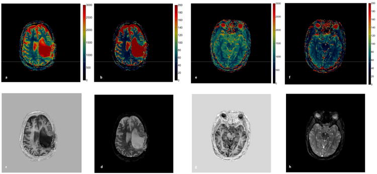
(a and b) T1 and T2 maps were generated from a 2D MRF-Music scan of a brain tumor patient. (e and f) T1 and T2 maps were from a patient with pituitary tumor. (c and g) the corresponding T1-weighted images were calculated from the T1 map with TI of 500 ms. (d and h) T2-weighted image were calculated from the T2 map with a TE of 60 ms. 17.56 cm × 8.1cm, 600 DPI

For the 3D slab selective MRF-Music scan, T₁, T₂ and M₀ maps from 16 slice partitions were acquired from a single acquisition to cover a 300×300×48 mm³ field of view with the image resolution of 1.2×1.2×3 mm³. Figure 8 shows the T₁ and T₂ maps from the 7^th to 10^th partitions, which demonstrate comparable image quality as the maps from the 2D MRF-Music scan, with a few grainy appearing artifacts in the T₂ maps.. The 3D non-selective MRF-Music scan achieved the best volume coverage and through plane resolution. Transversal, sagittal and coronal views of the 3D volumes of 300×300×300 mm³ can be visualized with an isotropic resolution of 2.3×2.3×2.3 mm³ (Fig. 9). The off-resonance maps were obtained in addition to the T₁, T₂ and M₀ maps in this version, because the slice selection gradient was fully balanced, as in the original MRF acquisitions. Some residual aliasing artifacts, which appear as stripe-like artifacts, can be seen in sagittal and coronal views.

Figure 8. In vivo results of the 3D slab selective MRF-Music scan.

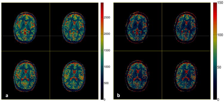
T₁ maps (a), T₂ maps (b) from the 7^th to 10^th out of 16 partitions were obtained from a single MRF-Music scan. T₁ (color scale, milliseconds) and T₂ (color scale, milliseconds). 17.56 cm × 8.12 cm, 600DPI

Figure 9. In vivo results of the 3D non-selective MRF-Music scan.

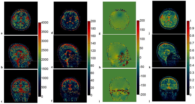
T₁ maps (a-c), T₂ maps (d-f), off-resonance maps (g-i) and M₀ maps (j-l) were shown in the axial, sagittal and coronal views, respectively. T₁ (color scale, milliseconds), T₂ (color scale, milliseconds), off-resonance (color scale, Hertz) and M₀ (normalized color scale). 17.56 cm × 9.68 cm, 600 DPI

Discussion

MRF-Music is an application of the MRF concept for the purpose of increasing patients' comfort in a fully quantitative MR exam. In this study, it was demonstrated that MRF-Music can combine data acquisition with the sound of a musical performance to quantify multiple key parameters of the tissues, such as T₁, T₂ and M₀, in a clinically acceptable time.

In the phantom study, as shown by the high value of the concordance correlation coefficients, both T₁ and T₂ values from the MRF-Music were in agreement with those from the standard measurement. T₂ values below 35 ms were overestimated from the MRF-Music scan, which might be due to the relatively long TR (average of 17 ms) of the sequence. MRF-Music also provided in vivo maps with image resolution of 1.2×1.2 mm², which is equivalent to our conventional clinical scans. The difference in the proton density maps between MRF-Music and MRF in Figure 6 was probably due to different receiver sensitivity profile. As compared to the previously reported literature values(29,30) in Table 1, the T₂ values from the MRF-Music scan were relatively lower. In this study, initial implementation and results from a 3D non-selective MRF-Music were presented. Because of the high undersampling ratio and the additional parameter that needs to be quantified, the current version of the 3D non-selective MRF-Music scan provided maps with residual aliasing artifacts. As shown in Figure 9, the aliasing artifacts, which appear as striping artifacts, are mainly seen in the sagittal and coronal views. This is likely due to insufficient sampling density along z-x and z-y directions. These artifacts could be potentially resolved by iteratively designing the acquisition trajectory based on the music waveforms and/or acquiring more repetitions

Within this framework, there is no restriction on the choice of the music waveform. Different music selections may alter the scan efficiency, but after pre-processing, such as audio compression, and proper post-processing, such as gradient and RF pulse design, any music can be used in the MRF-Music scan. Therefore, except for designing some of the MRF-specific acquisition parameters, such as the flip angle series and the specific slice profile waveforms, any music or any sound effect could be flexibly incorporated into the sequence design. In addition, the conversion time to generate all gradients from the music is only 2 minutes, which is fast enough to generate the music scan based upon the patients' choice before their scan.

The VERSE pulse is sensitive to the off-center shift. In the current implementation, the RF pulses for the 2D MRF-Music acquisition were designed with relatively short duration (approximately 2000us) and with low flip angles (with the maximum of 60 degrees and average of 25.5 degrees). Because the slice profile of the VERSE pulse was designed based on a sinc pulse with a duration of 2000 us and a time bandwidth product of 8, there is also no slice profile issue relating with the RF pulse. Further optimization of the slice selection gradients and VERSE pulse will be investigated to improve the image quality in the presence of the off-resonance along the slice selection direction. These issues were reduced in the 3D slab case, since one has more freedom in positioning the slice at isocenter while maintaining full coverage of the anatomy of interest. Although the unbalanced gradient moment introduced from the nbSSFP-based sequence alleviates the banding artifacts from the bSSFP-based sequence, it also makes the sequence potentially sensitive to flow and motion along the unbalanced gradient direction (31). However, the incoherent sampling from music trajectories as well as the pattern recognition basis of MRF have been shown to provide good motion tolerance. The signal changes introduced from flow are uncorrelated with the signal evolution from other tissue types, and are largely ignored from the pattern recognition process of the MRF(14,32).

Because the focus of this study was on the production of high quality sound from the scanner, the sampling efficiency of the MRF-Music sequence was not as high as the original MRF, and was clearly not optimized to a final form. Optimization methods can be used in the future to improve the audio performance and sampling efficiency with the hope that the efficiency of the MRF-Music sequence is mostly independent of the choice of the music. However, since MRF-Music shares many of the same features of MRF, namely that the signal never settles into a steady state, the continuous oscillatory signal allows one to acquire more informative data by acquiring over a longer time. Thus one could adjust the time of the acquisition to compensate for any change in efficiency. Even still, the current 2D MRF-Music quantifies parameters at clinically acceptable accuracy and precision using only less than one fourth of a complete classical piece of music. The acquisition speed can be further accelerated by applying parallel imaging techniques(33–35)and compressed sensing(36–39) in the spatial domain, neither of which were included here. Although there are still artifacts on the maps from the 3D non-selective MRF-Music sequence, this sequence type is promising because it not only achieves better spatial coverage and higher through plane resolution, but also provides the best sound quality compared to the sequences that requires slice selective gradient design. In addition, 3D trajectories allow one to achieve higher acceleration rate. Currently, the 3D non-selective MRF-Music acquisition requires 37 minutes to obtain 3D maps from four parameters. Further optimization of the music gradients and trajectory segmentation will potentially accelerate the acquisition and improve the image quality.

Thus we believe that MRF-Music represents a broadly applicable, flexible framework to improve patient care in MRI.

Supplementary Material

Supp AudioS1

Supporting Audio File 1: This audio demonstrates the sound generated from a turbo spin echo sequence (TSE), which is one of the most common MRI exams of the head. (audio format : .mp3 829kB)

Supporting Audio File 2: This audio demonstrates the sound recorded from an echo-planer imaging sequence (EPI), which is also a key component of every MRI exam of the head. The EPI scan is chosen to represent a worst-case of acoustic noise in the MR scan. (audio format : .mp3 900kB)

Supporting Audio File 3: This audio demonstrates the sound generated by a standard MRF scan. The sound is much louder than that from the conventional MRI exams. (audio format : .mp3 920kB)

Supporting Audio File 4: This audio demonstrates the sound generated by the 2D version of MRF-Music based on a recording of Yo Yo Ma playing Bach's Cello Suite No.1. The underlying music sound is evident, except for a few distortions due to the required slice selection gradient switching. (audio format : .mp3 863kB)

Supporting Audio File 5: This audio demonstrates the sound generated by the 3D slab selective version of MRF-Music based on a recording of Yo Yo Ma playing Bach's Cello Suite No.1. The music sound distortion is reduced due to the lower switching gradients. (audio format : .mp3 906kB)

Supporting Audio File 6: This audio demonstrates the sound generated by the 3D non selective version of MRF-Music based on a recording of Yo Yo Ma playing Bach's Cello Suite No.1. Because there is no slice selection gradient switching, 3D non-selective MRF-Music generates the best sound in comparison to the 2D and 3D slab selective versions. (audio format : .mp3 1006kB)

Supporting Note: Instructions given to each subject prior to study of the comfort level:

We are going to be placing you in an MRI scanner. As you may know, an MRI scanner makes noise while we are taking an image. I am going to be using several different ways of taking an image and would like you to tell me how they make you feel. After each image, I will ask you to rate your comfort level on a scale of 1 to 10. 1 will indicate that you are very uncomfortable, while 10 indicates that you are very comfortable. Use your individual judgment in setting the scores for each scan that I ask you to rate.

Could you please give me your score from 1 to 10?

References

- 1.McJury M, Shellock FG. Auditory Noise Associated With MR Procedures: A Review. J Magn Reson Imaging. 2000;12:37–45. doi: 10.1002/1522-2586(200007)12:1<37::aid-jmri5>3.0.co;2-i. Internet. [DOI] [PubMed] [Google Scholar]
- 2.Brummett RE, Talbot JM, Charuhas P. Potential Hearing Loss Resulting From MR Imaging. Radiology. 1988;169:539–40. doi: 10.1148/radiology.169.2.3175004. Internet. [DOI] [PubMed] [Google Scholar]
- 3.Quirk ME, Letendre AJ, Ciottone RA, Lingley JF. Anxiety in Patients Undergoing MR Imaging. Radiology. 1989;170:463–6. doi: 10.1148/radiology.170.2.2911670. Internet. [DOI] [PubMed] [Google Scholar]
- 4.Kanal E, Shellock FG, Talagala L. Safety Considerations in MR Imaging. Radiology. 1990;176:593–606. doi: 10.1148/radiology.176.3.2202008. Internet. [DOI] [PubMed] [Google Scholar]
- 5.Philbin MK, Taber KH, Hayman LA. Preliminary Report: Changes in Vital Signs of Term Newborns During MR. Am J Neuroradiol. 1996;17:1033–6. Internet. [PMC free article] [PubMed] [Google Scholar]
- 6.Amaro E, Williams SCR, Shergill SS, Fu CHY, MacSweeney M, Picchioni MM, Brammer MJ, McGuire PK. Acoustic Noise and Functional Magnetic Resonance Imaging: Current Strategies and Future Prospects. J Magn Reson Imaging. 2002;16:497–510. doi: 10.1002/jmri.10186. Internet. [DOI] [PubMed] [Google Scholar]
- 7.Bandettini PA, Jesmanowicz A, Van Kylen J, Birn RM, Hyde JS. Functional MRI of Brain Activation Induced by Scanner Acoustic Noise. Magn Reson Med. 1998;39:410–6. doi: 10.1002/mrm.1910390311. Internet. [DOI] [PubMed] [Google Scholar]
- 8.Chen CK, Chiueh TD, Chen JH. Active Cancellation System of Acoustic Noise in MR Imaging. IEEE Trans Biomed Eng. 1999;46:186–91. doi: 10.1109/10.740881. Internet. [DOI] [PubMed] [Google Scholar]
- 9.Mansfield P, Glover P, Bowtell R. Active Acoustic Screening: Design Principles for Quiet Gradient Coils in MRI. Meas. Sci Technol. 1994;5:1021–1025. [Google Scholar]
- 10.Bowtell RW, Mansfield P. Quiet Transverse Gradient Coils: Lorentz Force Balanced Designs Using Geometrical Similitude. Magn Reson Med. 1995;34:494–497. doi: 10.1002/mrm.1910340331. Internet. [DOI] [PubMed] [Google Scholar]
- 11.Counter SA, Olofsson A, Grahn EEHF, Borg E. MRI Acoustic Noise : Sound Pressure and Frequency Analysis. J Magn Reson Imaging. 1997;7:606–611. doi: 10.1002/jmri.1880070327. [DOI] [PubMed] [Google Scholar]
- 12.Pierre EY, Grodzki D, Aandal G, Heismann B, Badve C, Gulani V, Sunshine JL, Schluchter M, Liu K, Griswold Ma. Parallel Imaging-Based Reduction of Acoustic Noise for Clinical Magnetic Resonance Imaging. Invest Radiol. 2014;49:620–6. doi: 10.1097/RLI.0000000000000062. Internet. [DOI] [PubMed] [Google Scholar]
- 13.Loeffler R, Hillenbrand C. Anxiety Loss Offered by Harmonic Acquisition (ALOHA) Proceedings 10th Scientific Meeting, International Society for Magnetic Resonance in Medicine. 2002;10 [Google Scholar]
- 14.Ma D, Gulani V, Seiberlich N, Liu K, Sunshine JL, Duerk JL, Griswold MA. Magnetic Resonance Fingerprinting. Nature. 2013;495:187–192. doi: 10.1038/nature11971. Internet. [DOI] [PMC free article] [PubMed] [Google Scholar]
- 15.Ma D, Gulani V, Griswold MA. Using Gradient Waveforms Derived from Music in MR Fingerprinting (MRF) to Increase Patient Comfort in MRI. Proceedings 22th Scientific Meeting, International Society for Magnetic Resonance in Medicine. 2014:26. [Google Scholar]
- 16.Gyngell ML. The application of steady-state free precession in rapid 2DFT NMR imaging: FAST and CE-FAST sequences. Magn Reson Imaging. 6:415–9. doi: 10.1016/0730-725x(88)90478-x. Internet. [DOI] [PubMed] [Google Scholar]
- 17.Sekihara K. Steady-State Magnetizations in Rapid NMR Imaging Using Small Flip Angles and Short Repetition Intervals. IEEE Trans Med Imaging. 1987;6:157–164. doi: 10.1109/TMI.1987.4307816. [DOI] [PubMed] [Google Scholar]
- 18.Conolly S, Nishimura D, Macovski A. Variable-Rate Selective Excitation. J Magn Reson. 1988;78:440–458. [Google Scholar]
- 19.Pauly J, Nishimura D, Macovski A. A k-space analysis of small-tip-angle excitation. J Magn Reson. 1989;81:43–56. doi: 10.1016/j.jmr.2011.09.023. Internet. [DOI] [PubMed] [Google Scholar]
- 20.Saff E, Kuijlaars ABJ. Distributing Many Points on a Sphere. Math Intell. 1997;19:5–11. [Google Scholar]
- 21.Pierre E, Ma D, Chen Y, Badve C, Griswold M. Multiscale Reconstruction for Magnetic Resonance Fingerprinting. Proceedings 23rd Scientific Meeting, International Society for Magnetic Resonance in Medicine. 2015:0084. [Google Scholar]
- 22.Weigel M. Extended phase graphs: Dephasing, RF pulses, and echoes - pure and simple. J Magn Reson Imaging. 2014:00. doi: 10.1002/jmri.24619. Internet. [DOI] [PubMed] [Google Scholar]
- 23.Piccini D, Littmann A, Nielles-Vallespin S, Zenge MO. Spiral Phyllotaxis: The Natural Way to Construct a 3D Radial Trajectory in MRI. Magn Reso Med. 2011;66:1049–1056. doi: 10.1002/mrm.22898. Internet. [DOI] [PubMed] [Google Scholar]
- 24.Fessler JA, Sutton BP. Nonuniform Fast Fourier Transforms Using Min-Max Interpolation. IEEE Trans Signal Process. 2003;51:560–574. [Google Scholar]
- 25.Walsh DO, Gmitro AF, Marcellin MW. Adaptive Reconstruction of Phased Array MR Imagery. Magn Reson Med. 2000;43:682–90. doi: 10.1002/(sici)1522-2594(200005)43:5<682::aid-mrm10>3.0.co;2-g. Internet. [DOI] [PubMed] [Google Scholar]
- 26.Riffe MJ, Blaimer M, Barkauskas KJ, Duerk JL, Griswold MA. SNR Estimation in Fast Dynamic Imaging Using Bootstrapped Statistics. Proceedings 15th Scientific Meeting, International Society for Magnetic Resonance in Medicine. 2007;15:1879. [Google Scholar]
- 27.Deoni SCL, Rutt BK, Peters TM. Rapid Combined T1 and T2 Mapping Using Gradient Recalled Acquisition in the Steady State. Magn Reson Med. 2003;49:515–26. doi: 10.1002/mrm.10407. Internet. [DOI] [PubMed] [Google Scholar]
- 28.Lin LIK. A Concordance Correlation Coefficient to Evaluate Reproducibility. Biometrics. 1989;45:255–68. Internet. [PubMed] [Google Scholar]
- 29.Wansapura JP, Holland SK, Dunn RS, Ball WS. NMR Relaxation Times in the Human Brain at 3.0 Tesla. J Magn Reson Imaging. 1999;9:531–8. doi: 10.1002/(sici)1522-2586(199904)9:4<531::aid-jmri4>3.0.co;2-l. Internet. [DOI] [PubMed] [Google Scholar]
- 30.Hasan KM, Walimuni IS, Kramer La, Narayana Pa. Human brain iron mapping using atlas-based T2 relaxometry. Magn Reson Med. 2012;67:731–9. doi: 10.1002/mrm.23054. Internet. [DOI] [PMC free article] [PubMed] [Google Scholar]
- 31.Santini F, Bieri O, Scheffler K. Flow compensation in non-balanced SSFP. Proc 16th Sci Meet Int Soc Magn Reson Med. 2008 Internet. Toronto:3124. [Google Scholar]
- 32.Jiang Y, Ma D, Seiberlich N, Gulani V, Griswold Ma. MR fingerprinting using fast imaging with steady state precession (FISP) with spiral readout. Magn Reson Med. 2014:n/a–n/a. doi: 10.1002/mrm.25559. Internet. 00. [DOI] [PMC free article] [PubMed] [Google Scholar]
- 33.Griswold MA, Jakob PM, Heidemann RM, Nittka M, Jellus V, Wang J, Kiefer B, Haase A. Generalized Autocalibrating Partially Parallel Acquisitions (GRAPPA) Magn Reson Med. 2002;47:1202–10. doi: 10.1002/mrm.10171. Internet. [DOI] [PubMed] [Google Scholar]
- 34.Pruessmann KP, Weiger M, Börnert P, Boesiger P. Advances in Sensitivity Encoding With Arbitrary k-Space Trajectories. Magn Reson Med. 2001;46:638–51. doi: 10.1002/mrm.1241. Internet. [DOI] [PubMed] [Google Scholar]
- 35.Seiberlich N, Ehses P, Duerk J, Gilkeson R, Griswold MA. Improved Radial GRAPPA Calibration for Real-Time Free-Breathing Cardiac Imaging. Magn Reson Med. 2011;65:492–505. doi: 10.1002/mrm.22618. Internet. [DOI] [PMC free article] [PubMed] [Google Scholar]
- 36.Donoho DL. Compressed Sensing. IEEE Trans Inf Theory. 2006;52:1289–1306. [Google Scholar]
- 37.Candes EJ, Tao T. Near-Optimal Signal Recovery From Random Projections: Universal Encoding Strategies? IEEE Trans Inf Theory. 2006;52:5406–5425. doi: 10.1109/TIT.2006.885507. Internet. [DOI] [Google Scholar]
- 38.Lustig M, Donoho DL, Pauly JM. Sparse MRI: The Application of Compressed Sensing for Rapid MR Imaging. Magn Reson Med. 2007;58:1182–95. doi: 10.1002/mrm.21391. Internet. [DOI] [PubMed] [Google Scholar]
- 39.Bilgic B, Goyal VK, Adalsteinsson E. Multi-Contrast Reconstruction with Bayesian Compressed Sensing. Magn Reson Med. 2011;66:1601–15. doi: 10.1002/mrm.22956. Internet. [DOI] [PMC free article] [PubMed] [Google Scholar]
Associated Data
This section collects any data citations, data availability statements, or supplementary materials included in this article.
Supplementary Materials