Self-Guided Langevin Dynamics via Generalized Langevin Equation

Abstract

Self-guided Langevin dynamics (SGLD) is a molecular simulation method that enhances conformational search and sampling via acceleration of the low frequency motions of the system. This acceleration is produced via introduction of a guiding force which breaks down the detailed-balance property of the dynamics, implying that some reweighting is necessary to perform equilibrium sampling. Here we eliminate the need of reweighing and show that the NVT and NPT ensembles are sampled exactly by a new version of self-guided motion involving a generalized Langevin equation (GLE) in which the random force is modified so as to restore detailed-balance. Through the examples of alanine dipeptide and argon liquid, we show that this SGLD-GLE method has enhanced conformational sampling capabilities compared to regular Langevin dynamics (LD) while being of comparable computational complexity. In particular, SGLD-GLE is fully size extensive and can be used in arbitrarily large systems, making it an appealing alternative to LD.

Graphical Abstract

Introduction

Self-guided Langevin dynamics (SGLD)^1-3 was developed for efficient conformational exploration and sampling via selective acceleration of the low frequency modes of the molecules. SGLD is unique in that this acceleration is achieved without modifying the energy surface or raising temperature. SGLD has been applied to many studies of events arising on long time scales, such as the conformational reorganization of protein staphylococcal nuclease (SNase)⁴, hydration state and rotameric substates of SNase⁵, conformational transitions induced by dephosphorylation in nitrogen regulatory protein C (NtrC) protein⁶, conformational transitions in a membrane transporter protein lactose permease (LacY)⁷, and characteristics of the denatured state of the human prion (huPrP)⁸.

Because the guiding force involves a running average over the momentum at previous times, the detailed-balance property of the dynamics is broken in SGLD. In other words, SGLD is a non-equilibrium sampling method. This leads to a difficulty: the stationary distribution of the method, which has been termed the SGLD ensemble, is not known explicitly. In particular to perform canonical (NVT) or isothermal-isobaric (NPT) sampling via SGLD simulations requires reweighting².

The main result of the present work is to modify the SGLD equations of motion in a way that restores the detailed-balance property of the dynamics via a suitable modification of the random force. As we show below, this new SGLD-like equation is a generalized (non-Markovian) Langevin equation (GLE) which can be shown to samples exactly the NVT and NPT ensembles. This method, which we will refer to as SGLD-GLE, alleviates the need for reweighting and is therefore fully size extensive, as are molecular dynamics (MD) and Langevin dynamics (LD).

We note that the idea of using a GLE to selectively accelerate conformational exploration and sampling is not new: for example, it is at the core of the method of Ceriotti et al. ^{11, 12}. One contribution of the present work is to make the connection between these GLE-based methods and the general framework of SGLD, thereby allowing us to join forces and combine the expertise that has been built in both contexts. We expect that this strategy will be useful in a wide variety of contexts. In particular SGLD-GLE is more efficient than standard LD and with a comparable computational cost, making it an interesting alternative to it.

Theory and methods

Here we first recall the main equations of SGLD and then derive those of SGLD-GLE. For the sake of brevity, in the derivations above we focus on systems in the canonical (NVT) ensemble. Similar developments can be made for systems in the isothermal–isobaric (NPT) ensemble, and lead to the conclusion that SGLD-GLE can be used to sample the both the NVT and NPT ensembles exactly.

Self-guided Langevin dynamics

The equation of motion for the self-guiding Langevin dynamics (SGLD)¹ has the following form:

$${\stackrel{.}{\mathbf{P}}}_i={\mathbf{f}}_i+{\mathbf{g}}_i-\gamma {\mathbf{p}}_i+{\mathbf{R}}_i$$ (1)

where ṗ_i and f_i are the time derivative of momentum and the interaction force of particle i, respectively. R_i is a zero-mean white-in-time Gaussian random force whose covariance involves the mass, m_i, the collision frequency, γ, and the simulation temperature, T, via:

$$<{\mathbf{R}}_j\left(0\right){\mathbf{R}}_i\left(t\right)>=2m_{i}kT\gamma \delta \left(t\right){\delta }_{ij}$$ (2)

Compared to the standard Langevin dynamics (LD), eq.(1) has an extra term called the guiding force, g_i, given by

$${\mathbf{g}}_i\left(t\right)=\lambda \gamma {\tilde{\mathbf{p}}}_i\left(t\right)-\xi \gamma {\mathbf{p}}_i\left(t\right)$$ (3)

Here, we use a “~”cap, P̃, to denote the low frequency portion of P. Specifically, P̃ is given by a local average in the following way:

$$\tilde{P}\left(t\right)=\frac{1}{t_{\mathrm{L}}}{\int }_{-\infty }^{t}P\left(\tau \right)e^{-\frac{t-\tau }{t_{\mathrm{L}}}}d\tau \approx \left(1-\frac{\delta t}{t_{\mathrm{L}}}\right)\tilde{P}(t-\delta t)+\frac{\delta t}{t_{\mathrm{L}}}P\left(t\right)$$ (4)

which can be calculated efficiently via a simple update of the current value. The local averaging acts like a low frequency filter that reduces the high frequency components of the motion while keeps its low frequency contributions².

In eq.(3), the parameter, λ, is the guiding factor that controls the strength of the guiding force and the parameter, ξ, is an energy conservation factor used to cancel any energy input from the guiding force:

$$\sum _i{\mathbf{g}}_i\cdot {\stackrel{.}{\mathbf{r}}}_i=\lambda \gamma \sum _i{\tilde{\mathbf{p}}}_i\cdot {\stackrel{.}{\mathbf{r}}}_i-\xi \gamma \sum _i{\mathbf{p}}_i\cdot {\stackrel{.}{\mathbf{r}}}_i=0$$ (5)

where the summation runs over all particles in a simulation system. Solving eq.(5) gives:

$$\xi =\frac{\lambda \sum _i{\tilde{\mathbf{p}}}_i\cdot {\stackrel{.}{\mathbf{r}}}_i}{\sum _i{\mathbf{p}}_i\cdot {\stackrel{.}{\mathbf{r}}}_i}$$ (6)

The guiding forces defined by eqs. (3) and (6) produce no net work on a simulation system since they act in a direction orthogonal to the momentum. The λγp̃_i(t) term accelerates the low frequency motions and the –ξγp_i(t) term damps the high frequency ones.

SGLD-GLE method

Next we modify the random force in the SGLD eq. (1) to put it in the form of a generalized Langevin equation (GLE) ¹⁰:

$${\stackrel{.}{\mathbf{p}}}_i={\mathbf{f}}_i-\gamma {\int }_{-\infty }^{t}d\tau K(t-\tau ){\mathbf{p}}_i\left(\tau \right)+{\eta }_i$$ (7)

Here K(t – τ) is the memory kernel and η_i(t) is a zero-mean Gaussian noise whose covariance is related to the kernel by the fluctuation-dissipation theorem:

$$<{\eta }_i\left(t\right){\eta }_j\left(t^{\prime }\right)>={\delta }_{ij}{m}_{i}kT\gamma K(t-t^{\prime })$$ (8)

It is easy to see that, if we neglect the energy conservation term proportional to ξ in the SGLD guiding force, eq.(3), the dissipation term in the GLE, eq.(7), reduces to that in the SGLD, eq.(1), for the specific choice:

$$K\left(t\right)=2\delta \left(t\right)-\frac{\lambda }{t_L}{e}^{-\frac{t}{t_L}}$$ (9)

with the convention that

$${\int }_{-\infty }^t\delta (t-\tau )P\left(\tau \right)d\tau =\frac{1}{2}P\left(t\right)$$ (10)

Consistently, this kernel implies that the noise term should be

$${\eta }_i\left(t\right)={\mathbf{R}}_i\left(t\right)-\frac{\mu }{t_L}{\int }_{-\infty }^t{\mathbf{R}}_i\left(\tau \right)e^{-\frac{\tau }{t_L}}d\tau ={\mathbf{R}}_i\left(t\right)-\mu {\tilde{\mathbf{R}}}_i\left(t\right)$$ (11)

where μ ≥ 0 is a parameter related to the guiding factor, λ. Indeed it is easy to see that

$$\begin{array}{cc}\hfill & K(t-t^{\prime })\equiv \frac{<{\eta }_i\left(t\right){\eta }_i\left(t^{\prime }\right)>}{m_{i}kT\gamma }\hfill \\ \hfill & =\frac{1}{m_{i}kT\gamma }\left(<R_i\left(t\right)R_i\left(t^{\prime }\right)>-\frac{\mu }{t_L}{\int }_{-\infty }^t<R_i\left(\tau \right)R_i\left(t^{\prime }\right)>e^{-\frac{t^{\prime }-\tau }{t_L}}d\tau >-\frac{\mu }{t_L}{\int }_{-\infty }^{t^{\prime }}<R_i\left(t\right)R_i\left({\tau }^{\prime }\right)>e^{-\frac{t^{\prime }-{\tau }^{\prime }}{t_L}}d{\tau }^{\prime }+\frac{{\mu }^2}{t_L^2}{\int }_{-\infty }^t{\int }_{-\infty }^{t^{\prime }}<R_i\left(\tau \right)R_i\left({\tau }^{\prime }\right)>e^{-\frac{(t^{\prime }-{\tau }^{\prime })-(t^{\prime }-{\tau }^{\prime })}{t_L}}d{\tau }^{\prime }d\tau \right)\hfill \\ \hfill & =2\delta (t-t^{\prime })-\frac{2\mu }{t_L}{\int }_{-\infty }^t\delta (t^{\prime }-\tau )e^{-\frac{t^{\prime }-\tau }{t_L}}d\tau -\frac{2\mu }{t_L}{\int }_{-\infty }^{t^{\prime }}\delta (t-{\tau }^{\prime })e^{-\frac{t^{\prime }-{\tau }^{\prime }}{t_L}}d{\tau }^{\prime }+\frac{2{\mu }^2}{t_L^2}{\int }_{-\infty }^t{\int }_{-\infty }^{t^{\prime }}\delta (\tau -{\tau }^{\prime })e^{\frac{(t^{\prime }-{\tau }^{\prime })-(t^{\prime }-{\tau }^{\prime })}{t_L}}d{\tau }^{\prime }d\tau \hfill \\ \hfill & =2\delta (t-t^{\prime })-\frac{\mu (2-\mu )}{t_L}{e}^{\frac{\mid t-t^{\prime }\mid }{t_L}}\hfill \end{array}$$ (12)

which reduces to eq.(9) when:

$$\lambda =\mu (2-\mu )$$ (13)

Eq.(13) has two roots, $\mu =1\pm \sqrt{1-\lambda }$, which lead to noises that are statistically equivalent and can therefore be used interchangeably: for concreteness, in the numerical calculations below we used $\mu =1-\sqrt{1-\lambda }$. If we substitute eq.(9), (11), and (13) into eq.(7), we can rewrite this equation as:

$${\stackrel{.}{\mathbf{p}}}_i={\mathbf{f}}_i+{\mathbf{g}}_i^{\left(\mathrm{GLE}\right)}-\gamma {\mathbf{p}}_i+{\mathbf{R}}_i$$ (14)

where the guiding force now also contains a random component:

$${\mathbf{g}}_i^{\left(\mathrm{GLE}\right)}=\lambda \gamma {\tilde{\mathbf{p}}}_i-\mu {\tilde{\mathbf{R}}}_i$$ (15)

Eq.(14) is the equation of motion we will use in SGLD-GLE.

Because SGLD-GLE satisfies detailed-balance, it exactly preserves the ensemble distribution. This can be checked explicitly by noting that the guiding force satisfies:

$${\stackrel{.}{\mathbf{g}}}_i^{\left(\mathrm{GLE}\right)}=-\frac{1}{t_{\mathrm{L}}}{\mathbf{g}}_i^{\left(\mathrm{GLE}\right)}+\frac{\lambda \gamma }{t_{\mathrm{L}}}{\mathbf{p}}_i-\frac{\mu }{t_{\mathrm{L}}}{\mathbf{R}}_i$$ (16)

Eqs.(14), (16), and ${\stackrel{.}{\mathbf{r}}}_i=\frac{{\mathbf{P}}_i}{m_i}$ form a closed system of Markovian equations and we can write down the Fokker-Planck equation (FPE) for the equilibrium probability density ρ({r_i}, {p_i}, {g_i}) of these variables. This FPE reads

$$-\frac{{\mathbf{p}}_i}{m_i}{\partial }_{{\mathbf{r}}_i}\rho -{\mathbf{f}}_i\cdot {\partial }_{{\mathbf{p}}_i}\rho +\gamma {\partial }_{{\mathbf{p}}_i}\left({\mathbf{p}}_i\rho \right)-{\mathbf{g}}_i\cdot {\partial }_{{\mathbf{p}}_i}\rho +\frac{1}{t_{\mathrm{L}}}{\partial }_{{\mathbf{g}}_i}\left({\mathbf{g}}_i\rho \right)-\frac{\lambda \gamma }{t_{\mathrm{L}}}{\mathbf{p}}_i\cdot {\partial }_{{\mathbf{g}}_i}\rho +m_{i}kT\gamma \left({\partial }_{{\mathbf{p}}_i}\cdot {\partial }_{{\mathbf{p}}_i}\rho +\frac{{\mu }^2}{t_{\mathrm{L}}^2}{\partial }_{{\mathbf{g}}_i}\cdot {\partial }_{{\mathbf{g}}_i}\rho -\frac{2\mu }{t_{\mathrm{L}}}{\partial }_{{\mathbf{g}}_i}\cdot {\partial }_{{\mathbf{p}}_i}\rho \right)=0$$ (17)

One can check by direct substitution (see Appendix) that the solution to this equation is:

$$\rho (\left\{{\mathbf{r}}_i\right\},\left\{{\mathbf{p}}_i\right\},\left\{{\mathbf{g}}_i\right\})=C^{-1}\exp \left(-\frac{1}{kT}\left(E_p+\sum _i(\frac{{\mid {\mathbf{p}}_i\mid }^2}{2m_i}+\frac{t_{\mathrm{L}}{\mid {\mathbf{g}}_i^2\mid }^2}{2m_i\gamma {\mu }^2})\right)\right)$$ (18)

where C is a normalization constant and E_p is the potential energy. Therefore,

$$\overline{\rho }(\left\{{\mathbf{r}}_i\right\},\left\{{\mathbf{p}}_i\right\})={\int }_{{\mathbf{G}}^{3N}}\rho (\left\{{\mathbf{r}}_i\right\},\left\{{\mathbf{p}}_i\right\},\left\{{\mathbf{g}}_i\right\})d\left\{{\mathbf{g}}_i\right\}={\overline{C}}^{-1}\exp \left(-\frac{1}{kT}\left(E_{\mathrm{p}}+\sum _i(\frac{{\mid {\mathbf{p}}_i\mid }^2}{2m_i}\right)\right)$$ (19)

where C̄ is another constant. This shows that eq.(14) samples the canonical distribution exactly.

Illustrative simulations

Next we use alanine dipeptide to confirm that SGLD-GLE samples the canonical distribution exactly and compare its efficiency with that of LD, high temperature LD, and SGLD. We then use liquid argon to perform a similar series of test in the NPT ensemble.

Alanine dipeptide

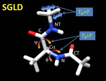
Alanine dipeptide is a basic building block of proteins. As shown in Fig.1, the conformation of this molecule is mainly characterized by two dihedral angles, ϕ: CT-N-Cα-C and ψ: N-Cα-C-NT. Even for such a small molecule, there are high frequency motions such as bond stretching, and low frequency motions such as the ϕ, φ dihedral angle changing. In LD simulations, all motions have the same temperature. In SGLD simulations, the low frequency motions are enhanced to help to accelerate conformational search.

Fig.1.

An alanine dipeptide and its motions in LD and SGLD simulations. Motions are marked by colored arrays with blue, yellow, and red to represent cold, normal, and hot temperatures. T_lf and T_hf represent low frequency temperature and high frequency temperature, respectively.

The CHARMM all-atom force field¹⁴ was used to describe the interactions. For simplicity we took a distance-dependent dielectric constant of 4r to represent solvent screening effects. Non-bonded interactions were calculated without a cutoff.

All simulations were performed with a time step of 2 fs and the SHAKE algorithm¹⁵ was employed to fix the bond lengths. Each simulation lasted 20 ns and conformations of every 2 ps were saved for post-analysis. All simulations were performed at 300 K except for high temperature LD simulations. A collision frequency of 10/ps was used for all the simulations. The SGLD and SGLD-GLE simulations were performed with a local average time of t_L=0.2 ps.

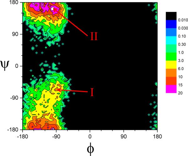
Fig.2 shows the ϕ-φ distributions obtained in a LD simulation at 300K. There are two major peaks as marked as I:(−90°,−70°) and II:(−90°, 160°). The frequency of transitions between the two peaks is used to measure the conformational sampling efficiency.

Fig.2.

the ϕ-φ distributions of an alanine dipeptide obtained from a 20 ns LD simulation at T=300 K, ξ=10/ps. Two popular regions, I around (−90°,−70°) and II around (−90°, 160°), are identified.

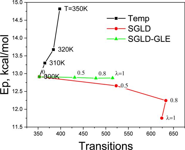
The transition between I and II has a small energy barrier. Many methods that increase the ability to overcome energy barriers often cause deviations in conformational distribution, reflected, e.g., in a change in average potential energy. Fig.3 shows the average potential energy vs the number of transitions achieved in high-temperature LD, SGLD, and SGLD-GLE simulations. As can be seen, elevated temperature shifts conformational sampling toward high energy conformations. In SGLD simulations, the guiding factor causes slow motions be enhanced and high frequency motion be suppressed. When applying SGLD method, there is an option to remove net guiding forces on the center of mass to avoid acceleration of the center of mass. Since this option is not available in SGLD-GLE, for the purpose of comparison the SGLD simulations reported here were performed without removing the net guiding force. As a result, the guiding effect shifts the sampling toward lower energy conformations, because more kinetic energy is distributed to the center of mass while less is distributed to internal motion, as seen in Fig. 3. Compared with high-temperature LD, SGLD increases the number transition much more effectively while causing much less deviations in the average potential energy. Fig.3 also shows the SGLD-GLE results. With λ increasing from 0 to 1, the number of transitions increases from 353 to 515, while the potential energy remains almost constant. While significant, the enhancement in conformational sampling is less than that of SGLD simulations with the same guiding factor. However, SGLD-GLE at λ=1 does much better than LD, and even much better than high-temperature LD.

Fig.3.

Average potential energies of the alanine dipeptide vs transitions between the the two ϕ–φ regions in high temperature LD, SGLD, and SGLD-GLE simulations. All the SGLD and SGLDGLE simulations were performed at T=300K with ξ=10/ps.

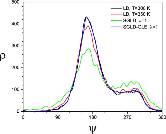
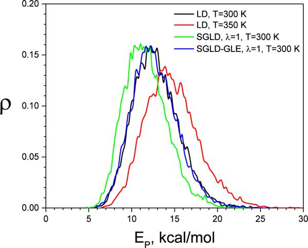
Fig.4 shows the φ angle distribution from these simulations. As can be seen, high-temperature LD and SGLD have flattened distributions, while the SGLD-GLE simulation produces almost exactly the same distributions as the LD simulation. Fig. 5 shows the potential energy distribution. Again, significant changes are observed in the high-temperature LD and SGLD results, whereas the SGLD-GLE result almost overlaps with the LD result. This confirms that SGLDGLE samples exactly the canonical distribution.

Fig.4.

The φ angle distributions of the alanine dipeptide in the LD, SGLD, and SGLD-GLE simulations. All simulations were performed at T=300K, ξ=10/ps except the high temperature LD performed at T=350 K.

Fig.5.

The potential energy distribution of the alanine dipeptide in LD at T=300K and T=350K, SGLD, and SGLD-GLE simulations at T=300K, ξ=10/ps, and λ=1.

Liquid argon

Next we use an argon fluid to further examine the application of SGLD-GLE in the NPT ensemble. Argon atoms are described by the Lennard-Jones 6-12 potentials with ε=119.8K and σ=3.405Å. 500 argon atoms were placed in a cubic periodic box (28.53×28.53×28.53 ų). A collision frequency of 10 ps⁻¹ and a time step of 1 fs were used for all simulations. All the SGLD and SGLD-GLE simulations were performed at 100 K. The target pressure was 1 atm. Each simulation lasted 10 ns. Coordinates and velocities of every 0.05 ps were stored for post analysis.

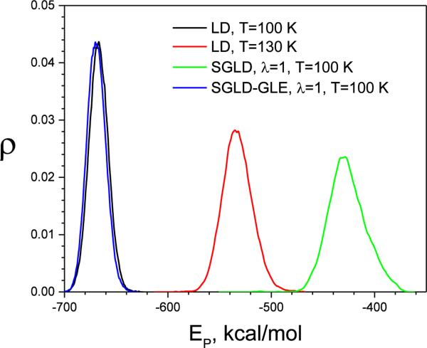
Conformational distributions are again compared through the potential energy distributions from LD, SGLD, and SGLD-GLE simulations. As can be seen from Fig.6, high-temperature LD significantly shifts the sampling to high energy conformations, while SGLD-GLE has an energy distribution that is almost identical to that of the LD simulation. For SGLD, at such a high friction constant and guiding factor, conformational distribution also shits toward high energy area.

Fig.6.

The potential energy distributions of the liquid argon from LD, SGLD, and SGLD-GLE simulations. All simulations were performed at T=100 K, ξ=10/ps, except that the high temperature LD simulation that was performed at T=150 K. The guiding factor was λ=1 for both the SGLD and SGLD-GLE simulations.

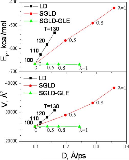
An accelerated conformational sampling corresponds to an increase in diffusion constant. We can compare the average energy and average volume as functions of the diffusion constant to examine the efficiency to accelerate conformational sampling. Fig. 7 plots the average energies and volumes against the diffusion constants achieved in these simulations. Clearly, temperature elevation caused fastest energy and volume increases. SGLD caused smaller changes in average energies and volumes with the same increase in diffusion constants. SGLD-GLE resulted in almost identical average energies and volumes to the LD simulation, while achieving significantly large diffusion constants.

Fig.7.

The average potential energies and volumes of argon liquid are plot against the diffusion constants in high temperature LD, SGLD, and SGLD-GLE simulations. All simulations were performed at ξ=10/ps, T=100 K and P=1 atm except labeled otherwise. The high-temperature LD simulations are labeled with temperatures. The SGLD and SGLD-GLE simulations were labelled with the guiding factors.

The dynamic property of simulated systems can be understood from the spectrum of velocity auto-correlation function. We use the following equation to calculate the spectrum.

$$\rho \left(\omega \right)={\int }_{-\infty }^{\infty }C\left(t\right)\exp (-i\omega t)dt$$ (20)

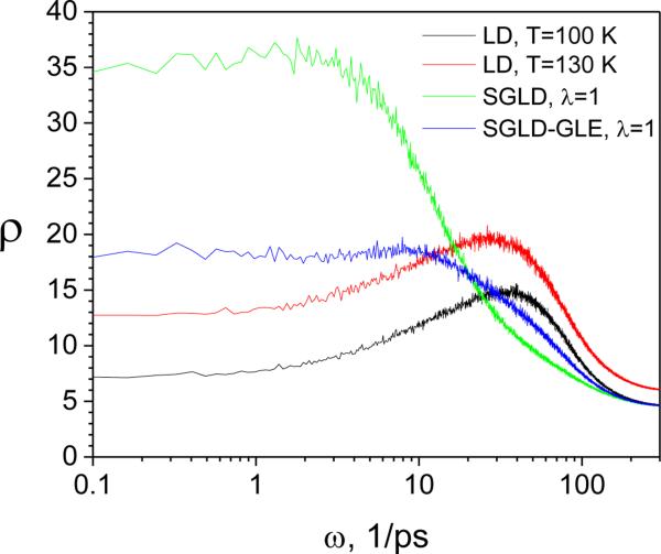
where C(t) is the velocity auto-correlation. Fig.8 shows the spectra from LD simulations at different temperatures, as well as that from SGLD and SGLD-GLE simulations at T= 100K. As the temperature increases from 100K to 130K, the spectrum shifts upward at all frequencies. This result indicates that increasing temperature will enhance the motion of all frequencies. Comparing the spectra from LD, SGLD, and SGLD-GLE at the same temperature (T=100 K), we can see that SGLD and SGLD-GLE enhance the slow motions (low frequencies) and reduce fast motions (high frequencies). A longer averaging time (a larger t_L) results in slower motions being further enhanced^1-3. The guiding factor determines the increase in the diffusion constant, while the averaging time determines the portion of motion to be enhanced. From the spectrum at the lowest frequency, it is clear that SGLD increases the diffusion constant, which is what leads to the enhanced efficiency in conformational search.

Fig.8.

The spectrum of the argon liquid from LD, SGLD, and SGLD-GLE simulations. All simulations were performed at T=100 K, P=1 atm, and ξ=10/ps, except that the high temperature LD was performed at T=150 K. The guiding factor was λ=1 for the SGLD and SGLD-GLE simulations.

Concluding Remarks

SGLD-GLE is a modification of SGLD in which a generalized Langevin equation is used to restore the detailed-balance property of the dynamics. This permits to sample the NVT and NPT ensembles exactly, without the reweighting needed in SGLD. The usefulness of the method was illustrated via two examples, alanine dipeptide and liquid argon, which showed that SGLD-GLE (i) is accurate in conformational sampling and (ii) has enhanced sampling efficiency in both the NVT and NPT ensembles.

We should stress that in these tests, we compared the performance of SGLD-GLE to that of standard LD. Since the guiding force defined in eq.(15) is proportional to the friction constant, γ, the improvement of efficiency of SGLD-GLE over LD is more pronounced when γ is large. This is consistent with the fact that SGLD-GLE enhances conformational search through reduction of the damping effect due to the friction forces, and, therefore, becomes comparable to LD in the limit as γ → 0. This limit, however, will typically not be the one that optimizes the speed of sampling, and therefore we expect that SGLD-GLE will be superior to LD when it matters, i.e. when the sampling is performed at finite γ.

We should also stress that, while SGLD-GLE performs exact sampling and does not need re-weighting like standard SGLD, this comes at a price: indeed, the modification of the force used to restore detailed-balance typically reduces the overall acceleration of the method compared to that of SGLD. Thus SGLD may be preferred if conformational exploration is the main objective, while SGLD-GLE is the appealing alternative to LD if conformational sampling is the goal. In these situations, it will provide an appealing alternative to LD.

Compared with other sampling enhancement methods, SGLD-GLE has several unique characters. First, SGLD-GLE is size extensive. The guiding force is calculated from momentum and random forces, independent of system size. Reweighting is no longer needed which allows the method to be cast in a manner that is size extensive, making it a possible method of choice for million atom systems that may benefit from enhanced sampling. Second, the method can be applied to a part of a simulation system. In other words, the guiding factor can be defined for individual atoms, just like the friction constant can be atom specific. Third, the motion mode to be enhanced can be controlled by the local averaging time. Because of these features, we expect that SGLD-GLE, like SGLD, will be useful in a wide variety of contexts, such as phase transition, ligand docking, and protein folding.

Appendix

To prove that eq.(18) is the solution to the FPE in eq.(17), let us denote

$$z=\left(\begin{array}{c}\hfill \left\{{\mathbf{r}}_i\right\}\hfill \\ \hfill \left\{{\mathbf{p}}_i\right\}\hfill \\ \hfill \left\{{\mathbf{g}}_i\right\}\hfill \end{array}\right)$$ (A1)

Let us also introduce:

$$\begin{array}{cc}\hfill & w\left(z\right)=E_{\mathrm{p}}+\sum _i(\frac{{\mid {\mathbf{p}}_i\mid }^2}{2m_i}+\frac{t_{\mathrm{L}}{\mid {\mathbf{g}}_i\mid }^2}{2m_i\gamma {\mu }^2})\hfill \\ \hfill & \text{and}\sigma =\sqrt{kT{m}_i{\mathbf{g}}_i}\left(\begin{array}{c}\hfill 0\hfill \\ \hfill 1\hfill \\ \hfill -\mu ∕t_{\mathrm{L}}\hfill \end{array}\right),\text{so that}:\hfill \end{array}$$ (A2)

$$\sigma {\sigma }^{\mathrm{T}}=kT{m}_i{\mathbf{g}}_i\left(\begin{array}{c}\hfill 0\hfill \\ \hfill 1\hfill \\ \hfill -\mu ∕t_{\mathrm{L}}\hfill \end{array}\right)\left(\begin{array}{ccc}\hfill 0\hfill & \hfill 1\hfill & \hfill -\mu ∕t_{\mathrm{L}}\hfill \end{array}\right)=kT\omega$$ (A3)

where

$$\omega =m_i{\mathbf{g}}_i\left(\begin{array}{ccc}\hfill 0\hfill & \hfill 0\hfill & \hfill 0\hfill \\ \hfill 0\hfill & \hfill 1\hfill & \hfill -\mu ∕t_{\mathrm{L}}\hfill \\ \hfill 0\hfill & \hfill -\mu ∕t_{\mathrm{L}}\hfill & \hfill {\mu }^2∕t_{\mathrm{L}}^2\hfill \end{array}\right)$$ (A4)

Finally, let us define an antisymmetric matrix:

$$\kappa =\left(\begin{array}{ccc}\hfill 0\hfill & \hfill 1\hfill & \hfill 0\hfill \\ \hfill -1\hfill & \hfill 0\hfill & \hfill m_i{\mathbf{g}}_i\mu (\mu -1)∕t_{\mathrm{L}}\hfill \\ \hfill 0\hfill & \hfill -m_i{\mathbf{g}}_i\mu (\mu -1)∕t_{\mathrm{L}}\hfill & \hfill 0\hfill \end{array}\right)$$ (A5)

κ is antisymmetric: κ = –κ^T.

In terms of these quantities, the GLE, eq.(7), used in SGLD-GLE can be written as:

$$\stackrel{.}{z}=-\omega {\nabla }_{z}w+\kappa {\nabla }_{z}w+\sqrt{kT}\sigma \eta \left(t\right)$$ (A6)

Here, η(t) is a vectorial white-noise. The FPE associated with this equation is eq.(17) which can be written as:

$${\nabla }_z\left[(\omega -\kappa ){\nabla }_{z}w\rho +kT\omega {\nabla }_z\rho \right]=0$$ (A7)

To check that eq.(18), that is ρ = e^–w/kT, solves this equation, notice that:

$$1).\omega {\nabla }_{z}w\rho +kT\omega {\nabla }_z\rho =\omega {\nabla }_z\omega \rho +kT\omega \left(-\frac{1}{kT}{\nabla }_{z}w\rho \right)=0$$ (A8)

$$2).{\nabla }_2\kappa {\nabla }_{2}w\rho =\kappa {\nabla }_z{\nabla }_{z}w\rho -\frac{\kappa }{kT}{\nabla }_{z}w{\nabla }_{z}w\rho =0,$$ (A9)

because κ is antisymmetric.

References

- 1.Wu X, Brooks BR. Chemical Physics Letters. 2003;381:512–518. [Google Scholar]
- 2.Wu X, Brooks BR. J Chem Phys. 2011;134:134108. doi: 10.1063/1.3574397. [DOI] [PMC free article] [PubMed] [Google Scholar]
- 3.Wu X, Damjanovic A, Brooks BR. In: Advances in Chemical Physics. Rice SA, Dinner AR, editors. Vol. 150. John Wiley & Sons, Inc.; Hoboken: 2012. pp. 255–326. [DOI] [PMC free article] [PubMed] [Google Scholar]
- 4.Damjanovic A, Wu X, Garcia-Moreno E B, Brooks BR. Biophysical Journal. 2008;95:4091–4101. doi: 10.1529/biophysj.108.130906. [DOI] [PMC free article] [PubMed] [Google Scholar]
- 5.Damjanovic A, Miller BT, Wenaus TJ, Maksimovic P, Bertrand Garcia-Moreno E, Brooks BR. Journal of Chemical Information and Modeling. 2008;48:2021–2029. doi: 10.1021/ci800263c. [DOI] [PubMed] [Google Scholar]
- 6.Damjanović A, GarcÃa-Moreno E B, Brooks BR. Proteins: Structure, Function and Bioformatics. 2009;76:1007–1019. doi: 10.1002/prot.22439. [DOI] [PMC free article] [PubMed] [Google Scholar]
- 7.Pendse PY, Brooks BR, Klauda JB. Journal of Molecular Biology. 2010;404:506–521. doi: 10.1016/j.jmb.2010.09.045. [DOI] [PMC free article] [PubMed] [Google Scholar]
- 8.Lee CI, Chang NY. Biophysical Chemistry. 2010;151:86–90. doi: 10.1016/j.bpc.2010.05.002. [DOI] [PubMed] [Google Scholar]
- 9.Wu X, Brooks BR. J Chem Phys. 2011;135:204101. doi: 10.1063/1.3662489. [DOI] [PMC free article] [PubMed] [Google Scholar]
- 10.Zwanzig R. Physical Review. 1961;124:983–992. [Google Scholar]
- 11.Ceriotti M, Bussi G, Parrinello M. Phys Rev Lett. 2009;102:020601. doi: 10.1103/PhysRevLett.102.020601. [DOI] [PubMed] [Google Scholar]
- 12.Ceriotti M, Bussi G, Parrinello M. Journal of Chemical Theory and Computation. 2010;6:1170–1180. [Google Scholar]
- 13.Marchesoni F, Grigolini P. The Journal of Chemical Physics. 1983;78:6287–6298. [Google Scholar]
- 14.Brooks BR, Brooks Iii CL, Mackerell Jr AD, Nilsson L, Petrella RJ, Roux B, Won Y, Archontis G, Bartels C, Boresch S, Caflisch A, Caves L, Cui Q, Dinner AR, Feig M, Fischer S, Gao J, Hodoscek M, Im W, Kuczera K, Lazaridis T, Ma J, Ovchinnikov V, Paci E, Pastor RW, Post CB, Pu JZ, Schaefer M, Tidor B, Venable RM, Woodcock HL, Wu X, Yang W, York DM, Karplus M. Journal of Computational Chemistry. 2009;30:1545–1614. doi: 10.1002/jcc.21287. [DOI] [PMC free article] [PubMed] [Google Scholar]
- 15.Ryckaert JP, Ciccotti G, Berendsen HJC. J.Comput.Phys. 1977;23:327–341. [Google Scholar]