A female pelvic bone shape model for air/ bone separation in support of synthetic CT generation for radiation therapy

Abstract

Separating bone from air in MR data is one of the major challenges in using MR images to derive synthetic CT. The problem is further complicated when the anatomic regions filled with air are altered across scans due to air mobility, for instance, in pelvic regions, thereby the air regions estimated using an ultrashort echo time (UTE) sequence are invalid in other image series acquired for multispectral classification. This study aims to develop and investigate a female pelvic bone shape model to identify low intensity regions in MRI where air is unlikely to be present in support of synthetic CT generation without UTE imaging. CT scans of 30 patients were collected for the study, 17 of them also have corresponding MR scans. The shape model was built from the CT dataset, where the reference image was aligned to each of the training images using B-spline deformable registration. Principal component analysis was performed on B-spline coefficients for a compact model where shape variance was described by linear combination of principal modes. The model was applied to identify pelvic bone in MR images by deforming the corresponding MR data of the reference image to target MR images, where the search space of the deformation process was constrained within the subspace spanned by principal modes. The local minima in the search space were removed effectively by the shape model, thus supporting an efficient binary search for the optimal solution. We evaluated the model by its efficacy in identifying bone voxels and excluding air regions. The model was tested across the 17 patients that have corresponding MR scans using a leave-one-out cross validation. A simple model using the first leading principal mode only was found to achieve reasonable accuracy, where an averaged 87% of bone voxels were correctly identified. Finally dilation of the optimally fit bone mask by 5 mm was found to cover 96% of bone voxels while minimally impacting the overlap with air (below 0.4%).

1. Introduction

Several different methods have been recently proposed to generate attenuation maps and synthetic CT of patients using magnetic resonance imaging (MRI) data (Chen et al 2007, Johansson et al 2011, Greer et al 2011, Lambert et al 2011, Dowling et al 2012, Kim et al 2012, Kapanen et al 2013, Hsu et al 2013, Korhonen et al 2014, Uh et al 2014, Kim et al 2015), with the aim of removing the need for computed tomography (CT) scans to support attenuation correction of positron emission tomography (PET) in a PET-MRI system, radiation dose calculation and some aspects of image guidance in radiation therapy. One class of these methods generates electron density maps based on the alignment between an atlas derived from reference CT images and the target MR images (Greer et al 2011, Dowling et al 2012, Uh et al 2014). However, such methods are somewhat limited in their ability to adapt to patient anatomical variations, a problem that is exacerbated in the female pelvis as compared to the male pelvis.

In more individualized approaches, a relation between the attenuation properties and image intensities of one or more MRI scans is developed and applied to generate ‘synthetic’ CT images (Johansson et al 2011, Kim et al 2012, Hsu et al 2013). One major challenge of individualized methods is the difficulty in separating bone from air in MR data due to its short T2/T2*. Ultrashort echo time scanning techniques, such as ultrashort echo time (UTE) and pointwise encoding time reduction with radial acquisition (PETRA) are able to yield signals from tissues with short T2. While intensity thresholding of UTE image data to mask air in support of synthetic CT generation has been evaluated and validated for attenuation mapping in the head (Hsu et al 2015), this process is challenging in the pelvis due to the mobility of air over short time periods. Intra-session changes may lead to air regions estimated from UTE not spatially matching the locations of air in other MR volumes from the same scanning session. This potential spatial mismatch could lead to misclassification of air as bone in the pelvis. Several methods (Chen et al 2007, Kapanen et al 2013, Korhonen et al 2014, Kim et al 2015) manually contoured the bony part in pelvis before synthetic CT generation, which can be time-consuming and non-repeatable.

One approach to address this issue is to add bone shape information to assist the air/bone separation process. As air is rarely in close contact with bone in the pelvis, defining the space in which bone exists would allow for identifying air in remaining low MR intensity regions outside of bone for exclusion from tissue classification (e.g. Hsu et al 2013), and thus also remove the need for ultrashort TE imaging. Achieving this goal requires a model that describes possible shape variance of the pelvic bone. Various methods have been proposed for shape model construction, including (1) active shape models where shape variability is represented by the variance of coordinates of landmarks placed on the object (Cootes et al 1995, Schmid et al 2008); (2) active contour models where shape variability is represented by the variance of object contours (Leventon et al 2000, Tsai et al 2003); (3) statistical deformation models where shape variability is represented by a series of deformation fields that deform a reference image to match a group of training images (Chintalapani et al 2007, Thompson et al 2008, Gao et al 2013). As compared to active shape models and active contour models, statistical deformation models do not require explicit contouring of objects, and are thus less expensive in terms of effort for model construction. In this study, a pelvic bone shape model is developed and investigated based upon deformable alignment of pelvic CT image volumes across a female population to assist bone identification in MRI as the first step in the synthetic CT generation. As actual attenuation values will be determined in a subsequent probabilistic tissue classification step that permits voxels to have combinations of tissues, the goal here is to find a bulk space where air is unlikely to exist instead of contouring bone tissues accurately. This reduced demand for specificity in bone location labeling allows a trade-off between model accuracy versus model complexity. As compared to deformable registration based methods (Greer et al 2011), the shape model has fewer parameters to be optimized and the search space appears to be free of local minima, thus is more computational efficient and robust.

2. Method and materials

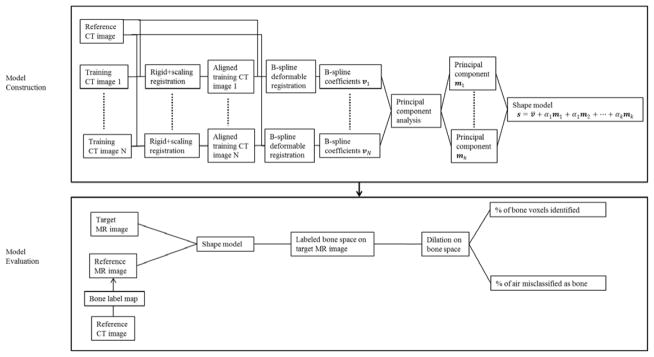
We built the model from CT images where bone structure can be easily defined, and applied it to MR images for model evaluation. To exclude individual differences that are not due to shape variance, all images were first (rigidly plus scale) aligned into the same coordinate system. The reference CT was deformably aligned to the resulting images, and Principal Component Analysis (PCA) of the population of deformations was used to assemble the shape model. The shape model was then used to guide the deformation of the reference MR image with labeled bone regions to match the target MR image. Dilation was further introduced to improve the coverage of bone voxels. Figure 1 shows a flow chart of the model construction and application/evaluation processes.

Figure 1.

Flow chart showing the model construction and evaluation processes.

2.1. Image data for shape model construction

Under institution review board approval, CT image volumes acquired from 30 female patients who underwent simulation for external beam radiotherapy were investigated. Of these patients, 17 also had corresponding MR scans. CT scans were acquired with slice thickness of 3 mm and in-plane pixel size of 1 × 1 mm². MR scans included T1-weighted images were generated using a 3D gradient echo sequence (VIBE Dixon, initially designed for breath-hold liver imaging) with TE (in/out-of-phase) equals 2.46/1.23 ms, TR equals 4.1 ms, flip angle 9°, and voxel size of 1.5 × 1.5 × 1.5 mm³. Fat and water images were computed from the in-phase (T1-weighted) and out-of-phase VIBE images. All MR and CT images were acquired using a 3T MR scanner (Skyra, Siemens Medical Systems, Erlangen, Germany) and CT simulator (Philips Healthcare, Cleveland, OH), respectively. The CT scans were done with 120 kVp and 450 mAs. All scans were acquired with patients lightly immobilized in vacuum-formed bean bags, and with no other controls on physiological movement. Intensity inhomogeneity correction was applied to MR images using a N4 algorithm (Tustison et al 2014), implemented in a publicly available image analysis software environment (SLICER, surgical processing laboratory, Brigham and Women’s Hospital, Boston, MA). All MR images were aligned to their corresponding CT images through rigid registration implemented in SLICER. This task was trivial as the MR and CT scans come from the same patient. All image volumes were reformatted in axial orientation with voxel sizes interpolated to 1 × 1 × 1 mm³. Example images used from one subject are shown in figure 2. Variations in subject body composition as well as internal motion during scans were present in the study population. Figure 3 shows one sample image from the dataset that shows motion artifacts as well as one sample image that has relatively high quality.

Figure 2.

Example MR and CT images from one study subject. (a) T1-weighted (in-phase), (b) fat, (c) water and (d) CT image.

Figure 3.

Example T1-weighted MR images used for this study with different image qualities. Left: image that shows motion artifacts (lines indicated by red arrows). Right: image of relatively high quality.

2.2. Model construction

2.2.1. Alignment of training images

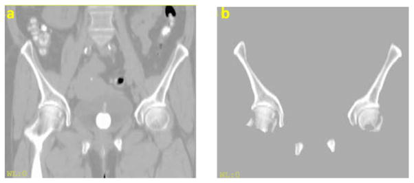
Since we were interested in bone identification only, irrelevant structures were first excluded to reduce alignment complexity. Bony surfaces were identified on CT images using an intensity threshold of 150 Hounsfield units (HU). These surfaces were dilated by 3 mm to include contrast with adjacent surrounding soft tissues. Using an in-house Functional Imaging Analysis Tool (FIAT), morphological operations (3 mm dilation, filling holes and 3 mm erosion) were subsequently applied to clean up holes and gaps. Non-pelvic bones, such as vertebrae and femurs, were manually removed. Example CT images before and after preprocessing are shown in figure 4.

Figure 4.

CT image (a) before and (b) after preprocessing.

After the above preprocessing steps, one CT image volume was selected randomly from the dataset as the reference. To exclude individual differences that were not due to shape variance, the remaining training images in the dataset were first aligned to the reference image using rigid registration plus global scaling. Then the reference image was deformed to match each of the training images, using a multilevel B-spline deformable registration with subsampling rates of [10 10 5], [4 4 2] and [2 2 1] voxels and B-spline grid sizes of 50, 30 and 15 mm respectively. The regularization parameter for smoothness was 0.005 and the maximal number of iterations was 50 for each level. The mean square error between the target and reference image was chosen as the similarity metric for both rigid and B-spline deformable registration processes. Four anatomic landmarks were identified at the top and the bottom and the left and the right of the pelvis, as shown in figure 5, to initialize the rigid plus scaling alignment. All alignments were performed using SLICER. Figure 6 shows the reference image as well as an example deformation field that warps the reference image to match a training image.

Figure 5.

Landmarks placed on CT image volumes to assist alignment.

Figure 6.

(a) Reference image. (b) Target image with deformation vectors. (c) Deformed reference image.

2.2.2. Principal component analysis of B-spline coefficients

To extract representative modes of shape variance, PCA is usually performed on a matrix composed of deformation fields obtained from the non-rigid alignment process. The deformation fields in our method were calculated from B-spline coefficients at control points through simple interpolation, and thus the high dimensional deformation fields were mapped from the low dimensional B-spline coefficients through a linear transformation matrix. Therefore the information encoded in deformation vectors and B-spline coefficients is equivalent. PCA was performed on the B-spline coefficients instead of the deformation vectors to yield more compact descriptions of shape variance and save computational effort by reducing the matrix size.

The B-spline coefficients of the ith deformation field were organized into a vector v_i and PCA was performed on the matrix

$$\mathbf{V}=[{\mathit{v}}_1,{\mathit{v}}_2,\cdots ,{\mathit{v}}_{\mathit{N}}]$$ (1)

PCA of V yields N orthogonal principal modes m₁, m₂, ···, m_N. This gives the shape model where the possible shape variance s of pelvic bone is described by a linear combination of the leading k principal modes plus the mean B-spline coefficients v̄

$$\mathbf{s}=\overline{\mathit{v}}+{\alpha }_1{\mathit{m}}_1+{\alpha }_1{\mathit{m}}_2+\cdots +{\alpha }_k{\mathit{m}}_k$$ (2)

2.3. Application of model to identify pelvic bone in MR images

2.3.1. Deformable alignment guided by shape model

To identify pelvic bone on MR images, we deformed the corresponding MR data of a reference image A to match a target image M. The bone regions on the reference MR image were identified and labeled according to the corresponding CT image. The deformation process was guided by the shape model developed in 2.2 by constraining the search space to be within the space spanned by principal modes. The problem can be formulated as

$$\begin{array}{l}\widehat{\mathit{\alpha }}=arg\underset{\mathit{\alpha }}{min}D(\mathbf{T}(\mathbf{A}),\mathbf{M})\\ \text{such}\text{that}\mathbf{T}=\mathbf{B}(\mathit{v}),\mathit{v}=\overline{\mathit{v}}+{\alpha }_1{\mathit{m}}_1+{\alpha }_1{\mathit{m}}_2+\cdots +{\alpha }_k{\mathit{m}}_k\end{array}$$ (3)

where D is the similarity metric between the target and reference images and T is the deformation field that is calculated from B-spline coefficients v at control points using the cubic B-spline interpolator B. By using the subspace model (2), we only need to optimize over the k model coefficients (α₁, ···, α_k). As compared to deformable registration, our model has far fewer parameters involved in the optimization process.

In our approach, we chose the mean square intensity error between the reference and the target water images as the similarity metric D. The images were first normalized based on the mean intensity of the T1-weighted images from the same acquisition that yielded the water images. Since we were interested in pelvic bone only, the value of the similarity metric was evaluated only in the regions where the deformed reference image indicated the existence of bone (i.e. fell within the labeled bone space on the reference image). The optimization problem was thus

$$\begin{array}{l}\widehat{\mathit{\alpha }}=arg\underset{\mathit{\alpha }}{min}\sum _{\mathbf{T}(\mathbf{A}(x))\in \text{bone}}{(\mathbf{T}(\mathbf{A}(\mathit{x}))-\mathbf{M}(\mathit{x}))}^2\\ \text{such}\text{that}\mathbf{T}=\mathbf{B}(\mathit{v}),\mathit{v}=\overline{\mathit{v}}+{\alpha }_1{\mathit{v}}_1+{\alpha }_1{\mathit{v}}_2+\cdots +{\alpha }_k{\mathit{v}}_k\end{array}$$ (4)

With the binary operator introduced by the masked bone space, the optimization problem in equation (4) is not differentiable. Given the small number of parameters, we may simply traverse a grid of parameter values to find the optimal solution. Furthermore, if we assume the uniqueness of minimum of the search space, a binary search scheme may be used to find the optimal coefficients efficiently.

2.4. Evaluation and validation

We evaluated the shape model by calculating the percentage of correctly identified bone voxels as well as the percentage of air being misclassified as bone, where air voxels were defined on corresponding CT images at a threshold of −400 HU. For each of the 17 patients that had both MR and CT scans, we constructed the shape model from the remaining 29 CT scans and applied the model to identify pelvic bone on the MR image of the patient whose CT was not used in the model development. To evaluate the complexity of the search space, we calculated the objective function values by brute force sampling of coefficients of the first three principal modes. To validate the choice of similarity metric, the model was fitted to CT data by directly maximizing the percentage of identified bone voxels, as the bone label map was already defined on CT images, and compared to the result when applying the model to MR images. Finally, the effect of dilation on the identified space was studied by evaluating both the percentage of correctly identified bone voxels and the percentage of air voxels mislabeled as bone.

3. Results

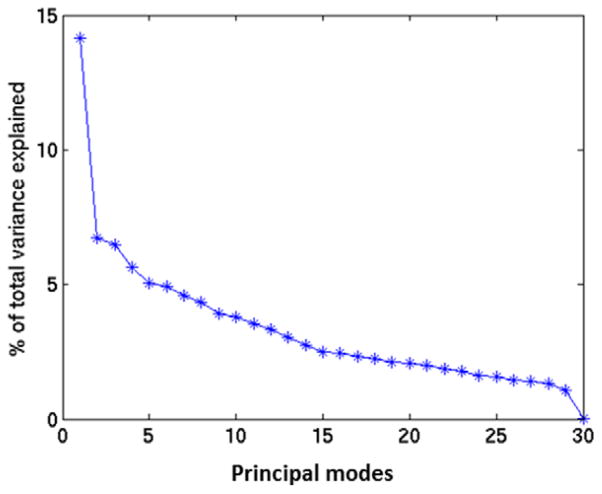
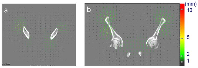
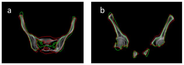
The B-spline coefficients with in pelvic bone area ranged from −41.27 to 49.71, with a mean of −0.24, standard deviation of 8.33 and a mean absolute of 6.35. The percentage of total variance of deformations (B-spline coefficients) across patients explained by each mode is shown in figure 7. The first leading mode accounts for 14% of the total variance. Figure 8 shows the deformation field corresponding to the first principal mode and figure 9 shows the reference image deformed by the first principal mode by varying the coefficients between 5 (red contour) and −15 (green contour) of the standard deviation of the population.

Figure 7.

Percentage of variance explained by each mode.

Figure 8.

Deformation fields corresponding to the first principal mode with the reference image in the (a) axial plane and (b) coronal plane.

Figure 9.

Contours of two deformation samples (red and green) using the first principal mode with the respective coefficients of 5 and −15 of the standard deviation of the population, with the reference CT images (grey) in the axial (left) and coronal plane (right).

We explored the properties of the search space by plotting the objective function values under various model coefficients, as shown in figure 10. The objective function was observed to be free of local minima, thus justifying adoption of a binary search scheme to find the optimal model coefficients more efficiently than brute force or more complex searching schemes. Details of the binary search algorithm can be found in the appendix.

Figure 10.

Plot of the objective function values with (a) the coefficients of the 2nd versus 3rd principal mode at the optimal value for the coefficient of the 1st principal mode, (b) the coefficients of the 1st versus 3rd principal mode at the optimal value for the coefficient of the 2nd principal mode, and (c) the coefficients of the 1st versus 2nd principal mode at the optimal value for the coefficient of the 3rd principal mode.

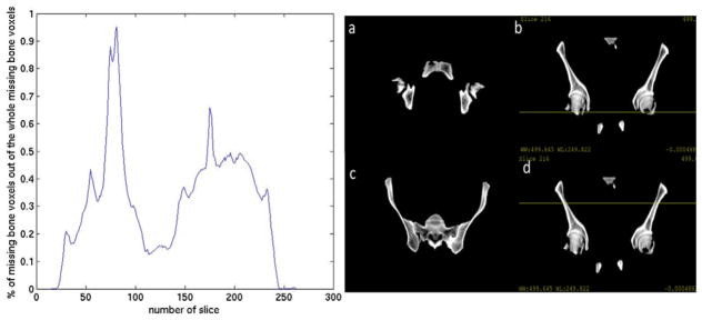
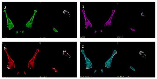
Using the first leading principal mode only, the leave-one-out cross validation process achieved an averaged bone identification rate of 87% across 17 patients. The lowest coverage was 79% and the highest coverage was 94%. The standard deviation across the 17 patients was 6%. The averaged total volumes of unidentified bone were 118.33 cm³ and the standard deviation of unidentified bone volumes was 70.77 cm³. The averaged percentage of air voxels misclassified as bone was 0.02% and the standard deviation across patients was 0.08%. The averaged total volumes of misclassified air were 0.23 cm³ and the standard deviation of misclassified air volumes was 0.70 cm³. For most patients, the largest portions of missing bone voxels were located at the bottom (femoral head) and top of the segmented pelvis. Figure 11 shows the averaged portion of missing bone voxels of the total amount of missing bone voxels in each slice (axial plane). The peaks appear around slice 81 and slice 175. Figure 11 also shows the two axial slices of the reference image as well as a coronal view with yellow lines indicating the position corresponding to the specific axial slice. This trend could be due to the bias introduced by the selected reference image and (in the case of the femoral heads) somewhat arbitrary means of cutting off the more distal bone from the segmentation. The spinal elements attached to the pelvis further contributed to misclassified bone voxels (20% of the total misclassified bone voxels) as the model was initially developed to describe pelvic bone shape only. Figure 12 shows examples of the identified bone voxels overlapped with the ground truth CT images for 4 patients where the model achieves the best performance, average performance and worst performance.

Figure 11.

Analysis of the location of missing bone voxels. Left: percentage of missing bone voxels in each axial slice, two peaks appear at slice 81 and slice 175. Right: (a) axial slice 81 of the reference image. (b) Coronal plane with yellow line corresponding to axial slice 81. (c) Axial slice 175 of the reference image. (d) Coronal plane with yellow line corresponding to axial slice 175.

Figure 12.

Example pelvic CT images with color wash indicating bone voxels identified by the deformed reference image for 4 patients that have different model performances: (a) patient that has bone coverage of 93%. (b) Patient that has bone coverage of 94%. (c) Patient that has bone coverage of 85%. (d) Patient that has bone coverage of 79%.

The optimal model coefficient found for each of the 17 patients ranged from 87 to −350, with a mean of −28 and a standard deviation σ = 211. The averaged maximal decreases (when compared to individual optimizations) in bone coverage when varying the model parameter by ±1.5σ and ±1σ around the mean were 9.7% and 6.3% across these 17 patients, respectively. These added errors are large compared to the coverage with the first mode, and suggest that the variation across individuals warrants the use of some deformation to achieve a reasonable tradeoff of sensitivity and specificity in bone/air separation. On the other hand, varying the model parameter by ±0.5σ around the optimal model parameter found for each patient decreased the model performance by 1.6% only, indicating the model is robust to small deviations from the true optimum. It is possible in the future to use this added knowledge to permit an even faster search for the optimal combination of deformation model and marginal expansion.

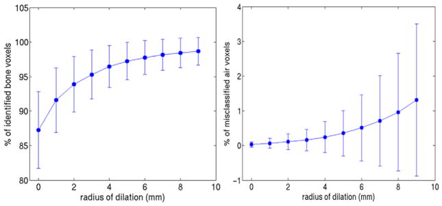
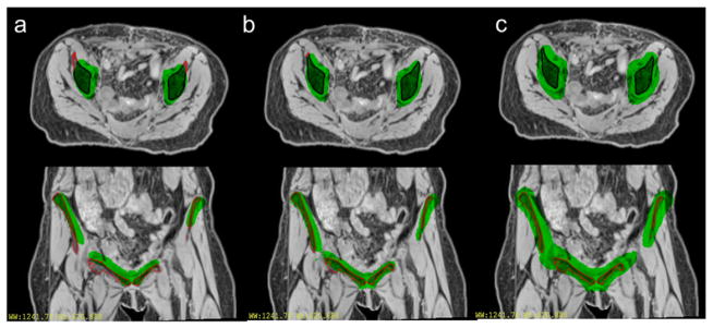
Fitting the model to CT data using the first leading mode, the leave-one-out cross validation achieved an average bone identification rate of 88%, which is similar to the result obtained from MR, thus validating our choice of the mean square error as the optimization criterion. Figure 13 shows the averaged percentage of correctly identified bone voxels by fitting the model to MRI data as well as the percentage of mislabeled air voxels versus radius of dilation of the identified bone space, with error bars specifying the standard deviation across the population. Dilating the space by 5 mm improved the overlap with true bone to 96%, while the percentage of air voxels mislabeled as bone remained below 0.4%. Figure 14 shows an example of the bone label of the reference image overlapped with one target image, before and after the model-guided deformation. The coverage of bone voxels in the target image was improved after the deformation and dilation further improved the bone coverage.

Figure 13.

Left: fraction of correctly identified bone voxels under various radius of dilation. Right: fraction of air voxels mislabeled as bone under various radius of dilation. The length of the error bar corresponds to the standard deviation across the population.

Figure 14.

Labeled regions (green) of the reference image overlapped with the target image (with red contours for bone region) (a) before deformation (b) after deformation and (c) applying a 5 mm dilation of the labeled region after deformation.

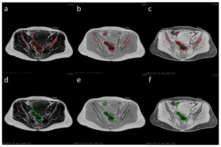
With the bone spaces identified by the shape model, the remaining dark spaces in MR images can be labeled as air and excluded from the following tissue classification process. The air spaces were identified by thresholding the MR images in non-bone spaces at intensity cutoffs of 300, 150 and 300 for the T1-weighted, water and fat images respectively. All images were normalized by the mean intensity of the T1-weighted images before thresholding. Examples of the thresholded MR images with and without the bone mask are shown in figure 15. Without the bone identification step, intensities of bone voxels and air voxels both fall below the threshold, resulting in mixture of air and bone. After the bone identification step, bone area was first masked out before thresholding and air regions were identified without mislabeling bone as air.

Figure 15.

(a)–(c) Thresholded fat, T1-weighted and water image without bone mask. Threholded regions were contoured by red lines. (d)–(f) Thresholded fat, T1-weighted and water image after bone identification. Thresholded regions were contoured by green lines.

Including the 2nd and 3rd principal modes into the model resulted in an averaged improvement in coverage of bone of less than 2% prior to dilation. After the 5 mm dilation was applied, the difference between the model with 3 modes and the model with 1 mode was only 0.06%. On the other hand, the model with 3 modes resulted in an air misclassification rate slightly higher than the model with 1 mode. The difference was 0.2% without dilation and 0.3% after the 5 mm dilation. This result suggests that using the 1st leading mode may achieve a sufficiently accurate model for separation of bone and air while maintaining simplicity and computational efficiency.

4. Discussion

In this study, we investigated a female bone shape model to facilitate bone identification as the first step in the workflow of synthetic CT generation from pelvic MR data. By identifying a space that contains the pelvic bones plus a small expansion, a simple intensity threshold can be applied to the remainder of voxels within the pelvis to exclude air voxels from the tissue classification process, without mislabeling bone as air. This permits classification of bone without the use of ultrashort TE imaging in the pelvis.

While previous investigations of pelvic shape model (Chintalapani et al 2007, Thompson et al 2008, Gao et al 2013) aimed at contouring bone structure accurately and evaluated the resulting models by surface distance, we focused on a simpler problem of identifying a region that contains bone and excludes air. Therefore we evaluated the model in terms of the coverage of bone and the overlap with air. Under this evaluation criterion, a single principal mode was observed to achieve sufficient accuracy, which reduced the model complexity as compared to most existing methods where more than 10 modes were typically involved. In comparison to results reported in existing work, our method gains computational efficiency where the one segmentation takes 69 s on average on a shared 2.8 GHz CPU with 40 cores (i.e. we do not specifically allocate all cores as other jobs run with equal priority), as compared to 2.5 h on an 8-core machine with a 3.2 GHz CPU as reported (Gao et al 2013). Spatial dilation was further introduced to improve the coverage of bone, while the overlap with air remained reasonably small even with a 5 mm dilation that covered 96% of pelvic bone voxels. By performing PCA on B-spline coefficients instead of deformation vectors, we were able to produce a more compact shape model that reduced computational burden for alignment with MR images. With the constraint enforced by the shape model, local minima in the search space were removed effectively thus allowing an efficient binary search scheme to be used to find the optimal solution. The proposed method achieved reasonable accuracy on a heterogeneous dataset with variations in image quality, suggesting the model may be robust to potential imaging artifacts.

Our investigation used a randomly selected sample from the dataset as the reference image, which may introduce bias and systematical error in bone identification, such as the missing bone voxels at the top of pelvis, as shown in figure 11. In the future, more sophisticated model construction schemes, such as multi-atlas fusion (Gao et al 2013) or iterative boosting (Chintalapani et al 2007) may be explored to remove the potential bias and improve model performance and a larger training dataset may be investigated to construct a more representative shape model. The next step will also incorporate this model into the entire workflow of synthetic CT generation and further validate its sufficiency in supporting treatment planning by comparing the final bone classification result on MR images to results on CT images as well as the dose calculated from synthetic CT images to the ones calculated from real CT images.

Appendix

An illustrative example of using the binary search scheme to find the optimal coefficient is given below, where the shape model consists of the first leading principal mode only.

Initialize α = [α(1), α(2)], convergence threshold ε, maximum number of iteration N.

Set j = 1. Set mean square error D0 and difference between iterations d to be sufficiently large.

while d >ε and j<N

v1 = v̄+ α(1)m1, v2 = v̄+ α(2)m1, T1 = B(v1) and, T2 = B(v2)

If D(T1(A), M) > D(T2(A), M)

α =[(α(1) + α(2))/2, α(2)]

else

α =[α(1), (α(1) + α(2))/2]

end

d = D0 – min (D(T1(A), M), D(T2(A), M))

D0 = min (D(T1(A), M), D(T2(A), M))

j = j + 1

end

if D(T1(A), M) > D(T2(A), M)

output α(2)

else

output α(1)

end

References

- Chen L, Nguyen TB, Jones É, Chen Z, Luo W, Wang L, Ma CMC. Magnetic resonance–based treatment planning for prostate intensity-modulated radiotherapy: creation of digitally reconstructed radiographs. Int J Radiat Oncol Biol Phys. 2007;68:903–11. doi: 10.1016/j.ijrobp.2007.02.033. [DOI] [PubMed] [Google Scholar]
- Chintalapani G, Ellingsen LM, Sadowsky O, Prince JL, Taylor RH. Medical Image Computing and Computer-Assisted Intervention—MICCAI 2007. Berlin: Springer; 2007. Statistical atlases of bone anatomy: construction, iterative improvement and validation; pp. 499–506. [DOI] [PubMed] [Google Scholar]
- Cootes TF, Taylor CJ, Cooper DH, Graham J. Active shape models—their training and application. Comput Vis Image Underst. 1995;61:38–59. [Google Scholar]
- Dowling JA, Lambert J, Parker J, Salvado O, Fripp J, Capp A, Wratten C, Denham JW, Greer PB. An atlas-based electron density mapping method for magnetic resonance imaging (MRI)-alone treatment planning and adaptive MRI-based prostate radiation therapy. Int J Radiat Oncol Biol Phys. 2012;83:e5–11. doi: 10.1016/j.ijrobp.2011.11.056. [DOI] [PubMed] [Google Scholar]
- Gao Q, Chang PL, Rueckert D, Ali SM, Cohen D, Pratt P, Darzi A. Modeling of the bony pelvis from MRI using a multi-atlas AE-SDM for registration and tracking in image-guided robotic prostatectomy. Comput Med Imaging Graph. 2013;37:183–94. doi: 10.1016/j.compmedimag.2013.01.001. [DOI] [PubMed] [Google Scholar]
- Greer PB, Dowling JA, Lambert JA, Fripp J, Parker J, Denham JW, Wratten C, Capp A, Salvado O. A magnetic resonance imaging-based workflow for planning radiation therapy for prostate cancer. Med J Aust. 2011;194:S24–7. doi: 10.5694/j.1326-5377.2011.tb02939.x. [DOI] [PubMed] [Google Scholar]
- Hsu SH, Cao Y, Huang K, Feng M, Balter JM. Investigation of a method for generating synthetic CT models from MRI scans of the head and neck for radiation therapy. Phys Med Biol. 2013;58:8419. doi: 10.1088/0031-9155/58/23/8419. [DOI] [PMC free article] [PubMed] [Google Scholar]
- Hsu SH, Cao Y, Lawrence TS, Tsien C, Feng M, Grodski DM, Balter JM. Quantitative characterizations of ultrashort echo (UTE) images for supporting air-bone separation in the head. Phys Med Biol. 2015;60:2869. doi: 10.1088/0031-9155/60/7/2869. [DOI] [PMC free article] [PubMed] [Google Scholar]
- Johansson A, Karlsson M, Nyholm T. CT substitute derived from MRI sequences with ultrashort echo time. Med Phys. 2011;38:2708–14. doi: 10.1118/1.3578928. [DOI] [PubMed] [Google Scholar]
- Kapanen M, Tenhunen M. T1/T2*-weighted MRI provides clinically relevant pseudo-CT density data for the pelvic bones in MRI-only based radiotherapy treatment planning. Acta Oncol. 2013;52:612–8. doi: 10.3109/0284186X.2012.692883. [DOI] [PubMed] [Google Scholar]
- Kim JH, Lee JS, Song IC, Lee DS. Comparison of segmentation-based attenuation correction methodsfor PET/MRI: evaluation of bone and liver standardized uptake value with oncologic PET/CT data. J Nucl Med. 2012;53:1878–82. doi: 10.2967/jnumed.112.104109. [DOI] [PubMed] [Google Scholar]
- Kim J, Glide-Hurst C, Doemer A, Wen N, Movsas B, Chetty IJ. Implementation of a novel algorithm for generating synthetic CT images from magnetic resonance imaging data sets for prostate cancer radiation therapy. Int J Radiat Oncol Biol Phys. 2015;91:39–47. doi: 10.1016/j.ijrobp.2014.09.015. [DOI] [PubMed] [Google Scholar]
- Korhonen J, Kapanen M, Keyriläinen J, Seppälä T, Tenhunen M. A dual model HU conversion from MRI intensity values within and outside of bone segment for MRI-based radiotherapy treatment planning of prostate cancer. Med Phys. 2014;41:011704. doi: 10.1118/1.4842575. [DOI] [PubMed] [Google Scholar]
- Lambert J, et al. MRI-guided prostate radiation therapy planning: investigation of dosimetric accuracy of MRI based dose planning. Radiother Oncol. 2011;98:330–4. doi: 10.1016/j.radonc.2011.01.012. [DOI] [PubMed] [Google Scholar]
- Leventon ME, Grimson WEL, Faugeras O. Statistical shape influence in geodesic active contours. IEEE Conf. Computer Vision and Pattern Recognition; 2000. pp. 316–23. [Google Scholar]
- Schmid J, Magnenat-Thalmann N. Medical Image Computing and Computer-Assisted Intervention—MICCAI 2008. Berlin: Springer; 2008. MRI bone segmentation using deformable models and shape priors; pp. 119–26. [DOI] [PubMed] [Google Scholar]
- Tsai A, Yezzi A, Jr, Wells W, Tempany C, Tucker D, Fan A, Willsky A. A shape-based approach to the segmentation of medical imagery using level sets. IEEE Trans Med Imaging. 2003;22:137–54. doi: 10.1109/TMI.2002.808355. [DOI] [PubMed] [Google Scholar]
- Thompson S, Penney G, Buie D, Dasgupta P, Hawkes D. Use of a CT statistical deformation model for multi-modal pelvic bone segmentation. Med. 2008;6914:69141O. [Google Scholar]
- Tustison NJ, Avants BB, Cook P, Zheng Y, Egan A, Yushkevich P, Gee JC. N4ITK: improved N3 bias correction. IEEE Trans on Medical Imaging. 2014;29:1310–20. doi: 10.1109/TMI.2010.2046908. [DOI] [PMC free article] [PubMed] [Google Scholar]
- Uh J, Merchant TE, Li Y, Li X, Hua C. MRI-based treatment planning with pseudo CT generated through atlas registration. Med Phys. 2014;41:051711. doi: 10.1118/1.4873315. [DOI] [PMC free article] [PubMed] [Google Scholar]