A Method for Extracting the Free Energy Surface and Conformational Dynamics of Fast-Folding Proteins from Single Molecule Photon Trajectories

Abstract

Single molecule fluorescence spectroscopy holds the promise of providing direct measurements of protein folding free energy landscapes and conformational motions. However, fulfilling this promise has been prevented by technical limitations, most notably, the difficulty in analyzing the small packets of photons per millisecond that are typically recorded from individual biomolecules. Such limitation impairs the ability to accurately determine conformational distributions and resolve sub-millisecond processes. Here we develop an analytical procedure for extracting the conformational distribution and dynamics of fast-folding proteins directly from time-stamped photon arrival trajectories produced by single molecule FRET experiments. Our procedure combines the maximum likelihood analysis originally developed by Gopich and Szabo with a statistical mechanical model that describes protein folding as diffusion on a one-dimensional free energy surface. Using stochastic kinetic simulations, we thoroughly tested the performance of the method in identifying diverse fast-folding scenarios, ranging from two-state to one-state downhill folding, as a function of relevant experimental variables such as photon count rate, amount of input data, and background noise. The tests demonstrate that the analysis can accurately retrieve the original one-dimensional free energy surface and microsecond folding dynamics in spite of the sub-megahertz photon count rates and significant background noise levels of current single molecule fluorescence experiments. Therefore, our approach provides a powerful tool for the quantitative analysis of single molecule FRET experiments of fast protein folding that is also potentially extensible to the analysis of any other biomolecular process governed by sub-millisecond conformational dynamics.

Introduction

Methodological advances in single molecule experimental techniques have led to an increasing number of applications targeted at the study and characterization of biomolecules. These developments have marked the beginning of a new era in molecular biophysics in which researchers are increasingly able to investigate important biological processes on individual molecules, thus obtaining direct statistical and dynamic information that is not accessible to bulk methods.^1,2 Among these techniques, single molecule Förster resonance energy transfer spectroscopy (sm-FRET) has the additional advantage of producing outputs that are directly comparable to standard bulk experiments, thus allowing for mutual cross-checks.³ In the study of protein folding, sm-FRET bears the unique promise of providing direct access to the complex free energy landscape and conformational motions of a protein as it folds into its native 3D structure.^4,5 Such information is key for probing the underlying folding mechanism and for comparison with the wealth of structural information provided by molecular dynamics simulations. It is thus not surprising that sm-FRET has quickly become an essential tool for investigating multiple phenomena related to protein folding that are not accessible to conventional methods, such as the experimental demonstration of two-state folding,⁶ the dimensional analysis of unfolded states⁷ and intrinsically disordered proteins,⁸ the single molecule characterization of one-state downhill folding,⁹ and the study of folding transition-path times.^10,11 The accumulation of experimental studies in this area of biophysics has been accompanied by a parallel effort to develop powerful theoretical methods for analyzing and interpreting these new data quantitatively.¹²

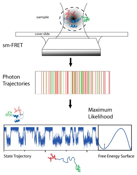
The most popular sm-FRET experiment to study protein folding has been to label a protein with donor and acceptor dyes in structurally suitable positions, and collect photons emitted by both fluorophores while the molecule is freely diffusing through the femtoliter illumination volume of a confocal microscope (two-color FRET on free diffusing molecules).⁴ sm-FRET experiments have also been performed on protein molecules immobilized on a surface (two-color FRET on immobilized molecules), which have the advantage of permitting the study of an individual molecule for times much longer than the relatively short (<1 ms) observation times of free diffusion experiments.⁴ In both types of measurements, the experimental output are sequences of photons for which the color (donor or acceptor) and arrival time to the detector are recorded with picosecond resolution. These data are commonly termed photon arrival trajectories. The major limitation in resolution for these experiments comes from the fact that observed photons are typically interspersed in intervals of several microseconds due to the inherently low detection efficiency of the confocal setup (about 1–2%) and the moderate excitation and emission rates of organic fluorophores.¹³ The standard analysis involves time binning in intervals ranging from 0.1 to 1 ms to produce histograms of averaged photon counts (photon counting histograms), which are then converted onto FRET efficiency histograms (FEHs). In these cases, FRET efficiency is simply defined as the ratio of acceptor photon counts to the total counts in each bin.¹⁴ The number of peaks in the FEH and their mean FRET values reveal molecular subpopulations and their overall structural properties as obtained from interdye distances, whereas the interchange kinetics can be obtained from their dwell time distributions.¹⁵

However, the shape of the FEH is affected by multiple factors and potential artifacts that make their quantitative analysis extremely challenging.^16,17 For instance, FRET efficiency values obtained from time bins are strongly affected by shot noise, which results from the stochastic nature of photon emission and the necessarily limited statistics afforded within a given time bin. Shot noise broadens the FEH and effectively limits the time resolution of the experiment. This is so because a minimally accurate determination of FRET efficiency requires large numbers of photons (at least 50),¹⁶ which takes long times to collect. The intrinsic conformational dynamics of the molecular process under study can also induce severe FEH distortions when the time scales for such dynamics are comparable to the binning times used in the analysis.¹⁷ In such a case, the probability that the molecule transitions between states or species during the measurement is significant, producing a dynamically averaged FEH in a phenomenon equivalent to NMR line broadening. FEHs obtained in real experiments are further distorted by the appearance of photochemical artifacts arising from transient blinking and bleaching of the fluorophores.¹⁸ Moreover, free diffusion experiments introduce further complexity in FEH analysis, since both burst time and collection efficiency vary from event to event depending on the specific translational diffusive path taken by each molecule through the confocal volume.¹⁹

Accordingly, significant efforts have been made during the last years to improve the quantitative analysis of FEH using either empirical approaches^15,20−22 or theory.^16,17,23 Parallel efforts have been undertaken to improve the time resolution of the sm-FRET technique, which is primarily limited by the number of photons emitted by the fluorophores and how efficiently they can be detected.²⁴ A major factor limiting emission rates of organic fluorophores comes from the same transient blinking and bleaching that distort experimental FEH. These dark states become highly prevalent at the high illumination conditions required to maximize fluorophore excitation, and thus restrict the photon outputs to values well below the theoretical limit. However, recent developments using purposely designed cocktails for dye photoprotection under high illumination have shown up to 40-fold increases in photon output of organic fluorophores.²⁵ The novel photoprotection methods together with instrumentation improvements that increase detection efficiency²⁶ have made it possible to reach single molecule photon detection rates of up to ∼1000 ms^–1.²⁵

All those recent developments notwithstanding, the intrinsic limitations of FEH make it difficult to extract accurate population distributions and biomolecular conformational dynamics from time binned sm-FRET data. The need for FEH alternatives is particularly pressing for fast protein folding in which the biomolecule navigates topographically complex energy landscapes by sampling different conformations in microsecond time scales. In particular, there is now a growing catalogue of single domain proteins identified as capable of folding to completion in just a few microseconds.²⁷ Fast-folding proteins are particularly attractive targets for sm-FRET experiments because their folding free energy surface is expected to be downhill or nearly downhill.²⁸ For downhill folding proteins, the subensembles of partially unfolded conformations that are typically too unstable to be experimentally detected (including the transition state ensemble) become significantly populated, permitting in principle the direct analysis of their structural properties and interconversion dynamics.⁹ Moreover, the microsecond folding kinetics of these proteins facilitate observing multiple folding–unfolding events during the relatively short (<1 ms) observation times of free diffusion sm-FRET experiments, which are less intrusive than the current procedures for immobilizing protein molecules on a surface. Along these lines, recent free diffusion sm-FRET studies with the best currently attainable photon count rates could resolve the conformational kinetics of the ultrafast-folder protein BBL (which was slowed down to ∼1/(200 μs) by performing the experiments at low temperature) but also showed that the shortest possible time bins still produced FEH with large contributions from dynamic averaging and photochemical artifacts.⁹

One alternative to FEH is to directly analyze the time stamped photon trajectories using methods based on maximum likelihood analysis. Many such methods have been in fact developed and successfully applied for characterizing various biological processes.²⁹⁻³⁶ Some of these methods use hidden Markov models (HMMs),^33,37,38 which still involve binning or converting the photon trajectories into FRET efficiency trajectories, and thus still suffer from inherent drawbacks related to low time resolution and statistical inaccuracies in converting sparse photon trajectories into FRET efficiency trajectories. The application of the HMM methods to free diffusion experiments is also nontrivial because the molecular transitions are mixed with the fluctuations in photon emission rates that arise from the stochastic nature of the diffusing trajectories.³⁹ Such complexity tends to be ignored by simply making the assumption that photon emission rates are independent of the translational diffusion of the molecule.¹⁹ To circumvent some of these problems, Gopich and Szabo developed a rigorous maximum likelihood analysis of photon trajectories (GS-MLA) that does not require binning, and which should be equally applicable for immobilized and free diffusion two-color sm-FRET experiments.⁴⁰ The GS-MLA method involves analyzing each trajectory photon by photon to compute the likelihood that the observed photon trajectory is explained by a given set of rate equations. An algorithm is then applied for data fitting to find out which rate coefficients maximize the overall likelihood for a given data set. For simple kinetic models such as a two-state process, the likelihood analysis provides an exact solution. This method has been successfully applied for extracting folding and unfolding rate coefficients from experimental single molecule measurements for the protein domains α₃D³⁴ and villin subdomain.⁴¹ An even more exciting development was the application of this method for estimating the upper bounds for folding transition path times.^10,11 The main limitation of the analysis, however, is that it is model dependent; that is, a given kinetic model must be chosen a priori, and thus, the accuracy of the results depends on how closely the molecular process under examination adheres to the kinetic model selected for the analysis. So far, the application of GS-MLA has been circumscribed to extracting elementary rate coefficients from chemical kinetic models such as the two-state and three-state models.^24,40

In this work, we extend the GS-MLA of photon trajectories to more complex kinetic models with the ultimate goal of applying it to the analysis of the conformational dynamics and general topographic features of fast-folding free energy landscapes. The idea is to employ a kinetic model that captures most of the physics of protein folding yet is simple enough to permit its direct implementation with the GS-MLA. This implies that the dynamics and shape of the free energy surface must be defined by a minimal number of parameters (ideally similar to the those required for a two-state model). The model must also be able to accommodate a variety of scenarios ranging from highly activated two-state folding all the way down to the one-state downhill folding scenario. To this end, we decided to use a simple mean-field statistical mechanical model of protein folding that was developed in our lab and which we have widely used for the quantitative analysis of protein folding experiments.⁴² The model, which is grounded on energy landscape theory,⁴³ describes folding as diffusion on a one-dimensional free energy surface (1D-FES) that represents the projection of the hyper-dimensional energy landscape of the protein into a single order parameter. In spite of its simplicity, the 1D-FES model has proven to be an extremely powerful tool for the quantitative analysis of protein folding experiments. Its successes include explaining the systematic deviations from conventional two-state behavior that are observed in fast-folding proteins,⁴² accounting for size-scaling of protein folding rates,⁴⁴ unfolding rates and protein stability,⁴⁵ the estimation of thermodynamic folding free energy barriers from the analysis of differential scanning calorimetry (DSC) experiments,⁴⁶ and the accurate prediction of protein folding and unfolding rates using size and structural class as the only input information.⁴⁷ The 1D-FES model has also been used before for the interpretation of sm-FRET data.⁹

We thus combine GS-MLA with a conveniently discretized version of the 1D-FES model (101 microstates) in which the overall shape and dimensions of the free energy surface are defined by only two thermodynamic parameters,⁴⁷ and the diffusive kinetics are described using a rate matrix formalism and a constant expression for the diffusion coefficient.⁴² As a first step, we use the 1D-FES model to perform a series of simulations of the output of sm-FRET experiments on fast-folding proteins under different scenarios (i.e., two-state folding, folding over a marginal free energy barrier, and one-state downhill folding). The results from these simulations highlight the limitations of the FEH analysis and provide a synthetic data set that allows us to investigate the performance of the GS-MLA on data for which the answer is known a priori. We then investigate the performance of the GS-MLA in retrieving the original model parameters from the synthetically generated sm-FRET trajectories as a function of typical experimental variables such as the total number of collected photons, the interphoton time, and the level of background noise.

Theoretical Model and Calculations

In this section, we provide the general implementation of GS-MLA in combination with a kinetic treatment based on diffusion on a one-dimensional potential of mean force for the direct analysis of single molecule photon arrival trajectories. We also describe the characteristics of the specific 1D-FES model that we use to represent the kinetics of protein folding and the stochastic kinetic methods for generating single molecular trajectories and photon arrival trajectories that will serve to test the method’s performance.

Conformational Dynamics as Diffusion on a Free Energy Surface

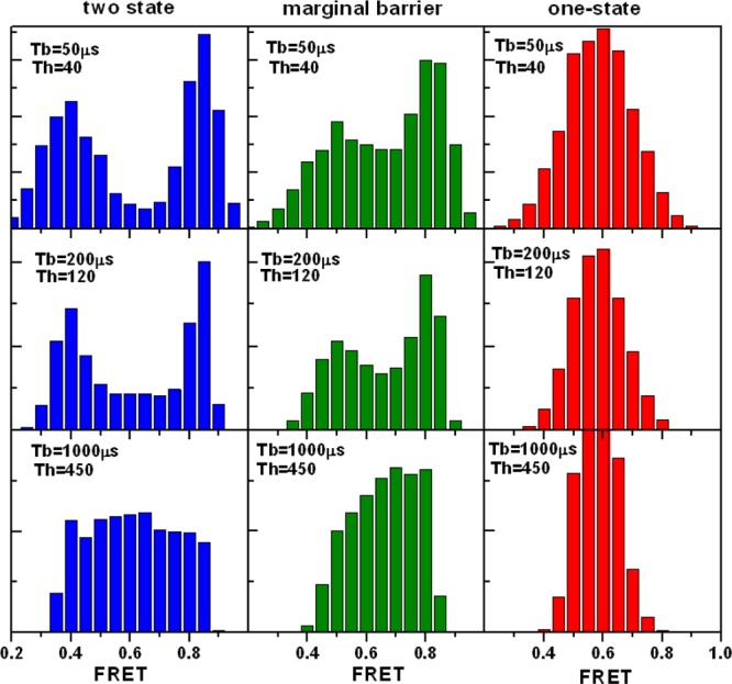
We describe the kinetics of protein folding as diffusion on a potential of mean force defined as a function of a single reaction coordinate, r (i.e., V(r)). By discretizing the potential of mean force into a set of defined species, it becomes possible to effectively describe the diffusive kinetics of the system with the rate matrix⁴⁸

1

where k_i,i+1 = (1/2)D((p_i/p_i+1) + 1) and k_i,i–1 = (1/2)D((p_i/p_i–1) + 1) are the diffusive rates for converting species i into the next and the previous species along the reaction coordinate, respectively. D is the intramolecular diffusion coefficient that determines the time scale of the dynamics, and p_i is the probability of microstate i, which is defined as

2

in which n is the number of discrete species at fixed intervals over r. K can be diagonalized to obtain the Eigen spectrum from which the relaxation rate is directly obtained. Here we apply this treatment to protein folding kinetics in which the potential of mean force is a one-dimensional free energy surface as a function of the order parameter nativeness (see below). However, it is important to emphasize that the method is directly applicable to any other molecular process that can be described in terms of diffusion on a 1D potential of mean force V(r).

Maximum Likelihood Method for Analyzing Photon Trajectories

For a photon trajectory with N photons from a freely diffusing molecule (or a trajectory from an immobilized molecule), the likelihood that it arises from the conformational dynamics and set of interdye distances determined by the rate matrix K is given by

3

F(acceptor) = E and F(donor) = I – E, where I is the identity matrix and E is a diagonal matrix of FRET efficiencies for the microstates (ε_i). p_eq is a vector defining the equilibrium probabilities; τ_j is the interphoton arrival time between the j – 1th and jth photon; c₁ is the color of the first photon in the trajectory (i.e., whether it is an acceptor or donor); and c_j is the color of the jth photon. After N successive matrix-vector multiplications, a final multiplication by the identity column vector (1^T) sums the product over all conformational states to yield the likelihood L_t. For multiple bursts (different photon trajectories), the total likelihood is obtained from ln L = ∑_t ln L_t, which avoids computer precision overflow due to the extremely small numbers involved in the likelihoods of each photon trajectory. The most likely parameters defining the potential of mean force and the conformational dynamics (D) are those that maximize the total likelihood. The rate matrix K can be used in diagonalized form to speed up calculations, as described in ref (40).

1D Free Energy Surface Model for Protein Folding

For all the calculations discussed in this work, we used a simple 1D-FES model of protein folding that has been described in detail before.^42,47 Briefly, this model calculates a one-dimensional free energy surface as a function of a single order parameter termed nativeness (n), which represents the average probability that any protein residue resides in its native dihedral angle values (thus n ranges from 1 for the native state to 0 for the completely unfolded state). The model has terms for entropic and enthalpic contributions that scale linearly with the number of residues (N) in the protein, and which are defined as functions of the order parameter as follows

4

5

6

where N is the number of residues in the protein and ΔS_res is the entropy cost of fixing a residue in its native conformation. For all calculations, ΔS_res was set to a constant value of 16.5 J mol^–1 K^–1 that corresponds to the average empirical estimate obtained from a collection of DSC data,⁴⁹ as it was done before.⁴⁷ We define the stabilization enthalpy (ΔH^total(n)) as the sum of two Markov processes, one that corresponds to the formation and breakage of stabilizing local interactions (interactions between residues separated in the chain by four or fewer residues) and another one that corresponds to the formation and breakage of nonlocal interactions.⁴⁷x is the characteristic Markov constant for breaking native interactions, and the quotient [(1 – x^(1–n))/(1 – x)] gives the fraction of the native stabilization energy that remains at any given value of n. As before,⁴⁷ the rate for local interactions is set to a high value (x_local = 3.5), resulting in a shallow increase in energy from the native state. The rate for nonlocal interactions is set to a low value (x_non-loc = 0.002), resulting in a steep increase in energy as n decreases from the native state (as the protein unfolds). The balance between enthalpy and entropy renders the free energy as a function of n (ΔG(n)). The resulting free energy surface exhibits two minima at values of nativeness near 1 (native state) and between 0.2 and 0.5 (unfolded state) separated by a barrier that arises from the incomplete compensation between the decreasing entropy and stabilization enthalpy functions. Therefore, the barrier height is ultimately determined by the curvature of the stabilization enthalpy, which is defined by the ratio between the contributions from the local and nonlocal enthalpy terms (i.e., the lower the ratio the higher the barrier). The values for the curvature of the local and nonlocal stabilization enthalpy functions employed in this work correspond to the average values obtained previously from fitting the kinetics of an experimental data set of 52 proteins.⁴⁷ Therefore, the shape of the 1D free energy surface of a given protein is entirely defined by the magnitudes of ΔH_local,res and ΔH_nonlocal,res, which vary from protein to protein, thus encompassing all possible folding scenarios.

Simulating Folding Scenarios with the 1D-FES Model

For the calculations described in this work, we chose specific parameters for the 1D-FES model that define three potentially feasible scenarios for a fast-folding protein: (1) two-state-like folding scenario in which the native and unfolded states are separated by a significant barrier of ∼4 RT; (2) marginal barrier scenario in which the two states are separated by a minimal barrier that amounts to only 1 RT at the denaturation midpoint; (3) one-state downhill scenario in which the 1D-FES only has one minimum that shifts from native to unfolded values as the denaturation stress (e.g., temperature) increases. The specific parameters used for simulating the three scenarios are given in Table 1. Folding kinetics were described as diffusion on the 1D-FES using ΔG(n) as defined in eq 6 to replace the potential of mean force from eq 2. Practically, for the calculations presented here, we defined 101 microstates at even intervals of n between 0 and 1. For the sake of comparison, the simulations performed in this work were all carried out choosing D values for the three scenarios scaled to result on the same overall relaxation kinetics with τ ≈ 200 μs regardless of the shape of the free energy surface (see Table 1).

Table 1. Results from the Analysis of the Three Folding Scenarios Using the Combination of the 1FES Model and MLA Procedure Described in the Theoretical Model and Calculations Section^a.

	ΔHloc,res (kJ/mol)		ΔHnonloc,res (kJ/mol)		log(D)
scenarios	real	recovered	real	recovered	real	recovered
two-state	2.70	2.69 ± 0.019	3.81	3.81 ± 0.012	7.00	6.99 ± 0.030
marginal barrier	3.72	3.72 ± 0.034	3.36	3.35 ± 0.014	6.31	6.32 ± 0.025
one-state downhill	5.42	5.49 ± 0.120	2.31	2.26 ± 0.080	5.51	5.49 ± 0.016

^aRecovered parameters were obtained after applying the MLA procedure to packets of 100 000 photons from trajectories simulated at a count rate of 800 ms^–1. The reported errors are the standard deviation from the set of parameters obtained for 50 different trials.

Stochastic Simulations of Conformational Transitions and Photon Emissions

Using the rate matrix (eq 1) defined by introducing the 1D-FES model into eq 2, we performed stochastic kinetic simulations of the conformational dynamics of an individual molecule as it diffuses on the 1D-FES. In addition, we implemented in the simulations the possibility of the molecule emitting donor or acceptor photons according to the FRET efficiency of each of the 101 microstates included in the rate matrix. To perform these stochastic kinetic simulations, we employed a procedure similar to the original Gillespie algorithm.⁵⁰ In particular, we defined four possible events that can take place in the molecule after a given time step Δt:

• -emission of one acceptor photon (with time probability defined by count rate n_Ai)
• -emission of one donor photon (with time probability defined by count rate n_Di)
• -transition from i to i + 1 (with time probability defined by k_i,i+1)
• -transition from i to i – 1 (with time probability defined by k_i,i–1)

For the molecule in state i, the photon emission rates are Poissonian and specified by the count rates (n_Ai or n_Di). The time intervals (Δt) between successive events are generated by randomly drawing values from an exponential distribution, exp(1/k_T), in which k_T is the sum of the rates for all possible events that can occur at any given time: k_T = n_Ai + n_Di + k_i,i+1 + k_i,i–1. The particular events taking place at those times are randomly picked according to the probabilities given by [n_Ai, n_Di, k_i,i+1, k_i,i−1]/k_T. The elementary rate constants for the transitions are taken from the rate matrix, and the initial state is chosen randomly according to the equilibrium probability vector p₀. Acceptor and donor count rates for each state i are obtained by multiplying the total count rate (which here we set to 800 photons per millisecond) by the FRET efficiency of the species (ε_i). For the purpose of fitting experimental data, ε_i can be defined using a linear mapping with nativeness according to the expression ε_i = R₀⁶/(R₀⁶ + r(n)⁶), where r(n) = r_u – n(i)Δr. Here R₀ is the known Forster radius for the given FRET dye pairs, r_u is the end to end distance in the fully unfolded state, and Δr defines the decrease in end to end distance as a function of nativeness. This mapping requires two additional parameters (R₀ is a constant that depends on the donor and acceptor pair), which in practice can be set a priori based on the FRET efficiencies observed in FEH at extreme concentrations of denaturant. For simplicity, in the simulations we performed here we assumed that the FRET efficiency of a given species is identical to its nativeness (ε_i = n_i). The output from the simulations is a state trajectory containing the changes in microstate of the molecule plus the strips of donor and acceptor photons emitted stochastically as a function of the given count rates (photon trajectories). Varying the number of steps in the simulations, we could easily obtain state and photon trajectories of different duration. In particular, we calculated very long trajectories that were chopped into small fragments of 1000 photons (∼1.25 ms) for analysis. To simulate FEH from free diffusion experiments, we produce a distribution of photon bursts by generating random fragments of the state trajectory according to an exponential distribution with a characteristic time of 1 ms (i.e., the mean diffusion time across the confocal volume).

Maximum Likelihood Analysis of Simulated Photon Arrival Trajectories

In terms of the number of parameters, the 1D-FES is not significantly more complex than previous implementations of the GS-MLA that used simple two- or three-state chemical models.³⁴ This is so because the shape of the 1D-FES is completely specified by two parameters (local and nonlocal enthalpies per residue) and the conformational dynamics by just one (the intramolecular diffusion coefficient D). However, from a numerical standpoint, calculations with the 101 × 101 rate equation of the 1D-FES model are much more involved than previous implementations using 2 × 2 or 3 × 3 rate matrices. To speed up calculations, we diagonalized the rate matrix once for each set of parameters explored during the fitting procedure and then performed the likelihood calculations with eq 3 implemented with the diagonalized rate matrix. In adition, we devised a two-step procedure for parameter search during data fitting in which we first defined an extensive grid in parameter space to identify the overall region where the global minimum is located. Once the area for the global minimum was identified, we fine-tuned the parameters using an intensive optimization with the simplex algorithm (as implemented in the fminsearch function in Matlab (Mathworks Inc., USA) starting from the grid point that rendered the maximum likelihood value).

Results and Discussion

Stochastic Kinetic Simulations of sm-FRET Experiments on Fast-Folding Proteins

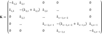
To sample the range of mechanistic scenarios available to fast-folding proteins, we chose three particular examples that correspond to (1) two-state-like folding (i.e., folding over a free energy barrier >4 RT at the denaturation midpoint); (2) marginal downhill folding (i.e., crossing a minimal free energy barrier of ∼1 RT at the denaturation midpoint); and (3) one-state (global) downhill folding (i.e., free energy surface with a single minimum at the denaturation midpoint). Using the 1D-FES model and choosing a protein domain of 50 residues as a model, we could generate these three basic folding scenarios with moderate differences in the two basic parameters that define the FES shape (ΔH_loc,res and ΔH_nonloc,res) (see Table 1). We then set D for each folding scenario so that the folding dynamics is the same for all of them and corresponds to an overall relaxation rate of 1/(200 μs). The resulting 1D-FES and probability distributions at the denaturation midpoint are shown in Figure 1.

Figure 1.

1D free energy profiles and probability distributions for the three folding scenarios.

The three combined scenarios nicely reproduce the gradual shift in the position of the native and unfolded ensembles as a function of the height of the folding free energy barrier that has been observed experimentally.⁴² This trend results in the progressive merging of both minima with an unfolded state with increasing residual structure as the barrier becomes smaller and a native state that simultaneously becomes more unstructured (Figure 1). We then performed stochastic kinetic simulations of the three scenarios to generate single molecule conformational state trajectories and photon trajectories as described in the Theoretical Model and Calculations section. For these simulations, we used a photon count rate of 800 ms^–1, which is close to the maximum limit currently attainable from sm-FRET experiments using organic fluorophores,²⁵ and did not consider the effects of photochemical artifacts. Therefore, the simulated photon trajectories that we generate represent an experimental scenario that is nearly optimal given current technical limitations. The left column of Figure 2 shows the stochastically generated equilibrium conformational distributions with a total simulation time of 20 s for each scenario. These conformational distributions have excellent agreement with the analytical probability distributions from the model (Figure 1), indicating that 20 s is sufficient sampling time for these systems. The central column in Figure 2 shows a 25 ms fragment of conformational state trajectory for illustration of the differences in single molecule behavior produced by the three scenarios. The differences in single molecule behavior among the three scenarios are highly noticeable even though the simulations have been performed keeping the overall relaxation rate constant. In these conformational state trajectories, the two-state-like scenario produces the typical pattern of switching between a native state with low structural fluctuations (i.e., state values close to 100, or n ∼ 1) and an unfolded state in which the structural excursions are of higher amplitude (i.e., state values close to 40, or n ∼ 0.4). The trajectory for the marginal barrier scenario produces a similar switching pattern to a first approximation, even though the free energy barrier is in this case minimal (i.e., equivalent to thermal energy). Close inspection of the trajectory (green in Figure 2), however, reveals events in which the molecule visits the barrier top from either one of the two FES minima, then stays at the top for a significant fraction of time (for this scenario, the population of the barrier top is significant, see Figure 1), and then returns back to the originating minimum (e.g., event occurring at 0.205 s in the green state trajectory of Figure 2). This is an interesting observation because such single molecule behavior, which in this case is characteristic of a highly populated transition state ensemble, could be easily confused with the formation of a folding intermediate. In contrast, the one-state downhill folding scenario produces notoriously distinct state trajectories that closely resemble the Brownian dynamics on a harmonic well. Finally, the right column of Figure 2 shows examples of short photon trajectories for the three scenarios.

Figure 2.

Stochastic kinetic simulations of the three fast-folding scenarios. The left column shows the conformational distributions obtained after sampling for 20 s. The central column shows examples of 25 ms state trajectories in which the y axis represents the index for each species in the model (i.e., species 1 corresponds to n = 0 and species 101 to n = 1). The right column shows examples of short photon trajectories.

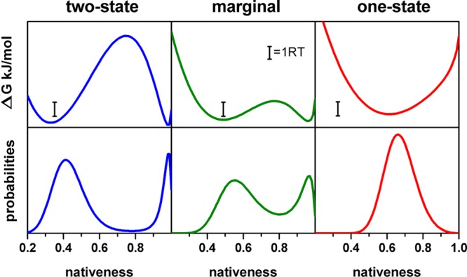
The photon trajectories simulated for the three folding scenarios give us the opportunity to evaluate the limitations of binning photon data for the analysis of fast-folding proteins with microsecond conformational dynamics. The results from such an analysis are summarized in Figure 3, which shows the simulated FEH calculated with different binning times for the three scenarios employing a collection of photon trajectories (50 000 per scenario) with exponentially distributed times to mimic the output of typical free diffusion experiments. The very high photon count rates (800 ms^–1) and the moderately fast-folding rate (1/(200 μs)) that we have used in these simulations allow us to assess the top performance that is currently feasible for binning methods. For example, calculating the FEH from these data using a conventional binning time of 1 ms allows greatly reducing shot noise because under these conditions the photon threshold can be raised up to 450 photons. However, the obtained FEH are highly distorted even in the absence of photochemical artifacts (not included in this analysis) because the binning time is long relative to the molecular relaxation, which results in high contributions from dynamic averaging. Thus, all of the FEHs become essentially unimodal and featureless, so that determining whether the underlying scenario is truly one-state or has two states separated by a barrier becomes impossible (bottom of Figure 3). Decreasing the binning time to times equivalent to the molecular relaxation still affords the use of fairly high photon thresholds (i.e., 125) to minimize shot noise, and results in FEHs that now show two peaks for the two-state and marginal barrier scenarios and a unimodal distribution for the one-state downhill folding case (middle of Figure 3). However, the 0.2 ms FEHs are still plagued by large contributions from dynamic averaging that make it extremely challenging to distinguish between the two-state and marginal barrier scenarios. Finally, calculating the FEH with the shortest possible binning times that still afford reasonable photon thresholds, which in this case implies using a binning time of 50 μs (4-fold shorter than the molecular relaxation) and a photon threshold of 40, produces clearly bimodal distributions for the two-state and marginal barrier scenarios, and a distinctly unimodal distribution for one-state downhill. In this limiting case, dynamic averaging is minimized at the expense of shot noise. Such a trade-off seems to be sufficient to identify the one-state downhill scenario, as it has been reported experimentally for the fast-folder protein BBL.⁹ However, distinguishing between the two-state and marginal barrier scenarios remains challenging because the FEH resulting from the marginal barrier case is very similar to that of a two-state scenario with some degree of dynamic averaging. Moreover, in real experiments, such small differences in FEH would be easily masked by the presence of even low levels of photobleaching and blinking.

Figure 3.

Sample (100 μs) FRET efficiency histograms (FEHs) obtained with binning times of 50, 200, and 1000 μs and photon thresholds of 40, 120, and 450, respectively. FEHs were calculated using simulated data corresponding to 50 000 bursts assuming that the average residence time of the molecule on the confocal volume was 250 μs.

We can thus conclude that with the inherent technical limitations of current sm-FRET experiments it is not possible to resolve the shape of folding free energy landscapes or the height of the free energy barrier for fast-folding proteins using conventional photon binning approaches.

Maximum Likelihood Analysis of Simulated Photon Trajectories

In parallel, we used the simulated data for the three folding scenarios described above to assess the performance of MLA methods in extracting mechanistic information from complex sm-FRET data. Particularly, the goal is to determine whether the GS-MLA procedure could accurately retrieve the original free energy surface and diffusion coefficient for our three folding scenarios utilizing data limited in time resolution (count rate) and in total photon numbers. This is of course possible in this case because as input we use synthetic data for which the model parameters are known a priori. The results from this analysis are shown in Table 1. To better assess performance and accuracy of the procedure, we performed the GS-MLA analysis combined with the 1D-FES model 50 different times for each folding scenario, using a different packet of 100 000 photons (a different input set of 125 1 ms long trajectories) for each run. We obtained optimal model parameters by carrying out an automatic optimization protocol in two steps. The first step consisted of performing a coarse-grained analysis of the global parameter space by calculating the ML over a multidimensional parameter grid. In the second step, we picked the parameters corresponding to the grid point with the highest likelihood and performed further local optimization using a simplex algorithm. Overall, we observed that such an optimization protocol was able to retrieve the original parameters for the 1D-FES model with high accuracy and reproducibility (see Table 1). This was the case for the three folding scenarios in general. Interestingly, the presence of a free energy barrier separating the native and unfolded states, no matter how small (i.e., 1RT for the marginal barrier scenario), seemed to increase the accuracy and reliability of the parameters that define the free energy surface (ΔH_local,res and ΔH_nonlocal,res). Beyond the general accuracy of the method in retrieving the parameter values for the folding scenarios containing a barrier, it is noteworthy that the small discrepancies in retrieved parameters do not alter the FES shape and the height of the resulting free energy barrier in any significant way (e.g., the error in barrier height is less than 0.15 kJ/mol). Presumably, the excellent performance stems from the linear mapping that exists between changes in the two parameters defining the FES and the height of the resulting barrier when there is actually one. The accuracy of the retrieved parameters for the one-state downhill case is somewhat poorer although still high (see Table 1). Moreover, such parameter differences do not affect the overall FES shape, which is systematically concave with a single minimum, and thus consistent with one-state downhill folding. Further inspection of the results indicated that the larger spread in retrieved parameters that we observed for this scenario results from the more complex mapping between parameters and FES shape that emerges once the free energy barrier vanishes (i.e., multiple combinations of parameters produce very similar concave FES). Interestingly, the GS-MLA procedure proves to be equally powerful in obtaining direct dynamical information from the photon trajectories. Such a statement is demonstrated by the very low error in the retrieved values of the diffusion coefficient for the three scenarios (see Table 1). The GS-MLA approach is, therefore, capable of simultaneously extracting the static conformational distribution and the overall dynamics for the three scenarios even though the time scales are significantly different (i.e., the global relaxation rate is set to be identical by compensating free energy barrier differences among scenarios via changes in the diffusion coefficient). The implication is that the GS-MLA procedure is able to resolve the details and time scales of the underlying state trajectories from apparently featureless stochastic strips of photons (e.g., see the right column of Figure 2). Such performance is remarkable given the highly demanding nature of this test. The GS-MLA procedure has been previously utilized in conjunction with simple two- or three-state chemical models in which the molecular behavior is reduced to discrete transitions described by global rate coefficients. Here, however, the intrinsic complexity of the state trajectories is much higher because the molecule visits about a hundred different microstates with widely different populations. Moreover, whereas the interphoton time in our simulations is much shorter than the overall folding relaxation, during the ∼1.25 μs average interval between photons (count rate of 800 ms^–1), the molecules typically undertake multiple transitions between microstates; e.g., for the two-state scenario, 10 transitions between next neighbors occur in only 1 μs.

Summarizing, in our simulations, the GS-MLA procedure seems to pick up dynamic processes that are even faster than the interphoton time. From a practical standpoint, this characteristic of the GS-MLA may prove useful for increasing the effective time resolution of sm-FRET experiments. We should not forget that the performance tests described in this section have simulated idealized experimental conditions. In real experiments, however, there are many different factors that affect the quality and accuracy of sm-FRET data. For example, the number of single molecule bursts that is available and their time duration could be limited; sustainable count rates are oftentimes lower than 800 ms^–1; and recorded photon trajectories come inevitably with contributions from background counts from both the donor and acceptor channels. In the next sections, we investigate the sensitivity of the GS-MLA combined with the 1D-FES model to each of these experimental factors as a means to characterize the applicability limits of the method over a broad range of conditions.

Dependence of MLA Performance on Sample Size

Like for any other statistical inference procedure, the results produced by MLA depend heavily on the amount of input data. The sample size determines how closely the observed data reproduces the parent distribution. When implemented with a two- or three-state model, the MLA is only required to count two or three species and their transition frequencies, a task that does not require large numbers of photons. Using the 1D-FES model is much more challenging because this model includes over 100 microstates that exchange with their neighbors in time scales much shorter than the global relaxation process. It is thus key to determine what amounts of input data does the MLA require for accurately capturing the FES shape and conformational dynamics. We tested this question by performing the MLA procedure with input data varying from a maximum of 100 000 photons (as used in the previous section) down to 5000, the latter corresponding to only 6.25 ms of state trajectory time at a count rate of 800 ms^–1. The global results from this exercise are summarized in Figure 4, which plots the deviations in the probability and diffusion coefficient retrieved by the MLA relative to the input simulated data for the three folding scenarios. Figure 4 shows an almost invariant MLA performance for retrieving the probability distribution and conformational dynamics as long as the sample includes 20 000 photons or more (25 ms of molecular trajectory, which is equivalent to the trajectories shown in Figure 2). When the input data decreases from the 20 000 photons threshold, MLA performance degrades considerably, producing noticeable differences between the retrieved FES and D and the actual input data. These differences, however, do not seem to be caused by worsened MLA performance but by poor overall statistical sampling. This factor is best appreciated in Figure 5, which shows the probability distribution retrieved by MLA from various statistical samples in comparison with the parent distribution (calculated with the original parameters) and also with the histogram of the actual input data. Figure 5 confirms the excellent MLA performance when it is fed with 100 000 photons worth of data (or 125 ms of molecular trajectory). As input photons decrease, the retrieved distribution progressively diverges from the parent distribution. For 10 000 photons, the differences between the two distributions are already quite apparent (left in Figure 5).

Figure 4.

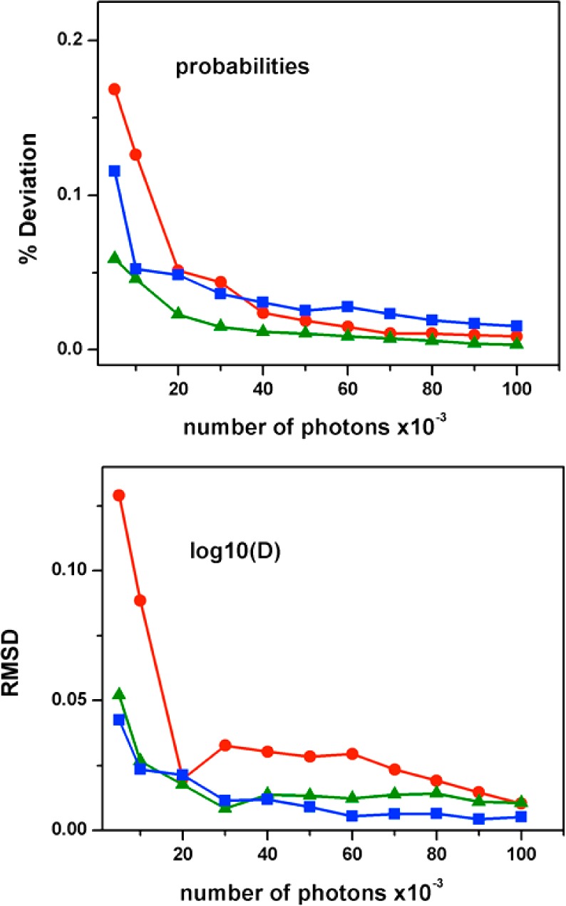
Performance of MLA as a function of sample size. Panel A shows the difference between the probability distribution recovered by MLA and the normalized input data from stochastic simulations in percentage. Panel B shows the root-mean-square deviation between the log(D) recovered by MLA and the original log(D) used in the stochastic simulations. The color code is the same as that in previous figures: blue, two-state; green, marginal barrier; red, one-state downhill.

Figure 5.

Dependence of the MLA performance on the amount of input data. The recovered probabilities, the parent distribution, and the normalized counts of the input simulations are shown for different amounts of data (number of photons) and each of the three scenarios.

Poor sampling makes the input data differ significantly from the parent conformational distribution (see differences between black and red lines in Figure 4), and thus, the MLA computes the 1D-FES that most closely reproduces the limited input data rather than the parent distribution. It is interesting that such deviations caused by poor sampling do not seem to significantly affect the estimated free energy barrier height or the identification of the proper folding scenario, but rather, they randomly distort the ratio between the native and unfolded ensembles. For example, the populations of species with high nativeness are overestimated for the two- and one-state scenarios and underestimated for the marginal barrier case. Therefore, we can conclude that conformational sampling is the main factor limiting the ability to determine an accurate 1D-FES using limited data. The analysis performed with 10 000 photons, which after all corresponds to only 12.5 ms of the simulated molecular trajectory, provides good local sampling (i.e., neighboring microspecies interconvert very quickly), but it is hardly sufficient to guarantee complete sampling given that the overall folding relaxation takes ∼200 μs. On the other hand, the MLA performance does not seem to be negatively impacted by the large number of molecular species that we use for defining the 1D-FES (101). The results summarized in Figures 4 and 5 indicate that the method does in fact perform quite well with inputs of only 50–100 photons per species included in the molecular model. Such performance is possibly highly enhanced relative to what would be expected from chemical models because the 1D-FES model is entirely defined by three global parameters, whereas linear chemical models require at least two new parameters for each additional species. In general, the combination of the 1D-FES model and GS-MLA procedure appears to provide an extremely robust tool for the analysis of limited photon trajectory data.

Testing for Dynamic Effects by Altering the Photon Count Rate

The tests performed in the previous sections use count rates that correspond to what is maximally achievable with current sm-FRET experiments. Another major factor in determining the performance of the GS-MLA is the sensitivity of the procedure to the interphoton time relative to the conformational dynamics of the system under study. This is a critical parameter to determine whether the resolution of the procedure is determined by the local dynamics time scale or by the global relaxation. Although in this work we are mostly interested in the analysis of fast-folding experiments, such dynamic information is extremely useful in general, as it sheds light onto the absolute limits in time resolution for MLA based on photon trajectories as opposed to conventional photon binning. The analysis of dynamic performance is also complementary to that described in the previous section, as we can investigate the change in MLA performance as the time intervals between photons increase while the total number of input photons (or alternatively the total simulation time) is kept constant. Moreover, it is also a key test for identifying the minimal count rates that still resolve the dynamics of the process under study so that experimentalists can decide to lower the illumination intensity to trade noncritical time resolution for improved photochemical stability of the dyes.

For these tests, we varied the photon count rate from 800 down to only 10 ms^–1 (equivalent to conditions of very high photostability) while we kept the total number of photons used for MLA fixed. One potential caveat in this analysis is how to correct for statistical sampling effects from the viewpoint of the duration of the molecular trajectory. As count rates decrease, it obviously takes a much longer time to measure the same total number of photons, which makes the molecular trajectory concomitantly longer. To minimize this problem, we carried the test setting the number of photons to 100 000, which, as we know from our previous tests (see above), affords a sufficient molecular trajectory to minimize sampling problems at the maximal count rate of 800 ms^–1. The longer molecular simulations required to test for lower count rates will thus not show significant statistical improvements given that adequate sampling is already guaranteed for all conditions. The parameter that is most relevant for testing the dependence on the interphoton time is the intramolecular diffusion coefficient, which defines the overall time scale of motion along the 1D-FES, and thus the rate of conformational exchange. In these tests, we are more interested in the relative time resolution, which is easily generalizable for any other experimental condition and/or molecular system, than the absolute time resolution. Therefore, as a relevant dynamic parameter, we use the relative interphoton time defined as the average time interval between photons (set by the count rate) divided by the global relaxation time of the process under study (here set to 200 μs for the three scenarios). Figure 6 shows the results from such tests by plotting the same two parameters used above (percentage difference in probability and RMSD of log(D)) as indicators of overall performance. The test results are quite remarkable because they show that MLA performance is virtually insensitive to the photon count rate over a broad range that reaches a minimum of only 10 photons per relaxation, which in this case is equivalent to measuring only one photon every 20 μs or a count rate of 50 ms^–1. Figure 6 indicates that the MLA of photon trajectories affords a 20-fold increase in time resolution relative to conventional photon binning approaches (see Figure 3), which practically means that a count rate of 800 ms^–1 may be sufficient to resolve dynamics processes that take place in just 10 μs using sm-FRET experiments. Here the results that are most informative are for the one-state downhill scenario because in this case the conformational dynamics are entirely diffusive and do not involve barrier crossing events. Along these lines, our results indicate that the MLA procedure can pick up the correct underlying molecular dynamics even if there is enough time for the system to undergo an average of three local transitions during the time interval between detecting two photons (we set D to ∼300 000 s^–1 for one-state downhill; see Table 1). Past this limit, one must be cautious because the performance appears to degrade rather quickly when fewer than 10 photons are detected per relaxation time (Figure 6).

Figure 6.

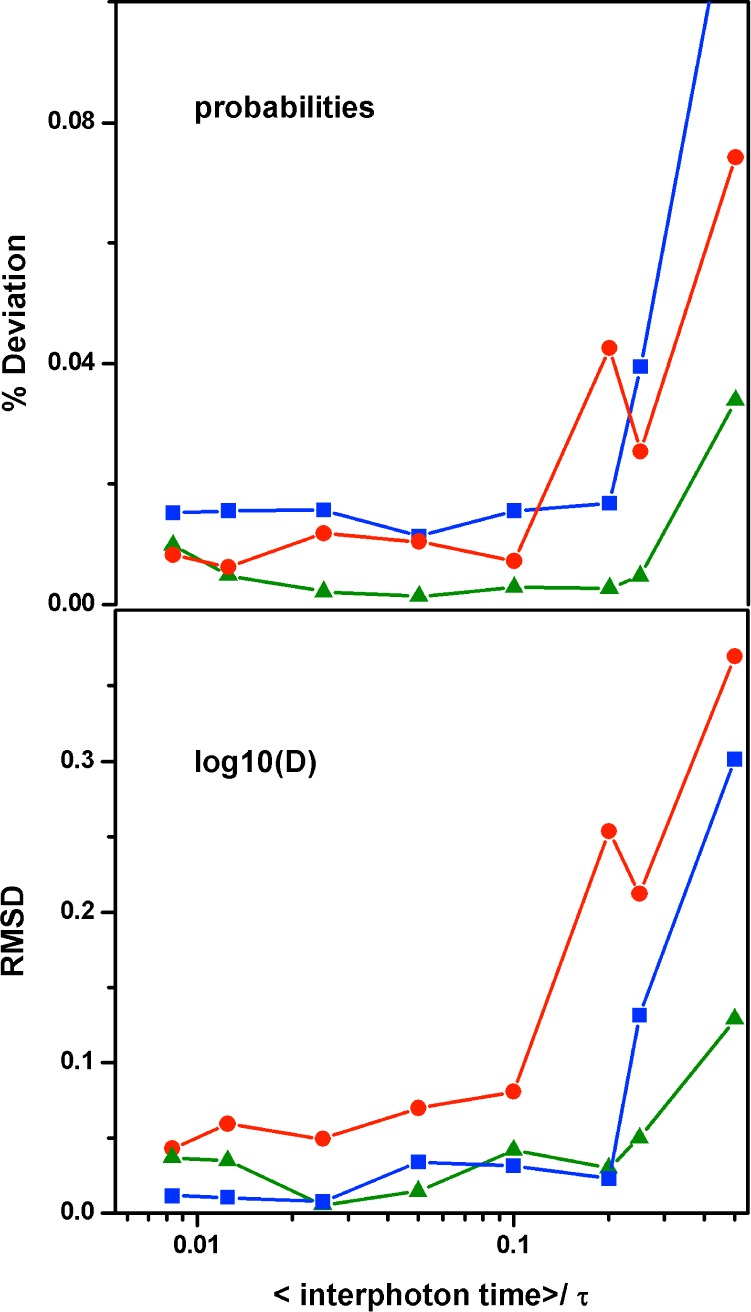
MLA performance as a function of photon count rate. (A) Percentage difference between the recovered probability and the normalized counts in the input simulations versus the ratio between the average interphoton arrival time and the molecular relaxation time (τ = 200 μs). (B) RMSD of log(D) retrieved from the MLA versus the ratio between the average interphoton arrival time and the molecular relaxation time. Color code for the three scenarios as above.

Nevertheless, this is an extremely important finding, since the GS-MLA method combined with a free energy surface model emerges as a simple way to effectively increase the time resolution of sm-FRET methods by over an order of magnitude. Practically, this means that the approach offers a solution for resolving both the conformational dynamics and folding free energy landscape of most fast-folding proteins identified to date. Our results are also consistent with the findings from the statistical analysis of folding transition paths from photon trajectories using chemical models.^10,51 Moreover, the GS-MLA approach is in principle generalizable. For instance, our procedure can be extended to any other molecular process involving microsecond dynamics (e.g., protein binding, protein catalysis, molecular motors, RNA folding) by simply replacing the underlying free energy surface model by a detailed model suited for the particular problem at hand.

Effects of Background Noise

All of the tests described in previous sections have been performed with idealized simulated data that did not include any contributions from experimental noise. True experimental data, however, contains several noise sources. Beyond photochemical artifacts, which can be somewhat controlled through the illumination intensity and addition of photoprotecting agents,²⁵ real sm-FRET data inevitably contains certain levels of background counts detected in both donor and acceptor channels. Background noise impairs the ability to convert experimentally determined FRET efficiency values into molecular distances, and can thus heavily distort the FEH, impeding its quantitative analysis. Gopich and Szabo have argued that one of the intrinsic advantages of MLA of photon trajectories relative to conventional photon binning is a high intrinsic resilience to the FRET efficiency distortions caused by background counts.⁴⁰ To test empirically the practical implications of such assertion, we performed the MLA on the three simulated folding scenarios under conditions of varying background noise. Figure 7 illustrates the effects of background noise on measured FEH using the marginal barrier scenario as an example. In this case, we simulated a rather high level of background noise (10% of the total number of recorded photons) equal for both channels. The effect of the background noise is manifested by the compression of the FRET efficiency dynamic range, resulting in a FEH in which the native and unfolded peaks are closer together and there is an apparent increase in the population of any species with intermediate FRET values (see black FEH in Figure 7). The effects of uneven background noise levels in both channels are in essence the same, the only difference being that the compression factor is accompanied by an offset in the experimentally determined FRET efficiencies. Figure 7 demonstrates that dealing appropriately with background noise is key for identifying and quantifying the population levels of rare/unstable intermediates (e.g., the species at the top of the folding free energy barrier). To account for background noise in the MLA of photon trajectories, it is necessary to implement the method with a procedure for converting measured FRET efficiencies with background noise onto true molecular FRET efficiencies. This can be achieved using the following formula

where ⟨n_t⟩ is the total count rate (i.e., the total number of detected photons per ms), b_D and b_A are the background rates in the donor and acceptor channels, and ε_i^calc is a vector containing the true molecular FRET efficiencies for all the species defined in the 1D-FES model. The total count rate and donor and acceptor background rates are easily measured in the experimental setup, so they can be empirically determined and fixed in advance. ε_i values are obtained directly by fitting during the MLA procedure. In our case, the nativeness values from the 1D-FES are converted onto ε_i^calc using the simple mapping described in previous sections. In dealing with real experimental data, ε_i values can be estimated directly from the measured FEH and the 1D-FES model applying the same formula in reverse.

Figure 7.

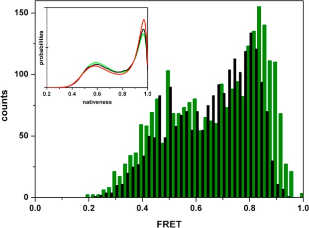
Effect of background photons on the FEH. A FEH for the marginal barrier scenario computed using the same procedure described in Figure 3, a photon threshold of 120, and a binning time of 0.2 ms is used here for illustration of the effects of background noise. (green) Histogram without background noise; (black) histogram obtained after adding 10% of random background photons to both the donor and acceptor channels. The inset shows the probability distribution recovered from the data with 10% background noise (red) relative to the input simulated data (black) and the parent probability distribution (green).

The MLA implemented with this simple procedure was able to successfully analyze the input photon trajectory data containing 10% background noise and retrieve a probability distribution that is reasonably close to both the input data and the parent distribution (inset of Figure 7). The comparison shown in the inset of Figure 7 highlights that the retrieved distribution overestimates the population of the native ensemble at the expense of the populations of the unfolded and free energy barrier ensembles. The deviations in population are not insignificant, but when converted into free energies, such discrepancies are still well below thermal energy and do not compromise the proper identification of the folding scenario or even a rather accurate estimate of the barrier height (the estimated barrier is off by only ∼0.3 RT). Moreover, 10% is a very high level of background noise. With recent instrument developments, the level of background noise in sm-FRET experiments is often below 5%.²⁴ Interestingly, MLA performance seems to be much better for more realistic background noise levels, as Figure 8 illustrates. In this figure, it can be observed that there is an abrupt deterioration in MLA performance at background noise levels above 10%, but the procedure is rather insensitive for levels below 7.5%. In contrast with the effects of sample size and count rate, background noise seems to affect one-state downhill to a lesser extent than it affects the barrier limited scenarios. This is probably so because the compression of the FRET dynamic range caused by background noise is less critical for determining a unimodal distribution. The scenario that is most affected for the determination of the probability distribution is the marginal barrier one, in which the region of intermediate FRET values has a small but still significant population. For the two-state scenario, the background noise effects tend to concentrate on the dynamic term (D), whose deviations reflect errors in the population of the species at the barrier top, which, although they might be small in absolute terms (i.e., below 1%), become very significant when converted into free energies.

Figure 8.

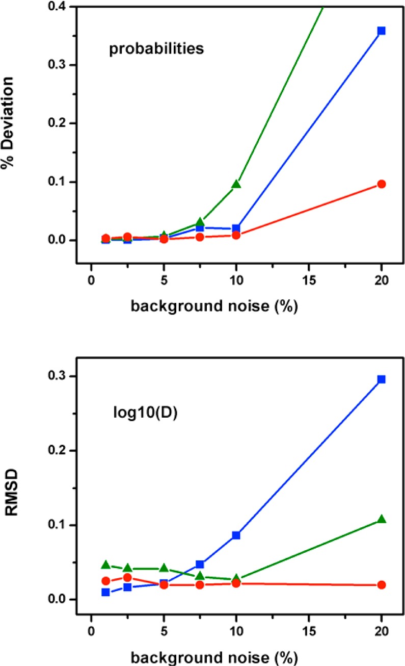
MLA performance under different amounts of background photons on both channels. (A) Percentage difference between the probabilities recovered by the procedure and the normalized input data versus the photon background level. (B) RMSD of log(D) retrieved from the MLA versus the photon background level. The photon background level is defined as the percentage of the total number of photons.

Summarizing, our analysis confirms that the MLA of photon trajectories is indeed an excellent tool for the quantitative analysis of real sm-FRET including reasonable levels of background noise. The effects on the probability distribution and folding scenario ascription are minimal. However, Figure 8 indicates that an accurate determination of the dynamic term and the free energy barrier height for a two-state folding scenario requires that the background noise level is kept below 7.5%. We also observed a similar performance when we introduced asymmetric levels of background noise in both channels.

Conclusions

Our analysis demonstrates that the maximum likelihood analysis of time-stamped sm-FRET photon trajectories developed by Gopich and Szabo⁴⁰ can be efficiently implemented with complex kinetic models that include an arbitrarily high number of species, provided that the number of parameters required to define the model is small. These results thus extend the applicability of the GS-MLA method beyond simple two- and three-state kinetic models. The application of this analytical procedure in conjunction with a model that describes protein folding as diffusion on a one-dimensional free energy landscape highlights the strengths of the method, which appears to only require limited amounts of input photon data and, most importantly, reasonably low photon count rates (i.e., detecting a total of only 10 photons during the molecular relaxation time) to retrieve accurate representations of the folding landscape and dynamics of the protein under study. Moreover, the procedure is indeed highly resilient to the presence of the moderately high levels of background noise that always accompany experimentally measured sm-FRET data. The important implication is that the combination of the 1D-FES model and MLA procedure effectively extends the time resolution of current sm-FRET experiments, providing a powerful tool for the quantitative analysis of single molecule data from ultrafast-folding proteins. Remarkably, the performance of the method seems sufficient to unambiguously distinguish between folding scenarios (two-sate, marginal barrier, and one-state downhill) and even to determine the height of the folding free energy barrier and the intramolecular diffusion coefficient from simulated photon trajectory data that recapitulate current sm-FRET experiments. Our results also offer useful guidelines for the design of sm-FRET experiments (i.e., count rate, sample size, and background noise levels) that are optimized for the analysis of specific fast-folding processes. Finally, although we focused here on the analysis of ultrafast protein folding, our main conclusions go beyond this particular application, since the GS-MLA should be in fact applicable to any other complex and/or fast biomolecular process that can be represented as diffusion on a low-dimensional free energy landscape, such as, for example, RNA folding, protein–protein and protein–DNA interactions, and molecular motors.

Glossary

Abbreviations

sm-FRET

single molecule Förster resonance energy transfer

FES

free energy surface

The authors declare no competing financial interest.

References

- Selvin P. R.; Ha T.. Single-Molecule Techniques: a Laboratory Manual; Cold Spring Harbour Laboratory Press: New York, 2008. [Google Scholar]
- Hinterdorfer P.; van Oijen A. M.. Handbook of Single Molecule Biophysics; Springer-Verlag: New York, 2009. [Google Scholar]
- Roy R.; Hohng S.; Ha T. A Practical Guide to Single-Molecule FRET. Nat. Methods 2008, 5, 507–516. [DOI] [PMC free article] [PubMed] [Google Scholar]
- Schuler B. Single-Molecule FRET of Protein Structure and Dynamics - a Primer. J. Nanobiotechnol. 2013, 11, S2. [DOI] [PMC free article] [PubMed] [Google Scholar]
- Schuler B.; Hofmann H. Single-Molecule Spectroscopy of Protein Folding Dynamics-Expanding Scope and Timescales. Curr. Opin. Struct. Biol. 2013, 23, 36–47. [DOI] [PubMed] [Google Scholar]
- Schuler B.; Lipman E. A.; Eaton W. A. Probing the Free-Energy Surface for Protein Folding with Single-Molecule Fluorescence Spectroscopy. Nature 2002, 419, 743–747. [DOI] [PubMed] [Google Scholar]
- Nettels D.; Mueller-Spaeth S.; Kuester F.; Hofmann H.; Haenni D.; Rueegger S.; Reymond L.; Hoffmann A.; Kubelka J.; Heinz B.; Gast K.; Best R. B.; Schuler B. Single-Molecule Spectroscopy of the Temperature-Induced Collapse of Unfolded Proteins. Proc. Natl. Acad. Sci. U.S.A. 2009, 106, 20740–20745. [DOI] [PMC free article] [PubMed] [Google Scholar]
- Brucale M.; Schuler B.; Samorì B. Single-Molecule Studies of Intrinsically Disordered Proteins. Chem. Rev. 2014, 114, 3281–3317. [DOI] [PubMed] [Google Scholar]
- Liu J.; Campos L. A.; Cerminara M.; Wang X.; Ramanathan R.; English D. S.; Muñoz V. Exploring One-State Downhill Protein Folding in Single Molecules. Proc. Natl. Acad. Sci. U.S.A. 2012, 109, 179–184. [DOI] [PMC free article] [PubMed] [Google Scholar]
- Chung H. S.; McHale K.; Louis J. M.; Eaton W. A. Single-Molecule Fluorescence Experiments Determine Protein Folding Transition Path Times. Science 2012, 335, 981–984. [DOI] [PMC free article] [PubMed] [Google Scholar]
- Chung H. S.; Eaton W. A. Single-Molecule Fluorescence Probes Dynamics of Barrier Crossing. Nature 2013, 502, 685–687. [DOI] [PMC free article] [PubMed] [Google Scholar]
- Blanco M.; Walter N. G.. Analysis of Complex Single-Molecule FRET Time Trajectories. In Methods in Enzymology, Vol 472: Single Molecule Tools, Pt A: Fluorescence Based Approaches; Walter N. G., Ed.; Elsevier Academic Press: Burlington, MA, 2010; Vol. 472, pp 153–178. [DOI] [PMC free article] [PubMed]
- Moerner W. E.Single-Molecule Optical Spectroscopy and Imaging: From Early Steps to Recent Advances. In Single Molecule Spectroscopy in Chemistry, Physics and Biology; Gräslund A., Rigler R., Widengren J., Eds.; Springer: Berlin, Heidelberg, 2010; Vol. 96, pp 25–60. [Google Scholar]
- Medintz I.; Hildebrandt N.. FRET - Förster Resonance Energy Transfer: From Theory to Applications; Wiley-VCH: Weinheim, Germany, 2013. [Google Scholar]
- Sisamakis E.; Valeri A.; Kalinin S.; Rothwell P. J.; Seidel C. A. M.. Accurate Single-Molecule FRET Studies Using Multiparameter Fluorescence Detection. In Single Molecule Tools, Part B: Super-Resolution, Particle Tracking, Multiparameter, and Force Based Methods; Walter N. G., Ed.; Elsevier Academic Press: Burlington, MA, 2010; Vol. 475, pp 455–514. [DOI] [PubMed]
- Gopich I.; Szabo A.. Theory of Photon Statistics in Single-Molecule Förster Resonance Energy Transfer. J. Chem. Phys. 2005, 122, 014707. [DOI] [PubMed] [Google Scholar]
- Gopich I. V.; Szabo A.. Theory of Single Molecule FRET Efficiency Histograms. Single-Molecule Biophysics: Experiment and Theory; John Wiley & Sons: Hoboken, NJ, 2011; Vol. 146, pp 245–297. [Google Scholar]
- Chung H. S.; Louis J. M.; Eaton W. A. Distinguishing between Protein Dynamics and Dye Photophysics in Single-Molecule FRET Experiments. Biophys. J. 2010, 98, 696–706. [DOI] [PMC free article] [PubMed] [Google Scholar]
- Gopich I. V.; Szabo A. Single-Molecule FRET with Diffusion and Conformational Dynamics. J. Phys. Chem. B 2007, 111, 12925–12932. [DOI] [PubMed] [Google Scholar]
- Antonik M.; Felekyan S.; Gaiduk A.; Seidel C. A. M. Separating Structural Heterogeneities From Stochastic Variations in Fluorescence Resonance Energy Transfer Distributions Via Photon Distribution Analysis. J. Phys. Chem. B 2006, 110, 6970–6978. [DOI] [PubMed] [Google Scholar]
- Kalinin S.; Valeri A.; Antonik M.; Felekyan S.; Seidel C. A. M. Detection of Structural Dynamics by FRET: A Photon Distribution and Fluorescence Lifetime Analysis of Systems with Multiple States. J. Phys. Chem. B 2010, 114, 7983–7995. [DOI] [PubMed] [Google Scholar]
- Nir E.; Michalet X.; Hamadani K. M.; Laurence T. A.; Neuhauser D.; Kovchegov Y.; Weiss S. Shot-Noise Limited Single-Molecule FRET Histograms: Comparison between Theory and Experiments. J. Phys. Chem. B 2006, 110, 22103–22124. [DOI] [PMC free article] [PubMed] [Google Scholar]
- Gopich I. V.; Szabo A. Single-Macromolecule Fluorescence Resonance Energy Transfer and Free-Energy Profiles. J. Phys. Chem. B 2003, 107, 5058–5063. [Google Scholar]
- Chung H. S.; Gopich I. V. Fast Single-Molecule FRET Spectroscopy: Theory and Experiment. Phys. Chem. Chem. Phys. 2014, 16, 18644–18657. [DOI] [PMC free article] [PubMed] [Google Scholar]
- Campos L. A.; Liu J.; Wang X.; Ramanathan R.; English D. S.; Muñoz V. A Photoprotection Strategy for Microsecond-Resolution Single-Molecule Fluorescence Spectroscopy. Nat. Methods 2011, 8, 143–U163. [DOI] [PubMed] [Google Scholar]
- Michalet X.; Colyer R. A.; Scalia G.; Ingargiola A.; Lin R.; Millaud J. E.; Weiss S.; Siegmund O. H. W.; Tremsin A. S.; Vallerga J. V.; Cheng A.; Levi M.; Aharoni D.; Arisaka K.; Villa F.; Guerrieri F.; Panzeri F.; Rech I.; Gulinatti A.; Zappa F.; Ghioni M.; Cova S.. Development of New Photon-Counting Detectors for Single-Molecule Fluorescence Microscopy. Philos. Trans. R. Soc., B 2013, 368. [DOI] [PMC free article] [PubMed] [Google Scholar]
- Gelman H.; Gruebele M. Fast Protein Folding Kinetics. Q. Rev. Biophys. 2014, 47, 1469–8994. [DOI] [PMC free article] [PubMed] [Google Scholar]
- Muñoz V. Conformational Dynamics and Ensembles in Protein Folding. Annu. Rev. Biophys. Biomol. Struct. 2007, 36, 395–412. [DOI] [PubMed] [Google Scholar]
- Schroder G. F.; Grubmuller H. Maximum Likelihood Trajectories From Single Molecule Fluorescence Resonance Energy Transfer Experiments. J. Chem. Phys. 2003, 119, 9920–9924. [Google Scholar]
- Andrec M.; Levy R. M.; Talaga D. S. Direct Determination of Kinetic Rates from Single-Molecule Photon Arrival Trajectories using Hidden Markov Models. J. Phys. Chem. A 2003, 107, 7454–7464. [DOI] [PMC free article] [PubMed] [Google Scholar]
- Milescu L. S.; Akk G.; Sachs F. Maximum Likelihood Estimation of Ion Channel Kinetics from Macroscopic Currents. Biophys. J. 2005, 88, 2494–2515. [DOI] [PMC free article] [PubMed] [Google Scholar]
- Milescu L. S.; Yildiz A.; Selvin P. R.; Sachs F. Maximum Likelihood Estimation of Molecular Motor Kinetics from Staircase Dwell-Time Sequences. Biophys. J. 2006, 91, 1156–1168. [DOI] [PMC free article] [PubMed] [Google Scholar]
- Lee T. H. Extracting Kinetics Information from Single-Molecule Fluorescence Resonance Energy Transfer Data Using Hidden Markov Models. J. Phys. Chem. B 2009, 113, 11535–11542. [DOI] [PMC free article] [PubMed] [Google Scholar]
- Chung H. S.; Gopich I. V.; McHale K.; Cellmer T.; Louis J. M.; Eaton W. A. Extracting Rate Coefficients from Single-Molecule Photon Trajectories and FRET Efficiency Histograms for a Fast-Folding Protein. J. Phys. Chem. A 2011, 115, 3642–3656. [DOI] [PMC free article] [PubMed] [Google Scholar]
- Haas K. R.; Yang H.; Chu J. W. Expectation-Maximization of the Potential of Mean Force and Diffusion Coefficient in Langevin Dynamics from Single Molecule FRET Data Photon by Photon. J. Phys. Chem. B 2013, 117, 15591–15605. [DOI] [PubMed] [Google Scholar]
- Keller B. G.; Kobitski A.; Jaschke A.; Nienhaus G. U.; Noe F. Complex RNA Folding Kinetics Revealed by Single-Molecule FRET and Hidden Markov Models. J. Am. Chem. Soc. 2014, 136, 4534–4543. [DOI] [PMC free article] [PubMed] [Google Scholar]
- Jung S.; Dickson R. M. Hidden Markov Analysis of Short Single Molecule Intensity Trajectories. J. Phys. Chem. B 2009, 113, 13886–13890. [DOI] [PMC free article] [PubMed] [Google Scholar]
- Liu Y.; Park J.; Dahmen K. A.; Chemla Y. R.; Ha T. A Comparative Study of Multivariate and Univariate Hidden Markov Modelings in Time-Binned Single-Molecule FRET Data Analysis. J. Phys. Chem. B 2010, 114, 5386–5403. [DOI] [PubMed] [Google Scholar]
- Kou S. C.; Xie S. X.; Liu J. S. Bayesian Analysis of Single-Molecule Experimental Data. J. R. Stat. Soc.: Ser. C 2005, 54, 469–506. [Google Scholar]
- Gopich I. V.; Szabo A. Decoding the Pattern of Photon Colors in Single-Molecule FRET. J. Phys. Chem. B 2009, 113, 10965–10973. [DOI] [PMC free article] [PubMed] [Google Scholar]
- Chung H. S.; Cellmer T.; Louis J. M.; Eaton W. A. Measuring Ultrafast Protein Folding Rates From Photon-by-Photon Analysis of Single Molecule Fluorescence Trajectories. Chem. Phys. 2013, 422, 229–237. [DOI] [PMC free article] [PubMed] [Google Scholar]
- Naganathan A. N.; Doshi U.; Muñoz V. Protein Folding Kinetics: Barrier Effects in Chemical and Thermal Denaturation Experiments. J. Am. Chem. Soc. 2007, 129, 5673–5682. [DOI] [PMC free article] [PubMed] [Google Scholar]
- Bryngelson J. D.; Onuchic J. N.; Socci N. D.; Wolynes P. G. Funnels, Pathways and the Energy Landscape of Protein Folding - A Synthesis. Proteins: Struct., Funct., Genet. 1995, 21, 167–195. [DOI] [PubMed] [Google Scholar]
- Naganathan A. N.; Muñoz V. Scaling of Folding Times with Protein Size. J. Am. Chem. Soc. 2005, 127, 480–481. [DOI] [PubMed] [Google Scholar]
- De Sancho D.; Doshi U.; Munoz V. Protein Folding Rates and Stability: How Much is there Beyond Size?. J. Am. Chem. Soc. 2009, 131, 2074–2075. [DOI] [PubMed] [Google Scholar]
- Naganathan A. N.; Perez-Jimenez R.; Muñoz V.; Sanchez-Ruiz J. M. Estimation of Protein Folding Free Energy Barriers from Calorimetric Data by Multi-Model Bayesian Analysis. Phys. Chem. Chem. Phys. 2011, 13, 17064–17076. [DOI] [PubMed] [Google Scholar]
- De Sancho D.; Muñoz V. Integrated Prediction of Protein Folding and Unfolding Rates from Only Size and Structural Class. Phys. Chem. Chem. Phys. 2011, 13, 17030–17043. [DOI] [PubMed] [Google Scholar]
- Lapidus L. J.; Steinbach P. J.; Eaton W. A.; Szabo A.; Hofrichter J. Effects of Chain Stiffness on the Dynamics of Loop Formation in Polypeptides. Appendix: Testing a 1-Dimensional Diffusion Model for Peptide Dynamics. J. Phys. Chem. B 2002, 106, 11628–11640. [Google Scholar]
- Robertson A. D.; Murphy K. P. Protein Structure and the Energetics of Protein Stability. Chem. Rev. 1997, 97, 1251–1267. [DOI] [PubMed] [Google Scholar]
- Gillespie D.Markov Processes: an Introduction for Physical Scientists; Academic Press: New York, 1992. [Google Scholar]
- Chung H. S.; Louis J. M.; Eaton W. A. Experimental Determination of Upper Bound For Transition Path Times in Protein Folding From Single-Molecule Photon-by-Photon Trajectories. Proc. Natl. Acad. Sci. U.S.A. 2009, 106, 11837–11844. [DOI] [PMC free article] [PubMed] [Google Scholar]