Track Filtering via Iterative Correction of TDI Topology

Abstract

We propose a new technique to clean outlier tracks from fiber bundles reconstructed by tractography. Previous techniques were mainly based on computing pair-wise distances and clustering methods to identify unwanted tracks, which relied heavy upon user inputs for parameter tuning. In this work, we propose the use of topological information in track density images (TDI) to achieve a more robust filtering of tracks. There are two main steps of our iterative algorithm. Given a fiber bundle, we first convert it to a TDI, then extract and score its critical points. After that, tracks that contribute to high scoring loops are identified and removed using the Reeb graph of the level set surface of the TDI. Our approach is geometrically intuitive and relies only on a single parameter that enables the user to decide on the length of insignificant loops. In our experiments, we use our method to reconstruct the optic radiation in human brain using the multi-shell HARDI data from the human connectome project (HCP). We compare our results against spectral filtering and show that our approach can achieve cleaner reconstructions. We also apply our method to 215 HCP subjects to test for asymmetry of the optic radiation and obtain statistically significant results that are consistent with post-mortem studies.

1 Introduction

Tractography has become a widely used technique to study neurological and neurosurgical pathologies. However its anatomical accuracy is known to be limited [1], its reproducibility has not been throughly studied [2], and obtaining quantitative measures is still a big challenge [3]. The accuracy and reliability are continuously improved by means of devising better tractography techniques [4, 5] and validating tracks against the diffusion signal [6–8]. In addition to these efforts, there have been numerous studies made to improve and utilize the already available tractography information. So far this problem has been addressed mainly from three different angles: (i) restricting and identifying tracks using anatomical region of interest (ROIs) [9, 10]; (ii) defining pairwise similarity measures between tracks and clustering [11–13]; (iii) hybrid use of (i) and (ii) [14]. In addition, there have also been approaches proposed in the literature using Dirichlet processes [15].

We propose in this work a new technique that uses tools from computational topology to detect and remove outlier tracks. One key property of our method is the incorporation of track density imaging (TDI) [16] for topological analysis. To the best of our knowledge, there has not been any study in the literature that uses the topological information obtained from TDI for the analysis of fiber tracks. Our technique identifies and preserves relevant and coherent bundles without the use of a track similarity measure nor anatomical ROIs. By identifying and iteratively correcting the topology of TDI, we show that competitive and promising results are obtained with a single user defined parameter.

2 Methods

Overview of the approach

Fig. 1 shows the flowchart for the whole process to remove unwanted tracks. Starting from a set of tracks and a user defined threshold for the maximum allowed loop length, the method iteratively cleans the tracks until no more track can be removed. The process starts with the computation of TDI, then the critical points of TDI are computed. Local maxima and minima correspond to points where densest and least dense tracks exist. Whereas saddles correspond to points where loops are completed. For each loop, we compute a geodesic distance as a score. If there is no loop with a larger score than the threshold, the iteration is stopped; otherwise we compute a Reeb graph to identify the points on the loop and get a list of tracks to remove. After cleaning these tracks, we repeat the same process until no more removal is possible.

Fig. 1.

The process iteratively computes TDI, removes loops larger than the threshold and updates TDI for new iteration until no more removal is possible.

Track density imaging (TDI)

TDI is a technique to acquire super-resolution images from diffusion MRI [16]. Because TDI boosts anatomical contrast, it is mainly used to perform virtual histologies [17]. Another aspect of TDI is that, it is a representation of track densities on rectangular lattice, thus a conversion from tractography domain to a scalar field on regular image domain. To obtain TDI, we used MRTrix's tracks2prob command with -template argument [18].

Topology of scalar fields

If M is an n-manifold and f: M → ℝ is a smooth mapping then a point p ∈ M is called a critical point if all the partial derivatives of f at p are 0. A mapping f: M → ℝ is a Morse function if all its critical points are nondegenerate, that is detH_f(p) ≠ 0 where H_f(p) is the Hessian matrix. A Morse function can be obtained by perturbation in which a very small number is added to each data point according to its location. Morse lemma states that non-degenerate critical points are isolated; thus Morse functions have finitely many critical points which can be computed to fully learn the topological properties of such scalar fields [19]. Fig. 2 shows all possible nondegenerate critical points on a 3-manifold. For each critical point, the index, γ(p), that is the number of the negative eigenvalues of H_f(p), is written on top.

Fig. 2.

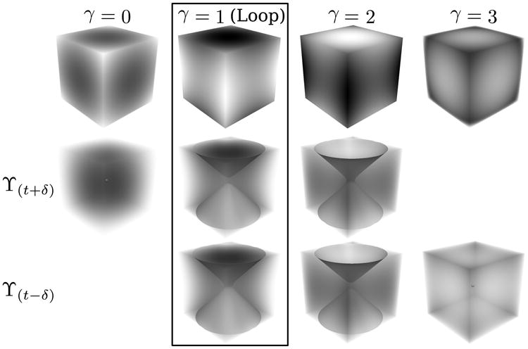
For a Morse function f, all possible critical points, p, are shown on the first row with their indices on top. Upper (ϒ_(t+δ)) and lower (ϒ_(t–δ)) level sets are shown on the second and third rows (for t = f(p) and δ being a small positive number). The case where a loop forms by tracks in TDI is shown in the box.

Localization of loops

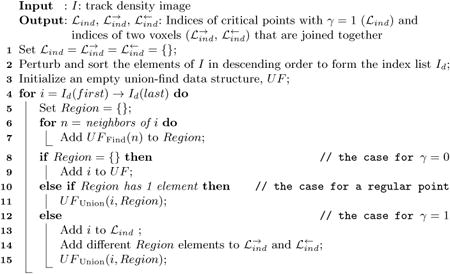
The indices of critical points outline the topology of a scalar field. γ = 0 and γ = 3 are local minima and maxima where level sets vanish and appear. These points correspond to least dense and densest points in TDI. γ=1 and γ = 2 are saddles where level sets split and merge. In a TDI, these points correspond to loops generated by tracks (γ = 1) and empty space (γ = 2), thus our focus are the critical points with γ=1. Fig. 2 shows this case in a box. To find all the critical points, two sweeps are needed, one from top to bottom and another from bottom to top. However, because we are only interested in the critical points with γ = 1, a single sweep from top to bottom is sufficient. Algorithm 1 shows how to identify critical points for detecting loops.

Algorithm 1: Identification of critical points for loop detection

Computation of loop lengths and scoring

We continue by computing loop lengths. In order to do this, we reconstruct a surface mesh for the upper level set (Fig. 2 for γ = 1 and ϒ_(t+δ)). Knowing the two end points of the loop, ${\mathcal{L}}_{\mathit{\text{ind}}}^{\to }$, ${\mathcal{L}}_{\mathit{\text{ind}}}^{\leftarrow }$ from Algorithm 1, we compute the geodesic distance, thus the length of the loop which is used for scoring.

Reeb graphs

To obtain the points on the loop, we compute the Reeb graph of the lower level set (Fig. 2 for γ = 1 and ϒ_(t–δ)). A Reeb graph is an intuitive graph representation of the topological properties of a manifold, M [19]. For a Morse function f: M → ℝ, the Reeb graph, is defined as the quotient space with its topology defined through the equivalent relation x ≃ y if f(x) = f(y) for ∀_{x, y} ∈ M. Here we used the Laplace-Beltrami (LB) eigenfunctions as the Morse function, f. We used the algorithms proposed in [20] for accurate reconstruction the surfaces, computation of LB and the Reeb graph.

3 Test subjects and data preparation

We used the multi-shell HARDI data provided by the human connectome project (HCP) between Q1-Q3 [21] to test our method. This release includes 225 subjects, however, only 215 subjects completed both T1 and dMRI scans. We used these 215 subjects' dMRI data for fiber bundle reconstruction. In order to fully utilize the multi-shell HARDI data and obtain very sharp fiber orientation distributions (FODs), we used the recently proposed algorithm in [22]. This method represents FODs by spherical harmonics (SPHARM) and is fully compatible with existing tools developed for tractography.

We focused on the reconstruction of clean fiber bundles that represent the optic radiation in human brains. To obtain the tracks, we used the probabilistic tractography tool in MRTrix [18] between two automatically generated ROIs: lateral geniculate nucleus (LGN) and primary visual cortex (V1) [23]. One salient feature of the optic radiation is that its fibers are organized retinotopically as they travel from the LGN to the visual cortex. The optic radiation is often considered as composed of three sub-bundles: superior, central, and inferior bundles that correspond to the inferior, foveal, and superior part of the visual field. Most notably the Meyer's loop of the inferior bundle first courses anteriorly before it runs posteriorly toward the visual cortex. This unconventional trajectory is especially challenging for tracking algorithms. To capture the Meyer's loop, it is necessary to lower the curvature threshold in tractography, but this also increases the chance of getting outliers in the result. Thus it is critical to filter out these outliers without sacrificing the ability of capturing the Meyer's loop.

4 Results and discussions

Demonstrative study

Fig. 3 shows an example to demonstrate how our method works. We used fiber bundles from the optical radiation, to be precise, bundles from LGN to V1. We chose these fiber bundles because of their inherent challenge due to Meyer's loop. Because our method is based on removing loops, we aimed to show that our approach is stable, not very sensitive to changes in input parameters and can easily be tuned to preserve important features while removing others. Starting with input tracks, the process in the box (Fig. 3) is iterated until no more removal is possible. The final output is clear of loops that are larger than the threshold provided by the user (14mm in this case). The input tracks shown on the left and the final output on the right are a part of the actual study. The upper (ϒ_(t+δ)) and lower (ϒ_(t-δ)) level sets shown in Fig. 2 are also indicated on top of corresponding surfaces for clarity in Fig. 3.

Fig. 3.

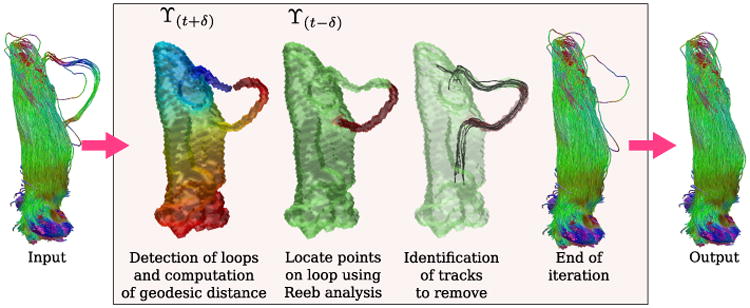
Demonstrative example. Given input tracks, an iterative process shown in the box is run until no more tracks can be removed.

Comparative study against spectral filtering

We compared the results of our method against spectral filtering. For that, we used a similar algorithm to [10]. Fig. 4 shows two different subjects used in our study. Red arrows indicate tracks that should have been removed, green circles indicate tracks that are correctly preserved, i.e: those which project to the primary visual cortex. For our method, we used threshold levels of 12mm and 14mm for the subjects on the left and right respectively. Compared to spectral filtering, our method successfully detects and removes outliers while keeping relevant tracks. Although spectral filtering can be fine tuned for a single subject, this process is complicated, time consuming and not practical for studying populations. On the other hand, our method can easily be tuned with a single geometrically intuitive parameter.

Fig. 4.

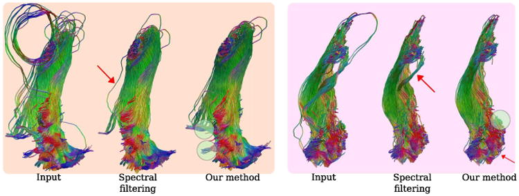
Visual comparison of our method against spectral filtering on two subjects shown in different boxes. Our method keeps some important tracks shown in green circles. Red arrows indicate tracks that should have been removed.

Population study

We applied our method to all the 215 subjects from HCP to obtain a clean reconstruction of the optic radiation using a threshold value of 14mm. According to the post-mortem study in [24], there is a left-ward asymmetry of the optic radiation in human brains. To test this asymmetry in our in-vivo reconstructions, we converted each reconstructed optic radiation into a TDI with 1mm isotropic resolution and counted the number of non-zero voxels as its volume. A two-tailed t-test was then applied to test for differences between left and right hemispheres. Table 1 shows the volumes and the p-value.

Table 1.

Asymmetry of the optic radiation.

	Left hemisphere	Right hemisphere	P-value
Vol (mm3)	1.36E4 ± 2.29E3	1.27E4 ± 1.98E3	9.1E − 11

Earlier research as outlined in section 1 mainly focused on using tractography and anatomical information for categorizing tracks. In contrast, we make use of the track density information with tractography. Therefore we take advantage of the familiar image domain which not only enables us to develop mathematically sound and clear methods but also technically unambiguous and easy to use tools.

To validate the accuracy of our track filtering method, we made a large scale study using 215 subjects from HCP. The results in Table 1 show that, our method produced tracks that show highly significant differences between left and right which is consistent with earlier post-mortem studies [24].

Our current code is in MATLAB^® and C++. Using an Intel^® Core™i7-4700MQ (2.40GHz×8), each block of our method (Fig. 1) is computed in a few seconds. The complete filtering of a single subject takes however ∼5min which is similar to the speed of spectral filtering.

5 Conclusion

We developed a novel technique for filtering out unwanted tracks from tractography. The main contribution of this work is the use of topological analysis for the processing of tracks. Our method provides a geometrically intuitive way of controlling the filtering of outliers. In our experiments, we demonstrated its ability in obtaining cleaner tracks than spectral filtering. We also performed a population study on HCP data and obtained statistically significant results on the left-ward asymmetry of the optic radiation.

References

- 1.Thomas C, Ye FQ, Irfanoglu MO, Modi P, Saleem KS, Leopold DA, Pierpaoli C. Anatomical accuracy of brain connections derived from diffusion MRI tractography is inherently limited. PNAS. 2014;111(46):16574–16579. doi: 10.1073/pnas.1405672111. [DOI] [PMC free article] [PubMed] [Google Scholar]
- 2.Besseling R, Jansen J, Overvliet G, Vaessen M, Braakman H, Hofman P, Aldenkamp A, Backes W. Tract specific reproducibility of tractography based morphology and diffusion metrics. PLoS ONE. 2012;7(4) doi: 10.1371/journal.pone.0034125. [DOI] [PMC free article] [PubMed] [Google Scholar]
- 3.Girard G, Whittingstall K, Deriche R, Descoteaux M. Towards quantitative connectivity analysis: reducing tractography biases. NeuroImage. 2014;98:266–278. doi: 10.1016/j.neuroimage.2014.04.074. [DOI] [PubMed] [Google Scholar]
- 4.Fillard P, Descoteaux M, Goh A, Gouttard S, Jeurissen B, Malcolm J, Ramirez-Manzanares A, Reisert M, Sakaie K, Tensaouti F, Yo T, Mangin JF, Poupon C. Quantitative evaluation of 10 tractography algorithms on a realistic diffusion MR phantom. NeuroImage. 2011;56(1):220–234. doi: 10.1016/j.neuroimage.2011.01.032. [DOI] [PubMed] [Google Scholar]
- 5.Mangin JF, Fillard P, Cointepas Y, Le Bihan D, Frouin V, Poupon C. Toward global tractography. NeuroImage. 2013;80:290–296. doi: 10.1016/j.neuroimage.2013.04.009. [DOI] [PubMed] [Google Scholar]
- 6.Daducci A, Dal Palu A, Lemkaddem A, Thiran JP. COMMIT: Convex Optimization Modeling for Microstructure Informed Tractography. IEEE Transactions on Medical Imaging. 2015 Jan;34(1):246–257. doi: 10.1109/TMI.2014.2352414. [DOI] [PubMed] [Google Scholar]
- 7.Pestilli F, Yeatman J, Rokem A, Kay K, Wandell B. Evaluation and statistical inference for living connectomes. Nature methods. 2014 Oct;11(10):1058–1063. doi: 10.1038/nmeth.3098. [DOI] [PMC free article] [PubMed] [Google Scholar]
- 8.Smith RE, Tournier JD, Calamante F, Connelly A. SIFT: Spherical-deconvolution informed filtering of tractograms. NeuroImage. 2013 Feb;67:298–312. doi: 10.1016/j.neuroimage.2012.11.049. [DOI] [PubMed] [Google Scholar]
- 9.Xia Y, Turken A, Whitfield-Gabrieli S, Gabrieli J. Knowledge-based classification of neuronal fibers in entire brain. In: Duncan J, Gerig G, editors. MICCAI 2005. Springer Berlin; Heidelberg: 2005. pp. 205–212. Volume 3749 of LNCS. [DOI] [PubMed] [Google Scholar]
- 10.O'Donnell L, Westin CF. Automatic Tractography Segmentation Using a High-Dimensional White Matter Atlas. IEEE Trans Med Img. 2007;26(11):1562–1575. doi: 10.1109/TMI.2007.906785. [DOI] [PubMed] [Google Scholar]
- 11.Brun A, Knutsson H, Park HJ, Shenton M, Westin CF. Clustering fiber traces using normalized cuts. In: Barillot C, Haynor D, Hellier P, editors. MICCAI 2004. Springer Berlin; Heidelberg: 2004. pp. 368–375. Volume 3216 of LNCS. [DOI] [PMC free article] [PubMed] [Google Scholar]
- 12.Tsai A, Westin CF, Hero A, Willsky A. Fiber Tract Clustering on Manifolds With Dual Rooted-Graphs. Proc CVPR. 2007:1–6. [Google Scholar]
- 13.Wassermann D, Bloy L, Kanterakis E, Verma R, Deriche R. Unsupervised white matter fiber clustering and tract probability map generation: Applications of a Gaussian process framework for white matter fibers. NeuroImage. 2010;51(1):228–241. doi: 10.1016/j.neuroimage.2010.01.004. [DOI] [PMC free article] [PubMed] [Google Scholar]
- 14.Li H, Xue Z, Guo L, Liu T, Hunter J, Wong STC. A hybrid approach to automatic clustering of white matter fibers. NeuroImage. 2010;49(2):1249–1258. doi: 10.1016/j.neuroimage.2009.08.017. [DOI] [PubMed] [Google Scholar]
- 15.Wang X, Grimson WEL, Westin CF. Tractography segmentation using a hierarchical Dirichlet processes mixture model. NeuroImage. 2011;54(1):290–302. doi: 10.1016/j.neuroimage.2010.07.050. [DOI] [PMC free article] [PubMed] [Google Scholar]
- 16.Calamante F, Tournier JD, Jackson GD, Connelly A. Track-density imaging (TDI): Super-resolution white matter imaging using whole-brain track-density mapping. NeuroImage. 2010;53(4):1233–1243. doi: 10.1016/j.neuroimage.2010.07.024. [DOI] [PubMed] [Google Scholar]
- 17.Calamante F, Tournier JD, Kurniawan ND, Yang Z, Gyengesi E, Galloway GJ, Reutens DC, Connelly A. Super-resolution track-density imaging studies of mouse brain: Comparison to histology. NeuroImage. 2012;59(1):286–296. doi: 10.1016/j.neuroimage.2011.07.014. [DOI] [PubMed] [Google Scholar]
- 18.Tournier JD, Calamante F, Connelly A. MRtrix: Diffusion tractography in crossing fiber regions. Int J of Imag Syst Tech. 2012;22(1):53–66. [Google Scholar]
- 19.Edelsbrunner H, Harer J. Computational Topology: An Introduction. American Mathematical Soc. 2010 [Google Scholar]
- 20.Shi Y, Lai R, Toga AW. Alzheimers Disease Neuroimaging Initiative: Cortical surface reconstruction via unified Reeb analysis of geometric and topological outliers in magnetic resonance images. IEEE Trans Med Img. 2013;32(3):511–530. doi: 10.1109/TMI.2012.2224879. [DOI] [PMC free article] [PubMed] [Google Scholar]
- 21.Essen DV, Ugurbil K, Auerbach E, Barch D, Behrens T, Bucholz R, Chang A, Chen L, Corbetta M, Curtiss S, Penna SD, Feinberg D, Glasser M, Harel N, Heath A, Larson-Prior L, Marcus D, Michalareas G, Moeller S, Oostenveld R, Petersen S, Prior F, Schlaggar B, Smith S, Snyder A, Xu J, Yacoub E. The human connectome project: A data acquisition perspective. NeuroImage. 2012;62(4):2222–2231. doi: 10.1016/j.neuroimage.2012.02.018. [DOI] [PMC free article] [PubMed] [Google Scholar]
- 22.Tran G, Shi Y. Fiber Orientation and Compartment Parameter Estimation from Multi-Shell Diffusion Imaging. IEEE Transactions on Medical Imaging. 2015 doi: 10.1109/TMI.2015.2430850. in press. [DOI] [PMC free article] [PubMed] [Google Scholar]
- 23.Benson NC, Butt OH, Datta R, Radoeva PD, Brainard DH, Aguirre GK. The retinotopic organization of striate cortex is well predicted by surface topology. Current Biology. 2012;22(21):2081–2085. doi: 10.1016/j.cub.2012.09.014. [DOI] [PMC free article] [PubMed] [Google Scholar]
- 24.Burgel U, Schormann T, Schleicher A, Zilles K. Mapping of histologically identified long fiber tracts in human cerebral hemispheres to the MRI volume of a reference brain: Position and spatial variability of the optic radiation. NeuroImage. 1999;10(5):489–499. doi: 10.1006/nimg.1999.0497. [DOI] [PubMed] [Google Scholar]