Heterogeneous views on heterogeneity

The insightful and stimulating commentary by Julian Higgins¹ on our paper² raises several important issues that need to be clarified. First, we need to agree on nomenclature. The heterogeneity literature has been plagued by inconsistent terminology. Terms like ‘heterogeneity’, ‘inconsistency’, ‘variation’, ‘diversity’, ‘between-study variance’, ‘variability’, etc. are used interchangeably. While Higgins prefers the term ‘inconsistency’ for I², in other writings he has used the words ‘variability’ and ‘heterogeneity’ in association with this measure.³ We believe that the term ‘heterogeneity’ is a nice word with roots going back to ETEPOΓENHΣ of Aristotle and ETEPOΓENΩΣ of Sextus Empiricus. It can be applied to any of the popular metrics and tests, but then one simply has to specify which metric or test is exactly alluded to. ‘Inconsistency’ is also a nice, more recent word, but again we need to clarify what it refers to each time.

Higgins worries about ‘the post hoc hypotheses that need to be thought up to explain why the excluded studies might be outlying or influential’. We were clear cut in our paper that this is indeed not an easy task. We believe that sensitivity analyses, as currently performed, are usually an invitation to post hoc data dredging with few or no rules in the game. This reduces their inferential reliability. However, this is a major reason why our proposed algorithms may offer one way to improve this free-lunch situation. There are two components to any sensitivity analysis. The first component is how it is done. The second component is how the results are interpreted. We argue that our method takes away much of the subjectivity in the first component. We do not wish to diminish the uncertainty that arises in the second component, and we wish that all meta-analysts recognize and acknowledge this uncertainty properly.

Higgins questions whether it is sensible to define a ‘desired’ threshold in terms of I² statistic. Although we agree that indeed ‘(some) heterogeneity is to be expected in (almost any) meta-analysis’ and ‘any amount of heterogeneity is acceptable, providing both that the predefined eligibility criteria for the meta-analysis are sound and that the data are correct’, we believe that using thresholds to describe heterogeneity is an unavoidable consequence of the effort to translate statistical terms into real life. Higgins and colleagues have faced this problem, similarly recommending categorization of values for I² and assigning adjectives of low, moderate, and high heterogeneity or inconsistency.^4,5 In our article we have used these values of 50% and 25% for I², as traditional thresholds for large and moderate heterogeneity, respectively. This does not negate the need to recognize the major uncertainty in heterogeneity estimates,⁶ but provides a standardized approach that can be applied consistently across meta-analyses.

Higgins argues in favour of using τ², the estimate of between-study variance, rather than I² in our paper, because I² depends also on the within-study precisions. Actually I² has become popular as a measure primarily due to the groundbreaking work of Higgins.^3,4 I² is one of the most commonly reported heterogeneity (or inconsistency) metrics, while the between-study variance τ² is rarely reported in the medical literature. I² has an intuitive interpretation, and it is comparable across meta-analyses with different numbers of studies or different types of effect metrics, whereas τ² is difficult both to understand and compare, according to Higgins’ writings.² Therefore, we focused on I² in our paper. However, the algorithms that we have proposed are not applicable only to I². These are general methods that can be used with any kind of metric, e.g. τ². If another metric may be useful to apply more widely, we would rather suggest h, the ratio of τ over the absolute value of the normalized summary effect (e.g. log odds ratio).⁷ This h is not to be confused with yet another heterogeneity metric, H capital, which is the square root of the chi-squared heterogeneity statistic divided by its degrees of freedom.² The major problem with τ² for an epidemiologist is that it means almost nothing when seen in isolation. The same τ² value could be huge or negligible depending on what the summary effect is, and what impact that between-study variance has in shaping the upper and lower bounds of the summary effect confidence interval. We are in the process of implementing the sensitivity analysis algorithm on other heterogeneity metrics and we will release the new software module when it is properly beta-tested.

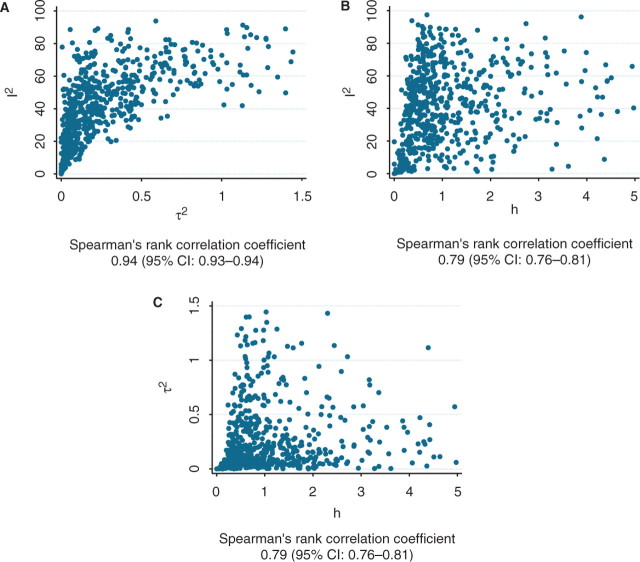
Regardless, at a practical level, τ² and I² tend to be largely concordant, when examined across many meta-analyses. In Figure 1 we illustrate the correlation between I² and τ² in the Cochrane meta-analyses database (n = 1011 meta-analyses) used in our article: the rank correlation coefficient is as high as 0.93. For comparison, the correlation coefficients for h against τ² and for h against I² are both 0.79 (Figure 1).

Figure 1.

Correlation between (A) I² and τ² (B) h and τ² and (C) h and I² in the meta-analyses of the Cochrane database

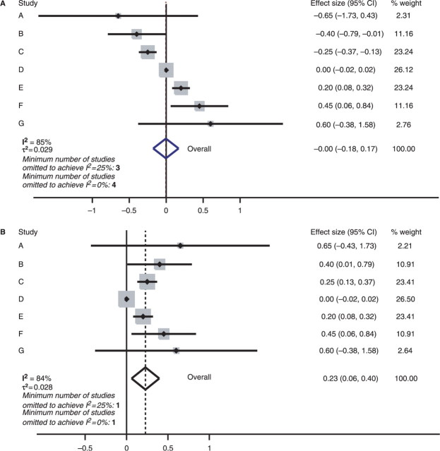
Higgins uses also a simulated example to illustrate why I² is not a sensible metric. He notes that I² behaves differently than τ² when there are different within-study errors among the studies. This is expected since these two metrics, although highly correlated, are not interchangeable. Specifically, the sequential algorithm is used to demonstrate that the drop in I² is not correlated with the drop in τ², rather τ² increased in the intermediate steps till the goal (I² = 0%) is achieved. However, in that same example, using the combinatorial algorithm one can find a combination of four studies (D, E, F, G) whose exclusion results in an I² value of 0% (95% CI 0–73%) and also τ² of 0. The fact that the two algorithms give such different results reflects the complex and persistent inconsistency of this peculiar simulated meta-analysis. This is visible even in the forest plot. We argue that I² and τ² alone do not suffice to describe this complexity, and our sensitivity algorithms offer additional information.

To illustrate this, let us compare the meta-analysis simulated by Higgins (Figure 2A) vs another meta-analysis where, starting from the same data, all the individual effect sizes are coined to be ≥0 (Figure 2B). The new simulated meta-analysis has an I² value of 84% (95% CI 65–90%) and τ² of 0.028, values almost identical to the ones in Higgins’ example. The gross differences between these two meta-analyses can be seen even inspecting their forest plots, but both I² and τ² have very similar values. Applying the sequential algorithm to our simulated example, I² becomes 0% (95% CI 0–75%) and τ² becomes 0 with omission of a single study (study D). This example illustrates that meta-analyses with the same I² and τ² may require a very different number of studies to be omitted to decrease I² to a certain level or 0%. The underlying heterogeneity cannot be described or quantified by a single metric. We therefore recommend that routinely it may be worthwhile reporting this information besides just I² and/or τ² or any other heterogeneity metric.

Figure 2.

Simulated meta-analyses. (A) is the same as the second example of Higgins, while (B) is a simulated example where all effect sizes have been coined to be ≥0, while otherwise the data are identical to (A). Note that even though the two meta-analyses have very similar I² and τ², they require a different number of studies to be omitted to diminish heterogeneity

References

- 1.Higgins JP. Heterogeneity in meta-analyses should be expected and appropriately quantified. Int J Epidemiol. 2008;37:1158–60. doi: 10.1093/ije/dyn204. [DOI] [PubMed] [Google Scholar]
- 2.Patsopoulos NA, Evangelou E, Ioannidis JPA. Sensitivity of between-study heterogeneity in meta-analysis: proposed metrics and empirical evaluation. Int J Epidemiol. 2008;37:1148–57. doi: 10.1093/ije/dyn065. [DOI] [PMC free article] [PubMed] [Google Scholar]
- 3.Higgins JPT, Thompson SG. Quantifying heterogeneity in a meta-analysis. Stat Med. 2002;21:1539–58. doi: 10.1002/sim.1186. [DOI] [PubMed] [Google Scholar]
- 4.Higgins JPT, Thompson SG, Deeks JJ, Altman DG. Measuring inconsistency in meta-analyses. Br Med J. 2003;327:557–60. doi: 10.1136/bmj.327.7414.557. [DOI] [PMC free article] [PubMed] [Google Scholar]
- 5.Higgins J, Green S, editors. Cochrane Handbook for Systematic Reviews of Interventions Version 5.0.0 [updated February 2008]. The Cochrane Collaboration. 2008 [Google Scholar]
- 6.Ioannidis JP, Patsopoulos NA, Evangelou E. Uncertainty in heterogeneity estimates in meta-analyses. Br Med J. 2007;335:914–16. doi: 10.1136/bmj.39343.408449.80. [DOI] [PMC free article] [PubMed] [Google Scholar]
- 7.Moonesinghe R, Khoury MJ, Liu T, Ioannidis JP. Required sample size and nonreplicability thresholds for heterogeneous genetic associations. Proc Natl Acad Sci USA. 2008;105:617–22. doi: 10.1073/pnas.0705554105. [DOI] [PMC free article] [PubMed] [Google Scholar]