Abstract
In recent years, there has been considerable interest in visual attention models (saliency map of visual attention). These models can be used to predict eye fixation locations, and thus will have many applications in various fields which leads to obtain better performance in machine vision systems. Most of these models need to be improved because they are based on bottom-up computation that does not consider top-down image semantic contents and often does not match actual eye fixation locations. In this study, we recorded the eye movements (i.e., fixations) of fourteen individuals who viewed images which consist natural (e.g., landscape, animal) and man-made (e.g., building, vehicles) scenes. We extracted the fixation locations of eye movements in two image categories. After extraction of the fixation areas (a patch around each fixation location), characteristics of these areas were evaluated as compared to non-fixation areas. The extracted features in each patch included the orientation and spatial frequency. After feature extraction phase, different statistical classifiers were trained for prediction of eye fixation locations by these features. This study connects eye-tracking results to automatic prediction of saliency regions of the images. The results showed that it is possible to predict the eye fixation locations by using of the image patches around subjects’ fixation points.
Keywords: Visual attention model, Saliency map, Eye fixation, Bottom-up and top-down attention, Semantic content, Eye tracking
Introduction
Recently, there has been much interest in the visual attention models that they can be applied for prediction of eye fixation locations. These models show a saliency map for each visual image for the fixation points. The more salient locations in the map present locations with high probability of being eye fixation points (Fig. 1). Developing models that automatically predict the eye fixations, imitate the human visual mechanism. So using these models as a part of machine vision systems have many advantages and applications (Zhang and Lin 2013). These models can be used to obtain better performance in terms of increasing the speed and reducing the data storage in machine vision systems (Rajashekar et al. 2003). Some of the applications of visual attention models includes automatic object recognition and detection, automatic guidance of vehicles, image compression, better performance in human computer interaction, face recognition and particularly fast selection of the regions of interest (ROI) in complex visual scenes (Geisler and Perry 1998; Wang et al. 2003; Viola and Jones 2001; DeCarlo and Santella 2002; Jaimes et al. 2001; Wang et al. 2013; Itti and Koch 2001).
Fig. 1.
a The original image (used in our experiment). b Eye fixation points of fourteen individuals while viewing the typical image. c Actual saliency map result of eye fixation points (the saliency map created by convolving a Gaussian filter over the eye fixation locations of all individuals)
It is possible to recognize objects on different part of the scene by focusing attention each time on different locations. Actually, we are not able to perceive everything around us. The results of experiments indicate that a detailed representation of our environments is not formed in our brain and attention is a mechanism to perceive the changes (Rensink et al. 1997). The visual attention directs the processing of the brain to focus on important regions of visual field and to search a target in complex scenes (Posner 1980). The two types of visual attention are namely overt visual attention, which includes eye movements, and covert visual attention, which does not need eye movements (Henderson et al. 2007). In this study, by “visual attention” we refer to the overt visual attention. Previous studies (Yarbus 1967) have shown that attention depends on both bottom-up information and top-down signals which they maybe show two mechanisms of visual attention in the brain. These two mechanisms are called bottom-up attention (exogenous) and top-down attention (endogenous). Bottom-up attention is fast, involuntary and task-independent while top-down attention is slow, voluntary, task-dependent. Due to importance of visual attention mechanism in visual information processing, modeling of attention has been the focus of many studies in recent years (Filipe and Alexandre 2013). The “Feature Integration Theory” of Treisman & Gelade has been the basis of many theoretical models in the past (Borji and Itti 2013). One of the early models of visual attention was proposed by Koch and Ullman (1985). They proposed a feed-forward model to combine low-level features to create a saliency map that represents conspicuousness of scene locations. A winner-take-all neural network in their model selects the most salient locations. A mechanism of inhibition of return then permits the focus of attention to shift to the next most salient location. Other models have been proposed based on this idea that could process digital images (Borji and Itti 2013). Itti et al. (1998) proposed the first approach for implementation of the Koch & Ullman model. Many more implementations of visual attention model have been presented then after. For example, Yu et al. proposed a computational model of visual attention based on a pulsed principal component analysis (PCA) transform. This model considers the signs of the PCA coefficients for creating spatial and motional saliency. This idea was extended to a pulsed cosine transform too, which was data-independent and very fast (Yu et al. 2011). Bian and Zhang (2010) proposed a biologically plausible model for visual saliency detection, which is called frequency domain divisive normalization. The proposed method is a fast frequency domain saliency detection approach. In Gu and Liljenström (2007) a neural network model for attention has been proposed. The structure of this model consists of a multi-scale network and is involved in many higher level information processing tasks (Gu and Liljenström 2007). There are two different views to computational models of bottom-up visual attention (Le Meur 2014). One group assumes that there is a unique saliency map (Koch and Ullman 1985; Li 2002). The other group thinks that there are several saliency maps spread throughout the visual areas. Different brain areas (such as LIP and MT cortex) are considered to be the candidate for computation of the saliency map (Le Meur 2014; Lanyon and Denham 2009).
The debate between these two groups become more complicated as the term of the “saliency” is used differently in the literature. Some use it for bottom-up aspects of prioritization and some others use salience and priority interchangeably [see Borji and Itti (2013), Awh et al. (2012) for more information].
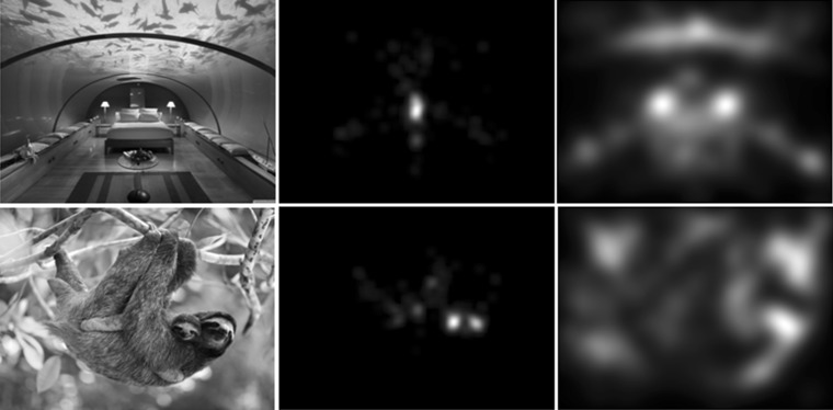
The visual attention models can be grouped into three general categories namely biologically inspired models, probabilistic models and machine learning models (Borji and Itti 2013; Le Meur 2014). Of course, a model can be considered as a mixture of two or three classes mentioned above (Zhang et al. 2008). In biologically inspired models, the image features at different scales are grouped into a saliency map and then a neural network scans the attended locations based on the decreasing order of the saliency in the map (Itti et al. 1998; Le Meur et al. 2006; Marat et al. 2009). The probabilistic models use a probabilistic framework based on the information theory in their structure. Based on the studies in the human visual system, these models consider the contextual information of the scene for finding the informative regions of the images. The first model in this category has been proposed by Oliva et al. (2003; Zhang et al. 2008). Machine learning-based approaches combine different low-level, mid-level and high-level features for training a classifier. For example, in Judd et al. (2009) different low-level features like the local energy of the steerable pyramid sub-bands filters in different orientations and different scales, the values of the red, green and blue channels and some other features were used beside the support vector machine classifier to train the model. In Shen and Zhao (2014) a model based on the hierarchical structure of feature extraction in the ventral stream in the visual cortex is proposed. The model predicts the saliency by learning from the natural images and at multiple stages of features. The features are integrated and the weights of this integration are computed based on the ground-truth fixation data. Although most of the proposed models qualitatively work well, their use is limited because their outputs do not meet well with actual human fixations data (Judd et al. 2009). Most of these models do not consider the top-down semantic information and they use just the bottom-up features in their structure, so they need to be improved to be able to match actual eye fixation locations (Awh et al. 2012; as depicted in Fig. 2). There is also an important distinction between top-down in the sense of “task-driven” and higher-level content. By top-down models, we mean those models that consider higher-level content. The Fig. 2 shows two samples of the images used in our experiment, which compare real saliency map (which is from eye movement data of participants in our experiment) and the saliency map of Itti and Koch model.
Fig. 2.
Left column original images shown to the subjects, middle column the resulting actual saliency map of the subject’s eye-tracking data and right column Itti and Koch saliency map for two sample images. As can be seen, current attention models do not accurately predict people’s eye fixation locations
In this study, we recorded the eye movements of fourteen individuals while viewing the gray scale images of two different semantic categories. We extracted the fixation locations of eye movements in two image categories as patches of images around the eye fixation points. After extraction of the fixation areas, characteristics of these areas were evaluated and were compared to non-fixation areas.
The extracted features include the orientation and spatial frequency. After feature extraction phase, different statistical classifiers were trained for predicting the eye fixation locations in new images. Indeed, we explored the way in which individuals look at images of different semantic categories, and related those results to approaches for automatic prediction of eye fixation locations. Our study connects eye-tracking results to automatic prediction of saliency regions of the images. The results show that it is possible to predict the eye fixation locations by using of the image patches around subjects’ fixation points. In addition, the efficacy of the low-level visual features in attracting the eye movements is affected by the high-level image semantic information.
The rest of the paper has been organized as follows: “Procedure and methods” section presents the procedure and methods of the experiment (participants, stimuli, procedure and paradigm) and describes the approach we have applied to track the subjects’ eye movements. In “Controlling low-level features of the image” section, we compare the low-level features in the images of two different semantic categories that shown to the subjects. In “Definition and extraction of eye fixations data” section, eye fixations data is defined and extracted. “Predicting eye fixation locations” section is dedicated to methods (creating feature vectors, training different classifiers,…) and results related to prediction of the eye fixation locations and creating the saliency map (attention model). In “Performance and evaluation” section, we evaluate the performance of the model on our data set and Toronto data set. “The discussion and conclusions” section presents the relevant discussion and conclusions.
Procedure and methods
Participants
Fourteen subjects (four females and ten males, aged between 22 and 30 years; standard deviation of 2.03 years) participated in our experiment. The participants had normal or corrected-to-normal visual acuity and had no history of eye and muscular diseases. The participants were the students and researchers at the school of Cognitive Science, Institute for Research in Fundamental Sciences (IPM-Tehran, Iran). All participants were naive to the purposes of the experiment. Informed consent was obtained for experimentation from the subjects. The work was carried out in accordance with the Code of Ethics of the World Medical Association (Declaration of Helsinki).
Stimuli
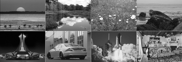
We used 18 gray scale images from each of two semantic different categories (in total 36 images) as stimuli including the natural images (included natural scenes such as landscape, animal) and the man-made images (included man-made scenes such as building, vehicles). Each image had a size of 700 × 550 in pixels. A small size of several images has been shown in Fig. 3. There were no artificial object in natural images and no natural object in man-made images.
Fig. 3.
Eight samples of the 36 images used in the experiment (from each of the two categories), top row natural category, bottom row man-made category. They were resized for viewing here
Procedure
In order to record the eye movements of the participants in the experiment, we have used the infrared, video-based eye tracker system of EyeLink1000 (SR Research, Canada). We set the sampling rate of eye tracker device in 1000 Hz in the monocular (left eye) Pupil-CR recording mode. The experiments were done in a small dark room that was insulated in terms of light and sound (in order to eliminate the distracters). We controlled the drift and did a new calibration when necessary (while drift was larger than of 0.5° of visual angle). A chinrest was used in order to avoid from participant’s head movements. Participants were seated 57 cm from the screen of the monitor. The Images were displayed on the center of an LG 21-inch flat panel screen with a resolution of 1024 × 768 pixels and refresh rate of 75 Hz. With these conditions, every 20 pixels of the displayed image will be equivalent to 1° of visual angle.
Paradigm
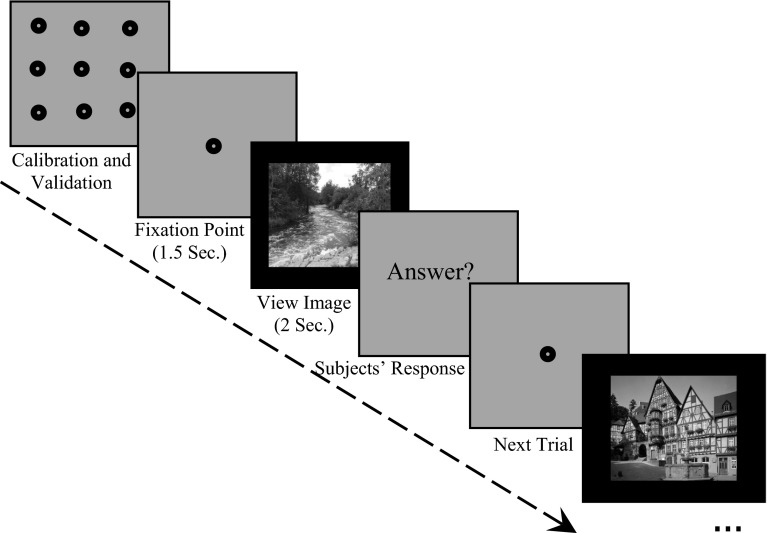
Eye movement data of fourteen subjects were recorded during the experiment as the subjects viewed images from the two categories in three blocks of trials. In each block, 36 images (18 images from natural and 18 images from man-made category) were shown randomly to the subjects (totally, each subject viewed 108 images). At the beginning of each block of the trials, the 9-point calibration and 11-point validation procedures were performed (in order to ensure the lack of subjects’ head movement until the end of each block). In each block after calibration and validation procedures, the subjects were shown a fixation point with a time duration of 1.5 s located in the center of the screen (to ensure that the starting point of the eye movements begins at the center of the screen for all images) and then each image was displayed for 2 s. After this time, a page appeared that asked the answer of the subjects (“Answer”, in order to engage the persons to perform the task). The subjects were instructed to press “left arrow” on the keyboard if the image was belonging to the natural category and “right arrow” on the keyboard if the image was belonging to the man-made category. One second after the answer (in order to eliminate the effect of hand motion on the eye movements) next fixation point was appeared and was followed by the next image. This procedure was continued until the end of the block. The experimental steps are illustrated in Fig. 4. We recorded the subjects’ eye movements during the whole experiment. If the subjects did not focused on the fixation point at the beginning of the trials, their data was removed from the analysis for those trials. All subjects fixated on fixation point at the beginning of the trials and only one subject in two trials in two different blocks, focused on distance away from the fixation point. A radius distance more than six pixels from the fixation point was the criterion for being “not focused”. The first fixation points on eye movements were eliminated from the analysis.
Fig. 4.
Paradigm design. At the beginning of each block of trials a calibration and a validation procedure were performed. After this, a fixation point was appeared for a duration of 1.5 s located in the center of the screen, and then, each image was displayed for 2 s. Then one page was appeared that asked for the answer of the subjects “Answer”. The next fixation point (next trial) was appeared 1 s after the answer and followed by the next image
Controlling low-level features of the image
We use the gray scale images because our purpose is to predict fixation locations in visual scenes with different semantic content, and as we know, the “contents” of image is independent of the “color” of it. For example, we see the image of a forest and we perceive it is a forest, either its color is green or black and white (gray scale).
We intended to investigate the image semantic and conceptual effects on the subjects’ eye movements. Indeed, our purpose was predicting the eye fixation locations in the visual scenes with different semantic contents. Required for this claim is that we control the images’ low-level features in two categories as far as possible and make sure that these features are not significantly different between the two categories of gray scale images. To achieve this, we have investigated the mean of gray scale value, histogram distribution, spatial frequency and edge density parameters in both sets of images. Clearly, there are some other properties that controlling and unification of them is not simply possible. It should be noted that property of “edge density” which is compared between images, could be a criterion of number of objects in each image. The more the objects, the more the intensity of edges in each image (each object is mainly recognized by its edges).
The results of this control indicated that there was no significant difference between two groups regarding the mean of gray scale value (average value for all images ± the standard error of the mean; natural = 97.56 ± 7.83, man-made = 101.43 ± 7.25; T test: p = 0.72 and Wilcoxon rank-sum test: p = 0.76, the degrees of freedom (df) = 2n-2 = 34) and the spatial frequency (natural = 0.22 ± 0.01, man-made = 0.2 ± 0.004; T test: p = 0.11 and Wilcoxon rank-sum test: p = 0.22, df = 34) parameters. (Significance level α = 0.05 and in a two-sided (two-tailed) test condition, for all comparative tests in this paper). The method of obtaining a measure of the images’ spatial frequency has been mentioned in the following subsection.
Spatial frequency
To calculate and obtain a measure of the images’ spatial frequency, first we applied the 2D Discrete Fourier Transform (2D-DFT) on each image. In digital image processing, each image function f(x, y) is defined over discrete instead of continuous domain, finite or periodic.
The transform of an N × N image yields an N × N array of Fourier coefficients that completely represent the original image. After obtaining the complex coefficients F (u, v) (Real, R (u, v), and imaginary, I (u, v) parts; Eq. 1) for each of the images, magnitude of all coefficients (amplitude spectrum, ; Eq. 2) are calculated:
| 1 |
| 2 |
The number of Fourier coefficients that their amplitude is larger than a threshold value was calculated for each of the images separately, as a measure of the spatial frequency of the image. We considered the threshold value equal to the average amplitude of the Fourier coefficients for each image separately. Finally, this measure was normalized to the number of all the Fourier coefficients of each image (equal to the number of all pixels of each image).
Image histogram
For image histogram parameters, due to the fact that most of the images had a similar shape of the histogram distribution (single-mode distribution), we matched all the image histograms with the histogram of one of image. Therefore, all the images (natural and man-made) had almost a similar form of histogram (single-mode distribution). This caused the images have a similar shape of histograms.
Edge density
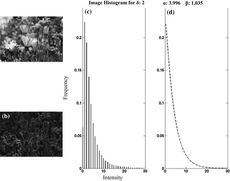
Another important parameter is the edge density of the images used in the experiment. To evaluate this parameter, first, the edges of the image were extracted by applying Gaussian derivative filters, and then, the Weibull probability distribution function (Eq. 3; Geusebroek and Smeulders 2002) was fitted to the histogram of the images contained the information of the extracted edges (Fig. 5). For each image Weibull function parameters (scale parameter (α) and shape parameter (β)) were extracted and the mean values of these parameters were compared between the two groups of images. The results showed that there was no significant difference between groups neither for α parameter (natural = 3.23 ± 0.3, man-made = 3.38 ± 0.31; T test: p = 0.71 and Wilcoxon rank-sum test: p = 0.68, df = 34) nor the β parameter (natural = 0.78 ± 0.05, man-made = 0.77 ± 0.04; T test: p = 0.87 and Wilcoxon rank-sum test: p = 0.97, df = 34).
| 3 |
Fig. 5.
a A sample image shown to the subjects. b The edges that were extracted from the image. c Histogram of the extracted edges and, d Fitting a Weibull function to the resulting histogram
Definition and extraction of eye fixations data
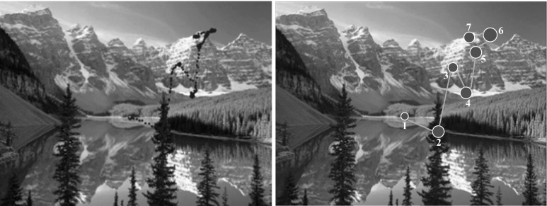
We plotted the subjects’ eye movement data on the corresponding images and we derived the fixations and rapid jumps of the eye movements (saccade) from the data. In this study, our definition of fixation and saccade was respectively as follows: A location was considered as fixation when the eyes remained for at least 80 ms in locations of images whit maximum space of 0.5° of visual angle. Saccades were detected when the eyes were displaced with minimum jump amplitude of 1.5° of visual angle and minimum speed of 22° of visual angle per second. Nevertheless, we used only the fixation points in our analysis and in practice we do not deal with saccades. In Fig. 6 (left), the path of eye movements has been shown by blue dots for one of the subjects. In addition, in Fig. 6 (right), Purple circles represent the eye fixation areas and the cyan lines connecting the circles represent the possible saccades (some of the lines and not all of them by considering the conditions of the amplitude and speed to eye movements). Temporal order of the fixation points have been marked on image with the numbers from 1 to 8. After extracting the subjects’ eye fixations points, the relevant image patches were also extracted that we explain them in the rest of paper.
Fig. 6.
Left the subjects’ pattern of eye movements while viewing an image (blue dots), right the fixation locations of the eye (purple circles) and saccades (some of the cyan lines). (Color figure online)
Predicting eye fixation locations
The aim of our research is to predict the eye fixation locations in two image categories and ultimately, to create a saliency map for each image (attention model). First step of the analysis is allocated to the feature extraction phase. In this step, we extract the actual subjects’ eye fixation points and then the features from these points are extracted. We control whether these features are different from the features of the control points (random points) significantly. After feature extraction step, we use the different classifiers in order to classify the eye fixation and non-fixation locations in the images. Indeed, we propose to learn a visual attention saliency model directly from the human eye movement data.
Method and analysis
In the first part of the analysis, the goal is to extract the features of the eye fixation locations that are different between the fixation and non-fixation locations (control locations) significantly. To this end, image patches with different sizes from two different image categories were extracted around the eye fixation points and around the control points. For each image control patches (control locations) were selected quite randomly, so that these patches had no overlap or subscription with patches around the fixation points (The extracted patches around the fixation points had not any overlap with those around the control points). Each of the patches is used to form a feature vector for each of the locations.
Modeling the simple and complex cells in the primary visual cortex
The neurobiological studies on the neural mechanism of vision showed that a multi-level network with a feedback control can achieve orientation detection instantaneously and the results are finally stored in the primary visual cortex (Wei et al. 2013). Here we give a brief description of modeling the simple and complex cells in the primary visual cortex which has been used as a part of feature extraction.
The first cells in the cortex that analyze the visual information are simple cells in the primary visual cortex (Serre and Riesenhuber 2004). Gabor filters provide a good model for cortical simple cell receptive fields (Serre and Riesenhuber 2004; Serre et al. 2005; Riesenhuber and Poggio 2000). The following equations describe the cortical simple cell receptive field models mathematically:
| 4 |
| 5 |
| 6 |
The five Gabor filter parameters, i.e., effective width σ, aspect ratio Y = 0.3, orientation θ, wavelength λ and filter sizes s (RF size) were adjusted so that the tuning properties of the corresponding simple units match the V1 para foveal simple cells based on the data from two groups: De Valois et al. (1982a, b) and Schiller et al. (1976a, b, c). In this study, we arranged the simple filters in two filter sizes of 11 × 11 and 13 × 13 pixels (Band 2). Although we tried other bands (Band 1 containing two filter sizes of 7 × 7 and 9 × 9 pixels and Band 3 containing two filter sizes of 15 × 15 and 17 × 17 pixels) there was no significant difference in the performance of our model, so we used the filters only from Band 2. In addition, we considered four orientations (0°, 45°, 90° and 135°), thus leading to eight different simple receptive field types in total (2 scales × 4 orientations) for each of the patches extracted from the images (the fixation and control patches). This is a simplification in the model but this has been shown to be adequate to provide rotation and size invariance in good agreement with recordings in infero-temporal cortex (IT) (Riesenhuber and Poggio 1999).
The next step in the processing of visual information in the cortex is performed by the cortical complex cells. These cells are to some extent invariant to shift (position) and size. They have larger receptive field as compared to simple cells (Serre and Riesenhuber 2004). Complex cells receive inputs from simple cells in the previous layer with the same orientation and scale properties. The scale band index of the simple units also determines the size of the simple neighborhood N × N over which the complex units pool (Eq. 7). This procedure was done for each of the four orientations independently.
| 7 |
The corresponding pooling operation is a MAX operation, which increases the tolerance to -D transformations from layer simple to complex. So, the response of a complex cell is obtained through the maximum response of its N × N afferents from the previous simple layer such that:
| 8 |
For each orientation, there are two simple maps (in every one of the bands that we used from band 2): The one obtained using a filter of size 11 × 11 and the one obtained using a filter of size 13 × 13. The complex cell responses are calculated by subsampling these maps using a cell grid of size 10 × 10 (N = 10). A maximum value is then taken from 100 elements in the grid. The max operation is finally used over the two scales. The complex units overlapped by an amount of five pixels (N/2). The parameters were fixed according to the experimental data [see Serre et al. (2005) for details].
Creating feature vectors
According to the explanations given, we created a feature vector for each of the patches (fixation and control) extracted from the images, in this way: first, we convolved each image patch with two Gabor filters with filter sizes of 11 × 11 and 13 × 13 and for four orientations (0°, 45°, 90° and 135°) independently (Eqs. 4, 5, 6). Indeed, these units play the role of the V1 simple cells. Therefore, the result is the eight simple receptive fields. In other word, the 8 image patches for each of the original patches are extracted from the images (the fixation and control patches). In the next step, for each orientation that contains two simple maps, the complex unit responses were computed by subsampling these maps using a window size of 10 × 10 pixels. One single value was obtained by taking the maximum of all 100 elements in each grid cell (replaces each pixel with the maximum of its 10 × 10 neighborhood). In the last step, a max operation was taken over the two scales from within the same window by storing only the maximum value from the two maps. The windows overlapped by an amount of five pixels. The overlap divides the dimensions of the original patches into five. This operation reduces the dimensions of the feature space in addition to obtaining useful information from the original patches. For example, if the size of the extracted original patch is 40 × 40 pixels, a patch with the size of 8 × 8 pixels is created for each of the four orientations. Finally, a feature vector of length 256 is obtained for this sample image patch (64 pixels × 4 orientations; Fig. 7). After creating the initial feature vector for each image patch, we used the principal component analysis (PCA) algorithm in order to reduce the dimensionality of the feature space by maintaining as much variance as possible. In order to improve the results in the classification, it is a popular preprocessing step, which suggests a lower number of principal components instead of the high-dimensional original data.
Fig. 7.
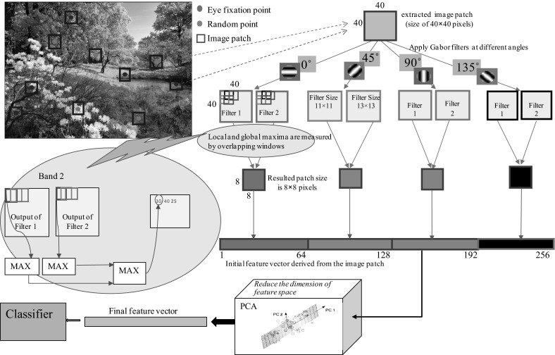
Visualizing the method of feature vector extraction. First, patches (areas around the eye fixation and random points of the image) are extracted. Second, each image patch is convolved with two Gabor filters with filter sizes of 11 × 11 and 13 × 13 and for four orientations independently. These units play the role of the V1 simple cells. For each orientation that contains two simple maps, the complex unit responses are computed by subsampling these maps using a window of size 10 × 10 pixels that from each window, one single measurement is obtained by taking the maximum of all 100 elements. Because the size of the extracted original patch is 40 × 40 pixels, a patch with the size of 8 × 8 pixels is created for every one of the four orientations. Finally, a feature vector of length 256 is obtained for this sample image patch. Finally, the PCA algorithm is used in order to reduce the dimensionality of the features space
In this method, the free parameters are the “patch size” and the “number of components” in PCA. First, we selected the number of the PCA components that contained more than 90 % of the total variance in input data (initial feature vector space). After calculating and plotting the PCA eigenvalue spectrum it was found that, first 18 principal components have more than 90 % of the total variance in the input data. We calculated the PCA eigenvalue spectrum for the extracted patches with different sizes (30 × 30, 40 × 40, 50 × 50, 60 × 60 and 80 × 80 pixels), and the results showed that the first 18 principal components include the 90 % of the total variance in input data. Therefore, we have a feature vector of length 18 for every image patch (with any size) hereinafter. For instance, assuming that the average number of fixation points for each image is six (equivalent the six fixation patches), thus for each image there is also a six control points and totally there are twelve feature vectors for each viewed image. With these assumptions, because each individual see 108 images, all data related to a person will be equal to 1296 feature vectors (108 images × 12 patches).
Adding spatial frequency as another feature
In order to increase the accuracy of classification to separate the fixation and non-fixation locations in previous section, we looked for another feature that is quite different between the two locations (in addition to the extracted orientations). This feature is a measure of the spatial frequency of the image patches. The experimental evidence have shown that the visual cortex neurons respond more robustly to sine wave gratings that are placed at particular angles in their receptive fields than they do to edges (Shi et al. 2011). Indeed, most neurons in the V1 area of the visual cortex have the best response when a sine wave grating of a specific frequency is presented at a particular angle in a particular location in their visual field (Issa et al. 2000; Martinez and Alonso 2003). In this case, the spatial frequency is a measure of how often sinusoidal components of the structure repeat per unit of distance. The spatial frequency is expressed as the number of cycles per degree of visual angle.
To calculate and obtain a measure of the patches’ spatial frequency, first we applied the 2D-DFT on each image patch (such as “Spatial frequency” section, spatial frequency for image). The number of Fourier coefficients that their amplitude is larger than a threshold value was calculated for each of the image patches separately, as a measure of the spatial frequency of the image patch. We considered the threshold value equal to the average amplitude of the Fourier coefficients for each image patch separately (Fig. 8). Finally, this measure was normalized to the number of all the Fourier coefficients of each patch.
Fig. 8.
Calculating a measure of the spatial frequency where green circle shows fixation point and blue circle shows non-fixation point (control point). (Color figure online)
In the next step, the spatial frequency feature (as a one-dimensional feature) added to the feature vector obtained from the orientations and by applying the PCA algorithm for each image patch.
Training different statistical classifiers
After extracting the feature vectors for all fixation and non-fixation patches for each of the images seen by any individual separately, we labeled these patches. The fixation patch label was set to be equal to “1” and the control patch label was selected to be equal to “0”. In order to specify a label for each test image patch (fixation patch label = 1, non-fixation patch label = 0), we take the advantage of a classifier. To evaluate the model, we used the technique of repeated random sub-sampling validation. This method randomly splits the dataset into training and validation data. For each such split, the model is fitted to the training data and predictive accuracy is assessed using the validation data. Then, the results are averaged over the splits. So after extracting all feature vectors for each of images seen by any individual, feature vectors corresponding to 80 % of the observed images (all images include the natural and man-made scenes; 29 images × 3 blocks of the trials = 87) were considered randomly as the training data. The classifier trained using these data. Feature vectors corresponding to 20 % of the outstanding images 21 images were considered as the test data and classification of these data will be evaluated. Breaking the data into two parts training and test was performed 20 times randomly and we reported the average classification accuracy for this 20 times for the data related to each person separately. The same process was performed on the data belonging to all individuals participated in the experiment and at the end, this accuracy was averaged across all individuals. We used four classifiers in classification step: Naive Bayes, K-nearest neighbor, Support Vector Machine with radial basis function as kernel functions (RBF-SVM) and linear Support Vector Machine.
Results
The result of the average classification accuracy is calculated in this section. Free parameters of this method include the image patch size. Therefore, performance was measured for different sizes of the extracted patches.
Average classification accuracy
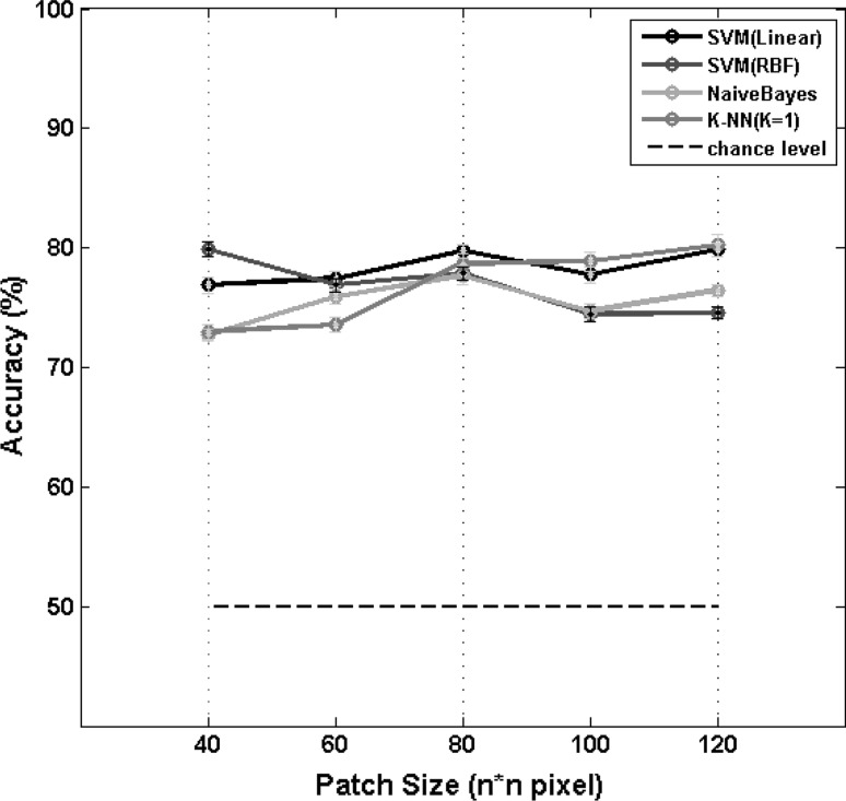
The results of the average classification accuracy in across all subjects are shown in Fig. 9. As can be seen in the figure, K-nearest neighbor classifier for image patches with a size of 120 × 120 pixels has the highest accuracy (80.23 ± 0.92 %). Also, support vector machine with radial basis kernel function (79.94 ± 0.62 %), linear support vector machine (79.84 ± 0.5 %) and Naive Bayes (77.72 ± 0.78 %) classifiers for image patches with a size of 40 × 40, 120 × 120 and 80 × 80 pixels have the highest accuracy respectively (reported values are: averaging the performance across all subjects ± the standard error of the mean).
Fig. 9.
The mean accuracy of different classifiers for prediction of eye fixation points for orientation and spatial frequency as features, depending on the sizes of the patches extracted from the images. Values are based on averaging the accuracy of the data relating to 14 subjects and the error bars indicate the standard error of the mean across all subjects (±SEM)
It should be mentioned that, we performed the same random subsampling validation method in before adding the spatial frequency feature condition. The average of classification accuracies over 14 individuals for patches with sizes of 40 × 40, 60 × 60, 80 × 80, 100 × 100 and 120 × 120 pixels was calculated. The K-nearest neighbor classifier for image patches with the size of 120 × 120 pixels has the highest accuracy (76.5 ± 0.99 %). Also, SVM with radial basis kernel function (76.34 ± 0.49 %), linear support vector machine (76.28 ± 0.51 %) and Naive Bayes (74.84 ± 0.71 %) classifiers for image patches with a size of 40 × 40, 120 × 120 and 80 × 80 pixels have the highest accuracy respectively (reported values are: averaging the performance across all subjects ± the standard error of the mean). This means that classification accuracies have been increased between 3 and 4 % by adding the image patches’ spatial frequency features.
Pooling all subject’s data and create the saliency map
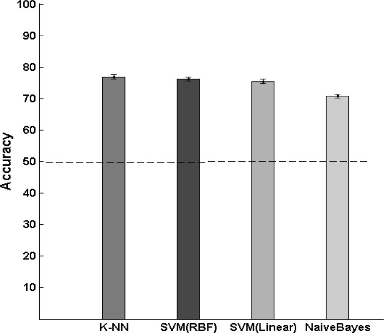
In this section we pooled the data across all subjects and then we utilized the Repeated Random Sub-sampling (RRS) method (splitting the dataset into training and validation data randomly) in order to evaluate the performance of the classifiers. Total number of the image patches was equal to 16,730 for the data relating to all subjects (8365 fixation image patches and 8365 control image patches). Therefore, classifiers were trained with 13,384 image patches and were tested with the remaining 3346 image patches. The RRS method was implemented for 30 times on the data of all the subjects. In this case the image patches with size of 80 × 80 pixels were used because all classifiers were in good agreement in this size (Fig. 9). In addition, no significant difference in the classifiers performance of this size was seen as compared with the maximum performance for other sizes. In order to decrease the run time of the algorithm, we do not want to use large sizes. The results of the average classification accuracies are shown in Fig. 10. The K-nearest neighbor classifier has the highest accuracy equal to 76.9 ± 0.6 %. In addition, support vector machine with radial basis kernel function has accuracy of 76.2 ± 0.73 %. Linear support vector machine and Naive Bayes classifiers have the accuracy of 75.4 ± 0.66 and 70.8 ± 0.71 % respectively (reported values are: averaging the performance across thirty times of running the RSS algorithm ± the standard error of the mean).
Fig. 10.
The results of the average classification accuracy as we pool the data from all subjects for four different classifiers. The image patches size was selected to be 80 × 80 pixels. Error bars indicate the standard error of the mean across all the number of iterations to run the RRS method. Dash line indicates the chance level
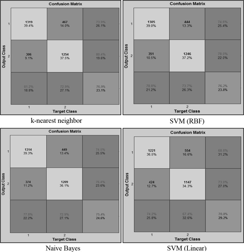
In addition, we calculated the confusion matrices for each of the four classifiers. The results were obtained by averaging over thirty times splitting the data into train and test portions with RSS method. A confusion matrix allows visualization of the performance of classifiers that was represented by a matrix that each row represents the instances in a predicted class, while each column represents the actual classes (Fig. 11). The cells in the confusion matrix include the True Positives, False Positives, False Negatives and True Negatives portions. Assuming that class “1” is the same class of fixation patches and class “2” is the class of control patches, it can be seen from Fig. 11 that performance of the four classifiers is more in class “1” rather than class “2”. For example, for K-nearest neighbor classifier the average accuracy for class “1” is equal to 81.2 % while the average accuracy for class “2” is equal to 72.9 %. This means that the classifiers predict the fixation locations with higher accuracy rather than control locations and this cause that created saliency map be a little noisy. In order to decrease this noise we proposed a method that is explained in the next section.
Fig. 11.
Confusion matrices for each classifier. The results obtained by averaging over thirty times splitting the data into train and test portions with RSS method
In order to create a saliency map for each test image, at the beginning the overlapping patches from the image were extracted from the starting point of the image to the last one. The overlapping patches size was 80 × 80 pixels (for reasons mentioned earlier) with five pixels shift in X and Y directions. Then the feature vectors created for all extracted patches of the image. The classifier was trained with the data of training images (105 images × 14 subjects = 1470 images) and was tested with the feature vectors corresponding to each patch in the training image separately. The classifier determined the label of each test patch. If the test patch label was equal to “1”, the central pixels of the patch was considered to be white in the corresponding saliency map otherwise (label is equal to “0”) all pixels of the patch were considered black (Fig. 12). According to the results of the previous sections, the K-nearest neighbor classifier showed the highest accuracy so we took the advantage of this classifier to create the saliency maps. As can be seen from Fig. 12, the obtained initial saliency map includes the scattered white pixels that are like the salt noises in the images. We have a tendency to remove these pixels because the density of the pixels is very low and so, the probability that these points are the points of fixation of the eye is too low. Indeed, the eyes do not fixate on a limited number of pixels and fixate on an area of pixels in the image.
Fig. 12.
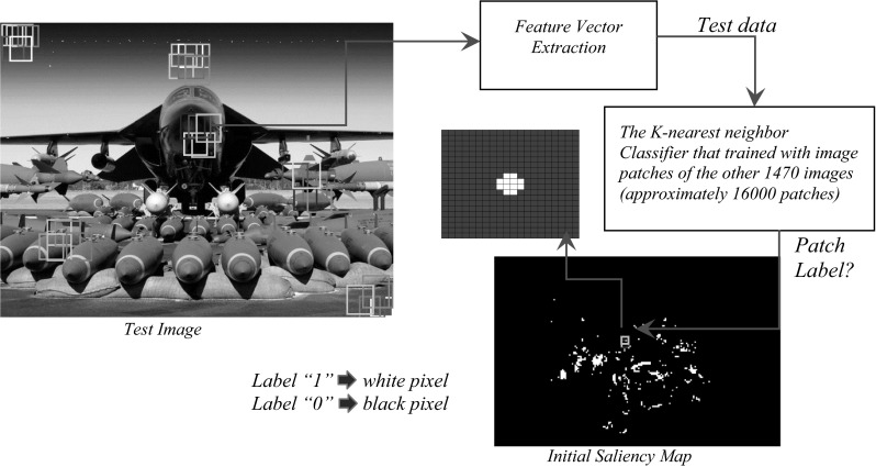
Create an initial saliency map for a sample test image by label of each image patch that specified by the trained classifier
In order to reduce and remove the noise pixels in the saliency map, we trained the classifier with data relating to each subject separately and test the image patches according to the data of each subject independently. Accordingly, 14 labels were determined for each test image patch. The final decision was taken based on voting procedure that predicts the test patch as a fixation point if the patch gets at least 9 votes from the data of 14 classifiers from different subject’s data. By applying this method the noise pixels on the saliency map have been removed well and only the pixels that are dense remains as fixation points. In order to obtain a continuous predicted saliency map for an image, we convolved a Gaussian filter (with filter size = 50 and standard deviation (σ) = 15, we found σ = 15 and filter size = 50 to work well in practice) across the predicted fixation locations in the map resulting of white and black pixels. We also created a continuous human saliency map for each of the images by convolving a Gaussian filter (with the same parameters as before) across the eye tracking data of all subjects in all three blocks for each image.
Performance and evaluation
In this section, we measured the performance of the provided saliency model by its Receiver Operating Characteristic (ROC) curve, for the images used in our experiment and for the Toronto data set (Bruce and Tsotsos 2009). This data set contains data of eye tracking from 20 subjects that have seen the 120 color images of outdoor and indoor scenes (some with very salient items, others with no particular regions of interest) in the free viewing conditions. Images were presented in random order for 4 s each with a gray mask between each pair of images appearing for 2 s. Finally, we compared the performance of our model with the Itti, Koch, and Niebur model (Biologically inspired models, 1998), for the two data sets (Bruce et al. and ours). We used codes which Jonathan Harel (last updated July 24, 2012) has written for Itti and Koch model (http://www.vision.caltech.edu/~harel/share/gbvs.php).
Performance on our data set
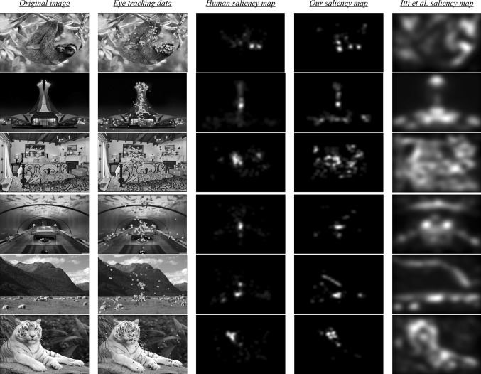
A qualitative comparison of the human saliency map, from eye tracking data, with output maps of Itti et al. model and our model for a variety of test images has been shown in Fig. 13. As can be seen, output saliency maps of our model (the fourth column from the left) are very similar to the actual saliency maps (the third column) than output maps of the Itti et al. model (the last column). Indeed, our model is able to predict properly the possible locations that can be fixated by the subjects. The saliency maps obtained from Itti et al. model includes many of the salient locations and in fact, this model acts on our data set poorly. We intend to evaluate the performance of the two models quantitatively, on test images.
Fig. 13.
A qualitative comparison of the human saliency map, from eye tracking data, with output maps of Itti et al. (1998) model and our model for a variety of test images. From left to right: Original image shown to the subjects. Eye fixation points belonging to 14 viewers in the three blocks of experiment (green, yellow and blue filled circles are corresponding to block 1, block 2 and block 3 respectively). The human saliency map, actual saliency map, computed by convolving a Gaussian filter across the eye fixation points of all subjects in all three blocks (Lighter areas correspond to regions that are more salient). Saliency map as computed by our algorithm. Saliency map as computed by the Itti et al. (1998) algorithm. (Color figure online)
We measured performance of saliency models by their ROC curves. A ROC curve plots the true positive rates as a function of the false positive rates used to present the classification results. In connection with our goal, the ROC analysis is performed between a continuous saliency map that is model output and a set of actual fixation points that are obtained from the eye tracker device. Hit rate (True Positive Rate) is measured in function of the threshold used to binarize the saliency map (Torralba et al. 2006) and (Judd et al. 2009; Hybrid method for comparison). We applied thresholds over the saliency map that are obtained from the models at n = 5, 10, 15, 20, 25, 30, 35, 40, 45 and 50 % of the image for binary saliency maps. For each binary map, we found the percentage of human fixations within the salient areas of the map as the measure of performance. Notice that as the percentage of the image considered salient goes to 100 %, the percentage of human fixations within the salient locations also goes to 100 %.
We apply a threshold to the outputs of the models in order to define predicted regions with a predefined size that allows for comparing the different algorithms. The threshold is set so that the selected image region occupies a fixed proportion of the image size (set to 5, 10, 15, 20, 25, 30, 35, 40, 45 and 50 %). For example, the percent salient 30 % region corresponds to the 30 % of image pixels with higher saliency (in other word, the density is thresholded to select an image region with the highest probability of being fixated that has an area of 30 % of the image size). The efficiency of each model is determined by the percentage of human fixations that fall within the predicted region.
After extraction ROC curves for each test image, we averaged this curves across all images and calculated the area under ROC curve (AUC) for two models, for our data set. The mean of AUC for our model and Itti et al. model was equal to 0.9055 ± 0.0134 and 0.7356 ± 0.0198 (average value for all images ± standard error of mean across images) respectively. The difference was quite significant between the two models (T test: p = 1.64 × 10⁻⁴ and Wilcoxon rank-sum test: p = 1.27 × 10⁻⁴, df = 70). The performance of both models were significantly higher than the chance level (Mean of AUC = 0.55 ± 0.0153). Consider that we have implemented the Itti et al. model when the color channel (C channel) of the model deleted and gray scale images given as inputs to the model. In addition, we have implemented the model with original color images without removing the models color channels that the result presented in the discussion section.
Performance on Toronto data set
In Toronto data set, the mean of AUC for our model and Itti et al. model was equal to 0.7603 ± 0.0127 and 0.7918 ± 0.0134 respectively. This difference was not significant between the two models (T test: p = 0.094 and Wilcoxon rank-sum test: p = 0.073, df = 238). There are two reasons for the reduced performance of our model for Toronto data set than our data set. First, as can be seen from Fig. 14, many of the images used in the Bruce experiment included the regions of interest (ROI) that were created by drastic difference in the color of a particular object with the background of the images. Therefore, it is expected that the performance be less for this data set, because the color feature has not been involved in our model. Second, in the Bruce experiment, each image has been displayed for 4 s whereas this duration was equal to 2 s in our experiment. Indeed, our model is trained with 2 s. It is obvious that subjects observe more locations of the image in duration of 4 s.
Fig. 14.
A few sample images from the Toronto data set. The ROIs created by the difference in color
The discussion and conclusions
In this study, we recorded the eye movements of individuals who view gray scale images of two different semantic categories. Images consisted of natural (e.g., landscape, animal) and man-made (e.g., building, vehicles) scenes. Eye movements of 14 subjects were recorded as they viewed images from two categories in three blocks. In each block, 36 images from two categories (18 images from natural and 18 images from man-made category) were presented randomly to the subjects (overall, each person viewed 108 images). We extracted the fixation locations of eye movements in two image categories by the means of the patches of image that are around the eye fixation points. After extraction of the fixation areas, characteristics of these areas as compared to non-fixation areas were evaluated. In other words, we extracted the features of the fixation locations. These features caused the eyes to be attracted toward those locations. The extracted features include the “orientation” (in the directions of 0°, 45°, 90° and 135°) and “spatial frequency”. After feature extraction phase, different statistical classifiers were trained to predict the eye fixation locations in the new images. The results show that it is possible to predict the eye fixation locations by using the image patches around the subjects’ fixation points. Finally, we obtained the saliency map for images and we compared the output of our model with the Itti et al. model for our dataset and the Toronto dataset. We observed that the performance of our model is much better than Itti et al. model for our dataset. For Toronto dataset the performance of our model decreased slightly (although there was not a significant difference between the performance of the two models). In the “Performance on Toronto data set” section, we mentioned two reasons for the reduced performance of our model for Toronto dataset as compared with our dataset.
We calculated the performance of our model for two categories (natural and man-made scenes) separately. The mean of AUC for natural and man-made categories was equal to 0.8547 ± 0.0233 and 0.9563 ± 0.0172 respectively. The results of prediction for the man-made category was significantly better than the natural one (T test: p = 0.0183 and Wilcoxon rank-sum test: p = 0.0251, df = 34). The results indicate that because we used the “orientation” and “spatial frequency” features for the prediction of eye fixation locations therefore the efficacy of the low-level visual features in attracting the eye movements is affected by the high-level image semantic information. In other words, “spatial frequency” and “orientation” are more effective in attracting the eye movements in the man-made scenes as compared with the natural scenes category.
We do not claim that the model is taken from biological findings completely. In fact, our main concern is of mathematical and computational aspects of the model.
In our experiment, the task of the participants is to report whether the image presented for 2 s is natural or man-made. This is a very easy task given how fast human gist perception is (~100 ms). If we consider very short time for image show (only few milliseconds), then the number of fixations would be so few or even zero (regarding that the first fixation is removed from the analysis and on the other hand, the determination of a minimum time duration of 80 ms for existence of an eye fixation point). In the remaining time, subjects would see the images in a way that they see in free viewing experiment. It seems that eye movements of subjects at the beginning of trial (first 200 ms) is task-dependant and after a time when the subjects perceive the scene, eye movement is similar to free viewing condition and is not task-dependant. All the operations described in the paper can be run at the level of milliseconds after the training phase and so the method described here is suited to artificial detectors.
This point should be considered in this study that whether the difference between the man-made and natural scenes (just two categories) can cover the complex topic of meaning detection and the semantic content of the visual scenes. In another study, we have shown that the pattern of subject’s eye movements are different over the two image categories and this difference has been the effect of semantic contents (As we have controlled the low-level features of the images between the two categories). For this aim we would like to consider images with more semantic contents (categories with different meaning) for our future study (For example considering different semantic contents like sea, forest, and animal etc. for the category of natural images).
Acknowledgments
This research was supported by the School of Cognitive Sciences, Institute for Research in Fundamental Sciences (IPM), Niavaran, Tehran, Iran. We wish to thank Morteza Saraf, Moein Esghaei, Mehdi Behrozi, Kourosh Maboudi and everyone who participated in our experiment.
References
- Awh E, Belopolsky AV, Theeuwes J. Top-down versus bottom-up attentional control: a failed theoretical dichotomy. Trends Cogn Sci. 2012;16(8):437–443. doi: 10.1016/j.tics.2012.06.010. [DOI] [PMC free article] [PubMed] [Google Scholar]
- Bian P, Zhang L. Visual saliency: a biologically plausible contourlet-like frequency domain approach. Cogn Neurodyn. 2010;4(3):189–198. doi: 10.1007/s11571-010-9122-0. [DOI] [PMC free article] [PubMed] [Google Scholar]
- Borji A, Itti L. State-of-the-art in visual attention modeling. Pattern Anal Mach Intell IEEE Trans. 2013;35(1):185–207. doi: 10.1109/TPAMI.2012.89. [DOI] [PubMed] [Google Scholar]
- Bruce ND, Tsotsos JK. Saliency, attention, and visual search: an information theoretic approach. J Vis. 2009;9(3):5. doi: 10.1167/9.3.5. [DOI] [PubMed] [Google Scholar]
- De Valois RL, Albrecht DG, Thorell LG. Spatial frequency selectivity of cells in macaque visual cortex. Vis Res. 1982;22(5):545–559. doi: 10.1016/0042-6989(82)90113-4. [DOI] [PubMed] [Google Scholar]
- De Valois RL, William Yund E, Hepler N. The orientation and direction selectivity of cells in macaque visual cortex. Vis Res. 1982;22(5):531–544. doi: 10.1016/0042-6989(82)90112-2. [DOI] [PubMed] [Google Scholar]
- DeCarlo D, Santella A (2002) Stylization and abstraction of photographs. In: ACM transactions on graphics (TOG), vol 21, no 3. ACM, pp 769–776
- De Filipe S, Alexandre LA. From the human visual system to the computational models of visual attention: a survey. Artif Intell Rev. 2013;39(1):1–47. doi: 10.1007/s10462-012-9386-3. [DOI] [Google Scholar]
- Geisler WS, Perry JS (1998) Real-time foveated multiresolution system for low-bandwidth video communication. In: Photonics West’98 electronic imaging. International society for optics and photonics, pp 294–305
- Geusebroek JM, Smeulders AWM (2002) A physical explanation for natural image statistics. In: Proceedings of the 2nd international workshop on texture analysis and synthesis (Texture 2002). Copenhagen, Denmark, pp 47–52
- Gu Y, Liljenström H. A neural network model of attention-modulated neurodynamics. Cogn Neurodyn. 2007;1(4):275–285. doi: 10.1007/s11571-007-9028-7. [DOI] [PMC free article] [PubMed] [Google Scholar]
- Henderson JM, Brockmole JR, Castelhano MS, Mack M (2007) Visual saliency does not account for eye movements during visual search in real-world scenes. In: van Gompel R, Fischer M, Murray W, Hill RW (eds) Eye movements: a window on mind and brain. Elsevier, Oxford, pp 537–562
- Issa NP, Trepel C, Stryker MP. Spatial frequency maps in cat visual cortex. J Neurosci. 2000;20(22):8504–8514. doi: 10.1523/JNEUROSCI.20-22-08504.2000. [DOI] [PMC free article] [PubMed] [Google Scholar]
- Itti L, Koch C. Computational modeling of visual attention. Nat Rev Neurosci. 2001;2(3):194–203. doi: 10.1038/35058500. [DOI] [PubMed] [Google Scholar]
- Itti L, Koch C, Niebur E. A model of saliency-based visual attention for rapid scene analysis. IEEE Trans Pattern Anal Mach Intell. 1998;20(11):1254–1259. doi: 10.1109/34.730558. [DOI] [Google Scholar]
- Jaimes A, Pelz JB, Grabowski T, Babcock JS, Chang SF (2001) Using human observer eye movements in automatic image classifiers. In: Photonics west 2001-electronic imaging. International society for optics and photonics, pp 373–384
- Judd T, Ehinger K, Durand F, Torralba A (2009) Learning to predict where humans look. In: Computer vision, 2009 IEEE 12th international conference on. IEEE, pp 2106–2113
- Koch C, Ullman S. Shifts in selective visual attention: towards the underlying neural circuitry. Hum Neurobiol. 1985;4:219–227. [PubMed] [Google Scholar]
- Lanyon LJ, Denham SL. Modelling attention in individual cells leads to a system with realistic saccade behaviours. Cogn Neurodyn. 2009;3(3):223–242. doi: 10.1007/s11571-008-9073-x. [DOI] [PMC free article] [PubMed] [Google Scholar]
- Le Meur O (2014) Visual attention modelling and applications. Towards perceptual-based editing methods (Doctoral dissertation, University of Rennes 1)
- Le Meur O, Le Callet P, Barba D, Thoreau D. A coherent computational approach to model bottom-up visual attention. Pattern Anal Mach Intell IEEE Trans. 2006;28(5):802–817. doi: 10.1109/TPAMI.2006.86. [DOI] [PubMed] [Google Scholar]
- Li Z. A saliency map in primary visual cortex. Trends Cogn Sci. 2002;6(1):9–16. doi: 10.1016/S1364-6613(00)01817-9. [DOI] [PubMed] [Google Scholar]
- Marat S, Phuoc TH, Granjon L, Guyader N, Pellerin D, Guérin-Dugué A. Modelling spatio-temporal saliency to predict gaze direction for short videos. Int J Comput Vis. 2009;82(3):231–243. doi: 10.1007/s11263-009-0215-3. [DOI] [Google Scholar]
- Martinez LM, Alonso JM. Complex receptive fields in primary visual cortex. Neurosci. 2003;9(5):317–331. doi: 10.1177/1073858403252732. [DOI] [PMC free article] [PubMed] [Google Scholar]
- Oliva A, Torralba A, Castelhano MS, Henderson JM (2003) Top-down control of visual attention in object detection. In: Image processing, 2003. ICIP 2003. Proceedings. 2003 international conference on (vol 1, pp I–253). IEEE
- Posner MI. Orienting of attention. Q J Exp Psychol. 1980;32(1):3–25. doi: 10.1080/00335558008248231. [DOI] [PubMed] [Google Scholar]
- Rajashekar U, Cormack LK, Bovik AC (2003) Image features that draw fixations. In Image processing, 2003. ICIP 2003. Proceedings. 2003 international conference on (vol 3, pp III–313). IEEE
- Rensink RA, O’Regan JK, Clark JJ. To see or not to see: the need for attention to perceive changes in scenes. Psychol Sci. 1997;8(5):368–373. doi: 10.1111/j.1467-9280.1997.tb00427.x. [DOI] [Google Scholar]
- Riesenhuber M, Poggio T. Hierarchical models of object recognition in cortex. Nat Neurosci. 1999;2(11):1019–1025. doi: 10.1038/14819. [DOI] [PubMed] [Google Scholar]
- Riesenhuber M, Poggio T. Models of object recognition. Nat Neurosci. 2000;3:1199–1204. doi: 10.1038/81479. [DOI] [PubMed] [Google Scholar]
- Schiller PH, Finlay BL, Volman SF. Quantitative studies of single-cell properties in monkey striate cortex: III. Spatial frequency. J Neurophysiol. 1976;39(6):1344–1351. doi: 10.1152/jn.1976.39.6.1334. [DOI] [PubMed] [Google Scholar]
- Schiller PH, Finlay BL, Volman SF. Quantitative studies of single-cell properties in monkey striate cortex. I. Spatiotemporal organization of receptive fields. J Neurophysiol. 1976;39(6):1288–1319. doi: 10.1152/jn.1976.39.6.1288. [DOI] [PubMed] [Google Scholar]
- Schiller PH, Finlay BL, Volman SF. Quantitative studies of single-cell properties in monkey striate cortex. II. Orientation specificity and ocular dominance. J Neurophysiol. 1976;39(6):1320–1333. doi: 10.1152/jn.1976.39.6.1320. [DOI] [PubMed] [Google Scholar]
- Serre T, Riesenhuber M (2004) Realistic modeling of simple and complex cell tuning in the HMAX model, and implications for invariant object recognition in cortex (No. AI-MEMO-2004-017). Massachusetts Inst of tech Cambridge computer science and artificial intelligence lab
- Serre T, Wolf L, Poggio T (2005) Object recognition with features inspired by visual cortex. In Computer vision and pattern recognition, 2005. CVPR 2005. IEEE computer society conference on, vol 2. IEEE, pp 994–1000
- Shen C, Zhao Q. Learning to predict eye fixations for semantic contents using multi-layer sparse network. Neurocomputing. 2014;138:61–68. doi: 10.1016/j.neucom.2013.09.053. [DOI] [Google Scholar]
- Shi X, Bruce ND, Tsotsos JK (2011) Fast, recurrent, attentional modulation improves saliency representation and scene recognition. In: Computer vision and pattern recognition workshops (CVPRW), 2011 IEEE computer society conference on. IEEE, pp 1–8
- Torralba A, Oliva A, Castelhano MS, Henderson JM. Contextual guidance of eye movements and attention in real-world scenes: the role of global features in object search. Psychol Rev. 2006;113(4):766. doi: 10.1037/0033-295X.113.4.766. [DOI] [PubMed] [Google Scholar]
- Viola P, Jones M. Robust real-time object detection. Int J Comput Vision. 2001;4:34–47. [Google Scholar]
- Wang Z, Lu L, Bovik AC. Foveation scalable video coding with automatic fixation selection. Image Processing, IEEE Transactions on. 2003;12(2):243–254. doi: 10.1109/TIP.2003.809015. [DOI] [PubMed] [Google Scholar]
- Wang X, Lv Q, Wang B, Zhang L. Airport detection in remote sensing images: a method based on saliency map. Cogn Neurodyn. 2013;7(2):143–154. doi: 10.1007/s11571-012-9223-z. [DOI] [PMC free article] [PubMed] [Google Scholar]
- Wei H, Ren Y, Wang ZY. A computational neural model of orientation detection based on multiple guesses: comparison of geometrical and algebraic models. Cogn Neurodyn. 2013;7(5):361–379. doi: 10.1007/s11571-012-9235-8. [DOI] [PMC free article] [PubMed] [Google Scholar]
- Yarbus AL (1967) In: Rigss LA (ed) Eye movements and vision (vol 2, no 5.10). Plenum Press, New York
- Yu Y, Wang B, Zhang L. Bottom–up attention: pulsed PCA transform and pulsed cosine transform. Cogn Neurodyn. 2011;5(4):321–332. doi: 10.1007/s11571-011-9155-z. [DOI] [PMC free article] [PubMed] [Google Scholar]
- Zhang L, Lin W. Selective visual attention: computational models and applications. London: Wiley; 2013. [Google Scholar]
- Zhang L, Tong MH, Marks TK, Shan H, Cottrell GW. SUN: a Bayesian framework for saliency using natural statistics. J Vis. 2008;8(7):32. doi: 10.1167/8.7.32. [DOI] [PMC free article] [PubMed] [Google Scholar]


