Abstract
We consider the joint use of spectral and temporal data for multiplexed fluorescence molecular tomography to enable high-throughput imaging of multiple fluorescent targets in bulk tissue. This is a challenging problem due to the narrow near-infrared diagnostic window and relatively broad emission spectra of common fluorophores, and the distortion (“redshift”) that the fluorophore signals undergo as they propagate through tissue. We show through a Cramér-Rao lower bound analysis that demixing with spectral-temporal data could result in an order of magnitude improvement in performance over either modality alone. To cope with the resulting large data set, we propose a novel two-stage algorithm that decouples the demixing and tomographic reconstruction operations. In this work we concentrate on the demixing stage. We introduce an approach which incorporates ideas from sparse subspace clustering and compressed sensing and does not require a regularization parameter. We report on simulations in which we simultaneously demixed four fluorophores with closely overlapping spectral and temporal profiles in a 25 mm diameter cross-sectional area with a root-mean-square error of less than 3% per fluorophore, as well as on studies of sensitivity of the method to model mismatch.
OCIS codes: (170.3880) Medical and biological imaging, (170.6960) Tomography, (170.3010) Image reconstruction techniques, (170.6920) Time-resolved imaging, (170.1580) Chemometrics, (170.3660) Light propagation in tissues
1. Introduction
Fluorescence molecular tomography (FMT) is an optical technique that provides noninvasive, quantitative, three-dimensional imaging of fluorophores in whole animals. In part propelled by advances in fluorescent probe technology in recent years, it is becoming an important tool for preclinical imaging of small animals [1–3]. It has been employed, for example, to image tumors [4] and assess response to anticancer treatment [5] in mice. But unlike microscopy, where high-throughput imaging of multiple fluorescent targets (“multiplexing”) is now routine, multiplexed imaging through bulk tissue in whole animals remains a challenge. Specifically, the narrow (∼200 nm wide) near-infrared “diagnostic window” and relatively broad emission spectra of common organic fluorophores make accurate identification (“demixing”) difficult. Moreover, light experiences a “redshift” as it propagates through tissue due to nonlinear attenuation by tissue chromophores, most notably hemoglobin. An example of this effect, also known as “spectral coloring” [6], is shown in Fig. 1. Here we see that when the wavelength-dependent properties of tissue are taken into account, the spectral signature of the fluorescent dye Alexa Fluor (AF) 750 is shifted towards longer wavelengths (i.e., redshifted) and more closely resembles that of AF 790. The degree of redshifting depends on the position of the fluorophore, which is unknown a priori in FMT, thus making this distortion difficult to predict.
Fig. 1.
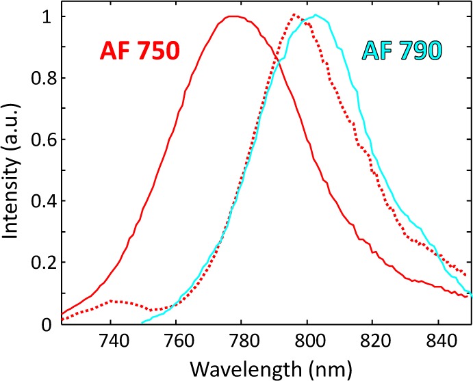
Solid lines: fluorophore spectral signatures for AF 750 (red) and AF 790 (cyan) using data from [7]. Red dotted line: “redshifted” spectrum for AF 750 using optical properties for “skin” in [8] with a distance of ∼20 mm from fluorophore to detector.
However, fluorophores also possess unique temporal signatures, e.g., they have different lifetimes. Some groups have exploited this with time-resolved tomographic instruments to achieve lifetime multiplexing of up to three fluorophores [9, 10]. But recent work in our group suggests that joint measurement of spectral and temporal data can enable robust demixing and localization of four or more concurrent fluorophores [11]. To this end, we are developing a novel time-domain hyperspectral tomographic instrument capable of acquiring time-resolved fluorescence data with 16 spectral channels in the 650-850 nm range. We note that a different system for the acquisition of spectral and temporal data was recently proposed in [12] and used to map the relative concentration of two fluorophores. Because FMT requires many source-detector pair measurements, our instrument generates a large amount of data. In this work, we present a two-stage data processing algorithm that effectively deals with the computational burden created by this large data set. Specifically, we make the following novel contributions:
-
1
We provide a Cramér-Rao lower bound (CRLB) analysis that quantifies the potential performance improvement resulting from the joint use of spectral and temporal data for demixing over either modality alone.
-
2
We present a data processing algorithm that decouples the demixing and tomographic reconstruction operations, thus significantly reducing the computational complexity of FMT with spectral and temporal data. Our algorithm recovers the entire spectral-temporal fluorophore signature in the initial demixing stage, which gives us the flexibility to use, for example, a combination of different time gate data for improved image resolution in the subsequent tomographic reconstruction stage [10, 13–18].
-
3
We propose a demixing strategy that incorporates ideas from the fields of sparse subspace clustering and compressed sensing [19, 20]. We introduced this strategy in [21]. It uses a suitable “library” of fluorophore signatures (measured or modeled) to compute a nonnegative least-squares (NNLS) estimate of each fluorophore signal in the sample. The algorithm does not require a regularization parameter, even when the library is rank-deficient. We accomplish this by pairing a properly constructed library with the gold standard algorithm for solving NNLS problems [22], and we explain our success by suggesting that this algorithm can be reinterpreted in a surprising way.
As the demixing and tomographic reconstruction stages of the algorithm are independent, we focus here primarily on the optimization and performance assessment of the demixing stage; optimization of the tomographic reconstruction stage is the subject of ongoing work in our group. We note that our demixing approach has the potential to serve as a stand-alone algorithm for other applications that require nonnegative high-dimensional data demixing (e.g., hyperspectral imaging in geophysics [23, 24]).
This paper is organized as follows. In Section 2, we provide a brief description of the instrument, which serves to ground our subsequent discussion of the data model and algorithm. Section 3 outlines the benefits of using joint spectral and temporal data to perform fluorophore demixing and localization. After defining the data model, we present the results of the CRLB analysis. The data processing algorithm is detailed in Section 4, where we also discuss its connections to sparse subspace clustering and compressed sensing. We describe the simulations conducted to validate the algorithm, which include the effect of model mismatch, in Section 5. Our results are presented in Section 6, and we conclude in Section 7 with some observations and ideas for future work.
2. Instrument
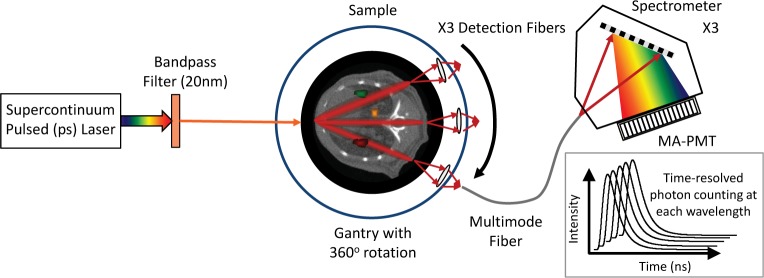
A schematic of the time-resolved hyperspectral tomographic imaging system is shown in Fig. 2. The instrument design and construction will be described more fully in a separate paper; here we provide a brief overview to motivate the algorithm presented in Section 4. (We note, however, that this algorithm could also be applied to spectral-temporal data generated by instruments with other illumination and/or detection schemes.) A pulsed, filtered supercontinuum light source (NKT Photonics) illuminates the sample (phantom or small animal) in a transillumination geometry. The laser wavelength and pulsewidth are 630 nm and ∼30 ps, respectively. The sample is mounted on a rotation stage, permitting illumination over a full 360 degrees. Transmitted and fluorescent light is collected with a set of three long-pass filtered fiber probes mounted on a second rotation stage, so that light can be collected at an arbitrary number of angular positions. The output of each fiber optode is coupled to a spectrograph and 16-channel PMT operated in time-resolved photon counting mode. This allows measurement of time-resolved transmitted fluorescent light as well as transmitted laser light (the “intrinsic measurement”) with 13 nm spectral resolution over the range of 650-850 nm, and with 12 p-s temporal resolution over a 12.5 ns range. Assuming non-overlapping spectral and temporal channels, such a measurement potentially consists of ∼15 × ∼1000 (wavelength × time) samples, and we typically collect ∼650 measurements. In other words, the instrument produces a large data set that uniquely captures both spectral and temporal properties of the emitted light.
Fig. 2.
Schematic of time-resolved hyperspectral tomographic imaging system.
3. Advantages of joint spectral and temporal data
3.1. Data model
We consider a forward model for the FMT problem with joint spectral and temporal data that assumes the following:
-
1
The problem is linear with respect to fluorophore concentration.
-
2
Contributions from each fluorophore are additive.
-
3
Quantum yields, extinction coefficients, lifetimes, and spectra of all fluorophores are known. In other words, the spectral-temporal “signature” of each fluorophore is known; these may be modeled or experimentally measured. We consider relaxing this assumption in Section 5.2.
We further assume that the optical properties of the background medium (assumed infinite and homogeneous) and instrument parameters (source/detector coupling coefficients, calibration constants, etc.) are known, so we neglect Born normalization, and that the time-dependent diffusion equation adequately approximates the radiative transfer equation. These latter two assumptions simplify the modeling but are not essential for the proposed algorithm.
In this work, vector and matrix quantities are in lower- and uppercase bold, respectively, while scalar quantities are in italics. We start with an equation that defines the measurement collected (after background subtraction) by a single source-detector pair (located at rs and rd) for a given spectral (λ) and temporal (t) bin due to the presence of a single fluorophore (located at r):
| (1) |
where β is a factor that accounts for the signal level, Gx and Gm denote the excitation and emission Green’s functions, respectively [25], τ is the fluorophore lifetime, and ∆λ and ∆t denote the width of the spectral and temporal bins, respectively. (We have suppressed the dependency of Gx on the excitation wavelength since this is constant across all measurements.) The quantity η(r,λ), sometimes called the fluorescent yield, is defined as
| (2) |
where ε is the extinction coefficient of the fluorophore at the excitation wavelength, c is the fluorophore concentration, Q is the fluorophore quantum yield (at the peak emission wavelength), and M(λ) characterizes the fluorophore emission in the given spectral bin.
We can rewrite Eq. (1) as
| (3) |
with
| (4) |
Now stacking measurements from all source-detector pairs and spectral-temporal bins, discretizing the imaged volume, and assuming the potential presence of multiple fluorophores, we obtain
| (5) |
where k identifies the particular source-detector pair, J is the Jacobian or weight matrix (i.e., the sensitivity function of the forward problem), and c is the (unknown) fluorophore concentration vector. The matrix J and vector c have the following structure:
| (6) |
| (7) |
| (8) |
with ⊗ symbolizing convolution over time and integration over wavelength and time, as in Eq. (3); J(λ,t) being the Jacobian defined in Eq. (4) for all source-detector pairs and locations r; [E]i,j denoting the (ith, jth) element of the matrix E; and ∆v denoting the volume of the voxel into which the problem has been discretized. The dimensions of the variables are: m is KLT × 1; J is KLT × PF; E is LT × F; and c is PF × 1. Here K denotes the total number of source-detector pairs, L is the number of spectral bins, T is the number of time bins, P is the number of pixels/voxels to be reconstructed, and F is the number of fluorophores potentially present. The dimensions of J here will typically be prohibitively large, so in Section 4.1, we explore a factored way of computing c. An additional drawback of this formulation is that J is no doubt ill-conditioned (if not underdetermined) and so will have to be regularized. This regularization will affect the spectral-temporal demixing operation of any single-step solution as well.
3.2. Cramér-Rao lower bound analysis
The CRLB considered here defines the best theoretical precision (i.e., lowest variance) of any unbiased estimator for a given data model and has long been used in the statistical signal processing community – especially in the radar and sonar signal processing communities – to perform feasibility studies. The basic idea is that the curvature of the log-likelihood function of the data model determines the accuracy with which an unknown (e.g., fluorophore concentration) may be estimated. Log-likelihood functions that are sharply peaked about the unknown quantity permit a more accurate estimate of its value, while the reverse is true for log-likelihood functions that are rather flat in the neighborhood of the unknown. The CRLB provides a measure of this curvature. For a vector of unknowns, it is computed by first calculating the Fisher information matrix, which consists of second derivatives (and first derivative cross products) of the log-likelihood function with respect to each unknown, and then taking its inverse. An introduction to the CRLB is provided in [26]. Here we employ the CRLB to explore demixing performance differences obtainable from three types of data: spectral-temporal, spectral-only, and temporal-only. Because the CRLB is algorithm-independent, it permits us to assess the impact of the data types themselves on theoretically attainable accuracy.
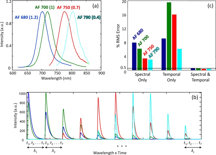
Consider a simpler version of the problem defined by Eq. (5), where the distribution of the fluorophores is assumed known. In other words, this is now simply a demixing problem as tomography for localization is unnecessary. We assume that there are four common fluorophores from the Alexa Fluor series present in our measurement: AF 680, 700, 750, and 790. Their emission spectra and lifetimes, along with their spectral-temporal signatures, are shown in Figs. 3(a) and 3(b). These signatures were generated from data in [7] by assuming the following instrument parameters: an excitation wavelength of 670 nm; a spectral range and resolution of 700-850 nm and 15 nm (10 spectral channels in total); and a temporal range and resolution of 0-7.5 ns and 10 ps (750 temporal channels in total). The background optical properties were µa = 0.7 cm−1 and , typical of those encountered in small animal imaging [8], and the source and detector were located 12.5 mm away from the fluorophore on opposite sides. In this case, the dimensions of J are 7500 × 4, since there is only a single measurement (LT = 7500) and F = 4. Our spectral-temporal data model is
| (9) |
Fig. 3.
(a) Emission spectra and lifetimes (in ns in parentheses) for four common fluorophores: Alexa Fluor 680, 700, 750 and 790; data from [7]. (b) Spectral-temporal signatures associated with each fluorophore; each two-dimensional signature was concatenated into a vector. (c) Cramér-Rao lower bounds for root-mean-square (RMS) demixing error for three data types with all four fluorophores present. Lower values indicate better performance.
where we have written instead of J to represent this smaller full-rank matrix, c in this case is a 4 × 1 vector denoting the concentration of each fluorophore (assumed constant over the known distribution), and n is a vector of independent Poisson noise. We can generate spectral-only and temporal-only data from this model by summing over the time and wavelength bins, respectively. The CRLB for the variance of the elements of c is given by the diagonal of the matrix
| (10) |
where [*]T denotes the transpose, and R is a diagonal covariance matrix containing the mean of the measurements on its diagonal (i.e., ) [27]. In other words, if σ2(ci) represents the variance of the estimate of the concentration of the ith fluorophore generated by an unbiased estimator, then σ2(ci) ≥ [CCRLB]ii. We set the maximum signal-to-noise ratio (SNR) of each fluorophore to 30 dB for the three data types prior to computing CCRLB. Since the CRLB presented here is for unbiased estimators, the variance is equivalent to the mean squared error. Therefore, by taking the square root, we obtain the lower bound on the root-mean-square error of the concentration estimate. In Fig. 3(c), we display this as a percent of the concentration. We see that with joint use of spectral and temporal data, there is roughly an order of magnitude improvement in the lower bound on precision compared to spectral- or temporal-only. We note that slightly worse performance is seen with AF 680 and AF 700 vs. AF 750 and AF 790, since the former two have very similar spectral emission profiles and lifetimes. Similar trends indicating the superiority of spectral-temporal data over either modality alone for the demixing problem have recently been experimentally observed in our lab [11].
Since the FMT problem is ill-posed, we cannot compute the CRLB for it without applying additional restrictions, as discussed in [28]. However, it has been shown by our group and others [10, 13–18] that information from different time gates can be used to improve the resolution of tomographic reconstructions, so having access to temporal data (with or without spectral data) for FMT would appear to be an advantage. With respect to demixing, however, temporal-only data resulted in performance that was at times significantly worse than the other two modalities (e.g., AF 700 and AF 750 in Fig. 3(c)). We note that the CRLB analysis presented in this section holds when the fluorophore signatures – and hence, the spectral properties of the background (whether constant or wavelength-dependent) – are known. An analysis that takes into account errors in the assumed signatures due to imperfect knowledge of the background properties is a significant undertaking in its own right and beyond the scope of the present paper.
4. Algorithm
4.1. Two-step solution: first spectral-temporal demixing and then FMT
As noted above, the time-domain hyperspectral tomographic instrument produces a very large data set, making the direct solution of Eq. (5) at best impractical. Moreover, since the FMT problem is ill-posed and the spectral-temporal demixing problem may not be (or may be less so), it seems reasonable to try to implement an optimal solution for the latter before attacking the former, as in this way we avoid contaminating the demixing problem with errors due to regularization in FMT. This idea of limiting the impact of regularization was used in [29], albeit in a different way, to preserve the spectral prior information for the spectrally-constrained diffuse optical tomography problem. With this in mind, we propose a two-stage algorithm, wherein we first demix each source-detector pair measurement independently and accumulate the measurements for each fluorophore, and then do separate FMT reconstructions to obtain “concentration maps” (cf(r)) for each fluorophore. A flowchart of the algorithm is displayed in Fig. 4. Notice that the two-stage structure gives us the flexibility to employ different tomographic reconstruction algorithms in Stage 2.
Fig. 4.
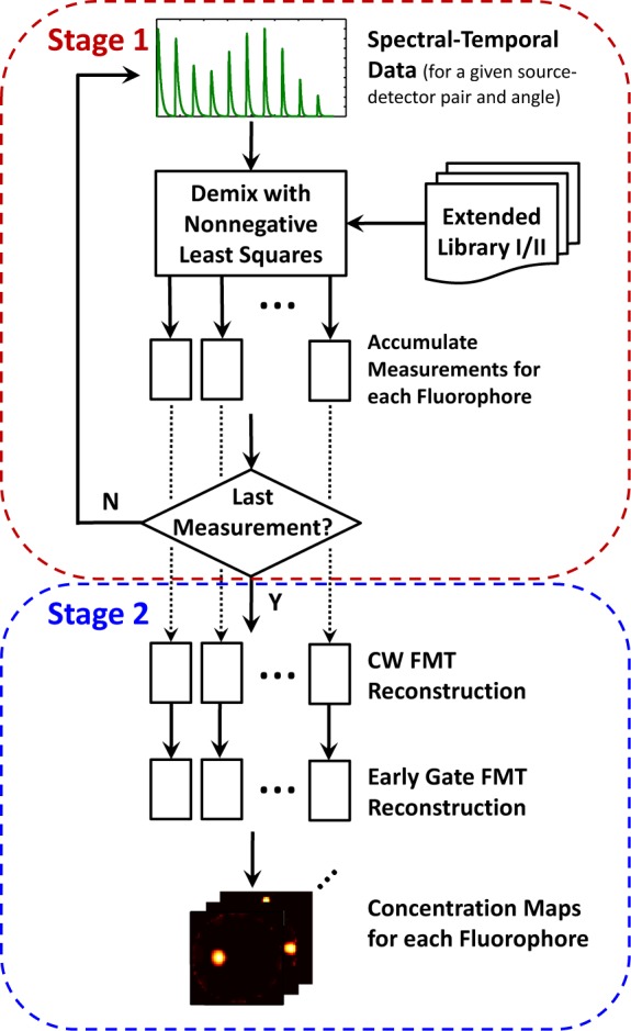
Data processing algorithm flowchart. Demixing of each source-detector pair measurement is accomplished in Stage 1; tomographic reconstructions for each fluorophore are performed in Stage 2.
We employ a traditional linear mixing model for our measurements. Specifically, we write the individual source-detector pair measurement as follows:
| (11) |
with
| (12) |
and
| (13) |
where mk denotes the spectral-temporal measurement for the kth source-detector pair and is of size LT × 1; the columns of S (the “library”) contain the fluorophore spectral-temporal signatures, and Sf is of size LT × N, where N is the number of signatures associated with each fluorophore; ak is of dimension FN × 1 and contains the combining coefficients for the kth source-detector measurement; and n is a vector of independent Poisson noise. The number of columns in S depends on the particular library selected, which we discuss in the following section. For now, observe that when N = 1, we have the data model defined in Eq. (9).
We solve for ak using Matlab’s “lsqnonneg” function (MathWorks, Natick, MA, USA), which implements Lawson and Hanson’s nonnegative least-squares (LH-NNLS) algorithm [22]. In particular, this algorithm solves
| (14) |
where means that no component of ak is negative. Once ak has been determined, we recover the contribution to mk from the f th fluorophore by computing
| (15) |
For the case of N = 1, the constraint is necessary in order to satisfy Assumption 2 in Section 3.1 (“contributions from each fluorophore are additive”), since each component of ak corresponds to a different fluorophore. When N > 1, this constraint can be relaxed to , i.e., linear combinations corresponding to different fluorophores are nonnegative. However, since every element of S is nonnegative, ensures , so we use the more stringent constraint. We found that it worked well in practice and several well-tested algorithms exist for the NNLS problem.
The set of all such source-detector measurements for each fluorophore (mk(f) for k = 1 to K) then becomes the input to a single-fluorophore FMT problem (Stage 2 of the algorithm). We may sum these over wavelength and time and solve a quasi-continuous wave FMT problem, or we could use a combination of time gates to improve the resolution of our reconstructions, as in [13]. An advantage of this formulation is that the number of FMT problems to solve is F, typically ≤ 5, and demixing via LH-NNLS is comparatively quick – we demixed 648 measurements on a laptop in ∼5 min, and faster versions of this algorithm are available (e.g., [30]). We note that even when S is rank-deficient (or at best ill-conditioned), which happens when N is large, we still obtain very good results with LH-NNLS, despite the absence of a regularization parameter in Eq. (14). The reasons for this are discussed in Section 4.3.
4.2. Libraries: naive and extended
According to Eq. (11), the measured fluorophore signal can be approximated as a linear combination of the columns of the library, S. Here we describe the construction of S for three different scenarios. The difference between them depends on whether the positions of the fluorophores are assumed known and on the degree of redshifting believed to be occurring in the sample. The overarching principle, however, is to include in the library a sufficient number of signatures to capture the expected variability of the measured signal. We first describe the construction of S for the simplified model assumed in Section 3.1 and later comment on the generalizability of the approach.
Given the assumptions in Section 3.1, we see that Gx and Gm in Eq. (1) must be the time-dependent Green’s functions for an infinite homogeneous medium. Therefore, for a given fluorophore in a medium with a given absorption (µa(λ)) and reduced scattering coefficient , the fluorophore’s signal at rd depends on ║r−rs║ and ║r−rd║, i.e., its distance to the source and to the detector. This means that for the FMT problem, it is impossible to associate only one signature with each fluorophore as we did in Section 3.2, when we assumed that the fluorophore positions were known. We refer to S defined in this manner, with N = 1, as the “Naive Library.”
When the absorption and reduced scattering coefficients are assumed constant and equal at the excitation and emission wavelengths (the case of no redshifting), the shape of the fluorophore signal depends only on the sum of its distance to the source and detector – in other words, on the total pathlength. A map of total pathlengths for a source-detector pair is shown in Fig. 5. In this case, we are able to decrease the demixing error by including in S multiple signatures of different total pathlengths for each fluorophore. For the particulars of our situation (e.g., source-detector configuration, sample size, optical properties, etc.), which we discuss in Section 5, simulations revealed that total pathlengths of 23, 25, and 27 mm for each fluorophore were sufficient to keep the demixing error down to ~1%. (See Section 5.1 for the definition of the error metric.) We refer to this pathlength-dependent library, with N = 3, as “Extended Library I.” While the precise value of N will vary depending on the imaging system and requirements on the demixing error, the central idea is that only total pathlength (and not the individual distances to the source and detector) need be considered when the dependence of µa and on wavelength is expected to be negligible. This leads to a library with full column rank and an overdetermined least-squares demixing problem.
Fig. 5.
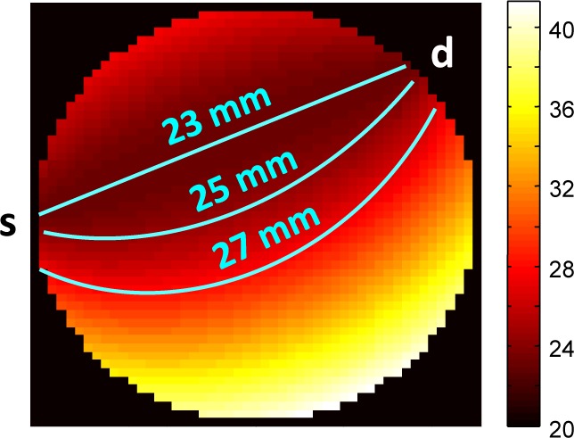
Distribution of pathlengths (mm) for nearest source-detector pair. Color indicates sum of distance to source (s) and detector (d) from that location; lines show where that sum equals 23, 25, and 27 mm.
When the absorption and reduced scattering coefficients vary more strongly with wavelength (resulting in redshifting), the individual distances to the source and detector become important, as the amount of redshifting we measure is proportional to ║r−rd║. An example of this is shown in Fig. 6, where we plot the spectral-temporal signature of AF 680 as a function of position in the sample. In all the three cases, the total pathlength is the same (25 mm), but the amount of redshifting increases with increasing distance to the detector (i.e., as we go from “close to detector” to “midpoint” to “close to source”). In this case, we employed the following steps to arrive at a library. For each fluorophore:
-
1
Generate signatures for all source-detector pairs and a dense set of fluorophore locations within the sample (i.e., at each pixel/voxel location).
-
2
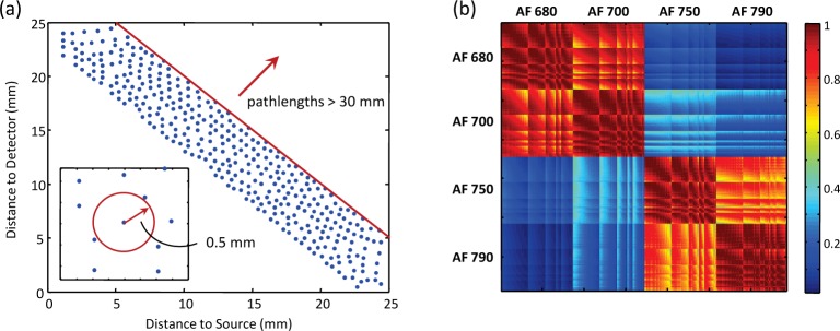
Prune signatures with total pathlengths greater than some value, which in our case we set to 30 mm (see Fig. 7(a)). This value represents a distance from the source and detector so large that fluorophores at such locations would have a negligible impact on the measured signal at that detector.
-
3
Prune signatures such that no two correspond to fluorophore locations whose distance to the source and detector differ by less than some value, which in our case we set to 0.5 mm, as shown in Fig. 7(a). This value represents a distance so small that the resulting signatures are practically equivalent.
Fig. 6.
Spectral-temporal signature of AF 680 as a function of position in sample (7 of 10 spectral channels shown). Redshifting increases with increasing distance to detector, even if pathlength remains constant at 25 mm.
Fig. 7.
Extended Library II: (a) Sampling locations as a function of distance to source and detector; inset shows minimum distance between samples. (b) Coherence of library, measured as ST S. Note that signatures are normalized to unit norm, as explained in text.
We refer to this library, with N = 344, as “Extended Library II,” and with such a library our demixing error was ∼2%. As in the previous case, the particular parameters used to prune the library will depend on the specifics of the imaging system and desired demixing error, but the goal is to include enough signatures for each fluorophore to capture the potential diversity of the measured signals. Such a library contains blocks of highly correlated signatures (see Fig. 7(b)), and the resulting matrix S is no longer full-rank. Nevertheless, we are still able to arrive at a good solution with LH-NNLS, for reasons discussed in Section 4.3.
Although we used a simplified signal model to generate the contents of the library in all three cases, a more complex forward model is a viable alternative, as the library does not change from measurement to measurement and would typically be generated offline. Additional possibilities include a hybrid model-data approach (i.e., a model with some experimentally measured parameters) or signatures derived completely from laboratory measurements. Note that only the shapes of the signatures in the library are important, as their magnitude can be subsumed into the scale factor ak. This is because we attach no physical significance to the magnitude of the components of ak; we care only that when used as combining coefficients with the proper vectors, they result in a good approximation of the underlying fluorophore signal(s). Therefore, we normalize the columns of S to have unit norm.
4.3. Connections to sparse subspace clustering and compressed sensing
In this section, we provide some intuition behind the success of LH-NNLS when the library S is rank-deficient. For our specific problem, mathematical proofs of the results we mention are not available, and we leave that to future work. Nevertheless, there have been recent developments in sparse subspace clustering and compressed sensing that allow us to reinterpret the demixing problem with Extended Library II in ways that provide some insight. As one might expect, when S is rank-deficient, the solution vector ak is not uniquely defined. But in contrast to many least-squares problems, where the goal is to recover ak, we are only interested in Sf ak,f for each k,f – i.e., we do not care about the components of ak per se, but only that Sf ak,f well-approximates the k,f th fluorophore signal. This is a less demanding problem that we are able to solve by relying on two additional insights.
First, we can reinterpret S in Eq. (12) as a union of subspaces, with each section Sf defining the subspace corresponding to the f th fluorophore. Given this interpretation, recent work in sparse subspace clustering demonstrates that if a given vector y lies close to subspace Sf (contained in S), then a sparse solution of is zero outside of the components corresponding to the columns of Sf [19, 31–33]. In other words, y can be expressed as a linear combination of columns only from Sf, which is the assumption inherent in Eq. (15) that makes recovery of the underlying fluorophore signals possible. This property is termed “self-expressiveness” in [19] and “exact feature selection” in [31]. For us, feature selection is not exact but approximate – our solution has small nonzero components from other subspaces – and occurs only if sparsity is coupled with a nonnegativity constraint on ak. In this case, the demixing error is very small and has a negligible impact on the subsequent tomographic reconstructions of fluorophore concentration. We note that this sparsity constraint does not require the fluorophores themselves to be sparsely distributed within the sample, as verified by our simulations in Section 5.
It is perhaps not widely appreciated that nonnegativity itself can, under certain circumstances, be enough to regularize an underdetermined problem [34–37]. In our case, given the highly coherent Extended Library II matrix, nonnegativity alone does not succeed in sufficiently constraining ak. But it does appear to be restrictive enough to cause “approximate feature selection” (AFS) when combined with sparsity, even when the measurement vector is, unlike y, a linear combination of several fluorophore signals that belong to different subspaces. This particular case of AFS given a linear combination of nonnegative signals has not been treated in the literature.
Empirically, we find that enforcing sparsity coupled with the nonnegativity constraint in Eq. (14) is sufficient to ensure successful demixing. And we explain our success with LH-NNLS in this case by reinterpreting it as a nonnegative version of orthogonal matching pursuit (OMP) – our second insight. OMP is a greedy algorithm usually attributed to [38] and popular in the compressed sensing community for obtaining sparse solutions. We are not the first to notice the similarity between LH-NNLS and OMP [39]. But to the best of our knowledge, we are the first to use LH-NNLS directly as a sparsity-promoting solver, thus eliminating the need to specify a regularization parameter. We note that while OMP requires either a maximum number of iterations or the norm of the residual to be specified, which serve as proxies for a regularization parameter, LH-NNLS requires no such stopping criteria. Instead, LH-NNLS checks to see if the Karush-Kuhn-Tucker conditions for the NNLS problem have been satisfied. Therefore, we claim that regularization with LH-NNLS, at least in this application, is intrinsic.
5. Simulations
To test the performance of our algorithm, we conducted simulations that included the effects of noise and model mismatch. In all cases, we simulated the presence of four fluorophores: Alexa Fluor 680, 700, 750, and 790 – see Fig. 3(a) for emission spectra and lifetimes, obtained from [7]. This emission and lifetime information, along with the fluorophores’ excitation profiles, led to the following choice of instrument parameters: an excitation wavelength of 670 nm; a spectral range and resolution of 700–850 nm and 15 nm (10 spectral channels in total); and a temporal range and resolution of 0–7.5 ns and 10 ps (750 temporal channels in total). To simplify the tomographic reconstructions, we considered a two-dimensional problem where the fluorophores, source, and detectors lie in the same plane, but the extension to three dimensions is straightforward. As shown in Fig. 8, we assumed a 25-mm diameter imaging area (typical for small animal imaging) with one source and nine detector locations that rotate around the surface of the sample. The initial source and detector positions were θs = 180 degrees and θd = [−45,−35,−25,−10, 0, 10, 25, 35, 45] degrees, respectively, and the entire source-detector configuration was rotated over 360 degrees, collecting measurements every 5 degrees. This resulted in a total of 648 measurements (9 detectors × 72 locations) each consisting of 7500 components (10 spectral channels × 750 temporal channels).
Fig. 8.
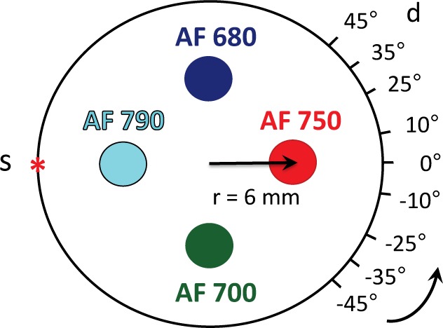
Source-detector configuration and distribution of four fluorophores in sample in “standard positions.” Source (s) and detectors (d) rotate around sample, taking measurements every 5 degrees.
We modeled the fluorophores as both point targets and extended targets; the latter case was in part to test the robustness of the sparsity constraint used with Extended Library II. The extended targets were modeled as disks with a diameter of 3 mm. To ensure that SNR was not the dominant factor in demixing performance, we initially placed all four fluorophores at r = 6 mm from the center of the sample and scaled the peak value from all measurements to 1000 counts for each fluorophore. Given our Poisson noise model, this resulted in a maximum SNR of 30 dB (~3% noise) and an average SNR of ~18 dB (~13% noise), which are consistent with values measured in our lab. We located AF 680 and AF 700 directly across from one another and did the same for AF 750 and AF 790. With our transillumination geometry, this results in the fluorophore pairs most similar to one another often appearing in the same measurement, which makes the demixing problem more challenging. We refer to this configuration as “standard positions.”
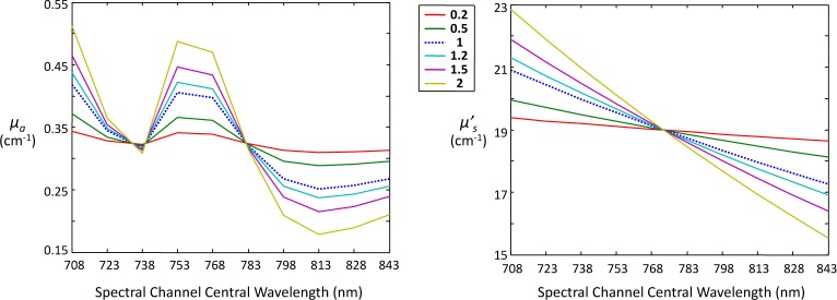
The Naive Library was generated assuming the fluorophores were located at the center of the sample and setting µa = 0.7 cm−1 and , which match the values for “skin” at 670 nm provided in [8]. For Extended Library I, locations resulting in the appropriate pathlengths were selected and the same optical properties were used. Extended Library II used wavelength-dependent values of µa and for each spectral channel for skin [8] to account for redshifting; these values are displayed in blue and labeled as “1” in Fig. 9.
Fig. 9.
Values of absorption (µa) and reduced scattering coefficients per spectral channel for “skin” with scaling constants applied (see text for details). Values labeled “1” (dotted line) reflect the information provided in [8].
5.1. Noise only: with and without redshifting
For the noise-only simulations, fluorophore signals were generated according to Eq. (1), summed, and a vector of independent Poisson noise was added to each measurement. For the case of no redshifting, the absorption and reduced scattering coefficients were assumed constant and equal at the excitation and emission wavelengths and set to µa = 0.7 cm−1 and , as above. To model the effects of redshifting, the wavelength-dependent values of µa and for skin were employed. Ten realizations of each measurement set (648 measurements per set) were demixed, and demixing performance for each fluorophore was assessed by computing the mean and standard deviation of the following error metric over all realizations:
| (16) |
where and Mf denote the matrices containing the demixed signal estimates and true values for all 648 measurements, respectively, and ║·║F signifies the Frobenius norm. This error metric represents a normalized root-mean-square (RMS) error, which we express as a percent in Section 6.
To guard against the possibility of performance with “standard positions” being somehow atypical, we generated 50 realizations of measurement sets (with point targets) where the positions of the four fluorophores in the sample were randomized. We kept the scaling factor (β) in Eq. (1) as before, which meant that the SNR for each fluorophore now varied with radial position. We refer to this group as “randomized positions.”
We also explored the robustness of the demixing algorithm to target size by comparing performance for four extended targets with increasing radii: r = 1.5, 3, 6, and 9 mm. For this comparison, we simulated the presence of AF 680 and used wavelength-dependent values of µa and for skin. We located the targets at the center of the sample and scaled the peak signal value for each to 1000 counts before adding independent Poisson noise. Demixing was performed with Extended Library II. As there was only one target present at a time, the goal here was to evaluate the accuracy of the signal estimates for the varying target sizes as well as the number of significant coefficients in the solution vectors ak (i.e., the level of sparsity of the solution vectors).
Finally, we performed tomographic reconstructions for each demixed fluorophore estimate to assess performance after Stage 2 of the algorithm. We used the method described in [13], which employs a combination of early-arriving photons (EP) and continuous wave (CW) intensity to improve the spatial resolution of the reconstructions. Briefly, as shown in Fig. 4, we performed an initial CW reconstruction and used that result as the starting point for the EP reconstruction. The image reconstructions were obtained with a common algebraic iterative technique, the randomized Kaczmarz method (also known as r-ART) as implemented in [40]. We employed a relaxation parameter of 1.5 along with a nonnegativity constraint and 100 iterations per reconstruction – parameters that were selected empirically to yield stable results of acceptable quality. Our Jacobians were constructed as per Eq. (6); we integrated over all spectral channels, from 0–500 ps for EP and 0–7.5 ns for CW. The range of 0–500 ps corresponds to 3–50% of the peak response, depending on the fluorophore. A pixel size of 1 mm2 was used in all cases.
5.2. Model mismatch due to redshifting
To investigate the sensitivity of our demixing algorithm to mismatch between the contents of the library and the measured input signals, we varied the optical properties of skin used to generate the signals as follows:
| (17) |
where γ is a scale factor whose value ranged from 0.2 to 2 (see Fig. 9), and <·> represents the mean value over all spectral channels. This gave us a way to gauge performance for cases in which the optical properties were, on average, correct, but their precise variation over the spectral channels was either under- (γ > 1) or overestimated (γ < 1) by the library. As above, ten realizations of point-target measurement sets (with noise) were demixed, with all four fluorophores in “standard positions,” and the same error metric was used to characterize performance.
6. Results and discussion
6.1. Fluorophore demixing
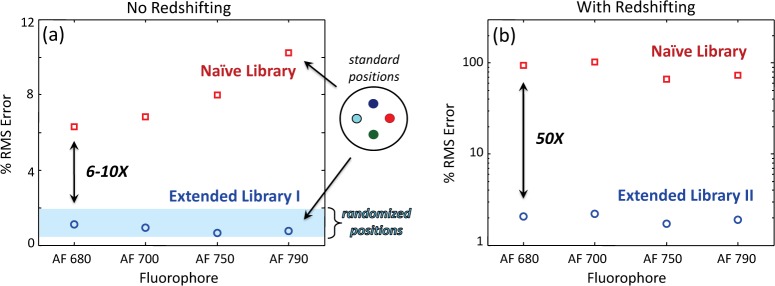
In Fig. 10(a), we display the results of demixing in the absence of redshifting for point targets in both standard (symbols) and randomized (blue background) positions. Standard error bars are not shown as these would be smaller than the symbols. Also, since there was no significant difference from point targets, results for extended targets are omitted for brevity. We draw several conclusions from this figure. First, results from fluorophores in “standard positions” are typical, lying well between the minimum and maximum error values (over all four fluorophores) observed with the randomized positions. Second, the variation in demixing performance due to location in the sample (and hence SNR) is small: ~0.5–2%. Third, approximately a 6–10× performance improvement can be obtained by using Extended Library I instead of Naive Library for demixing. However, tomographic reconstructions generated from both results are indistinguishable by eye (not shown). This agrees with a general trend that emerged from this study: when the demixing error was less than ~10%, the impact on subsequent tomographic reconstructions was negligible. This suggests that when little or no redshifting is expected, accounting for differences in fluorophore signatures due to small differences in pathlengths (~5 mm) is unnecessary for successful FMT reconstructions.
Fig. 10.
Demixing results for none (a) and significant redshifting (b). Values reported are averages of 10 trials; standard error bars are smaller than symbols so not shown. “Randomized positions” represents performance variation over 50 trials with Extended Library I and refers to cases where positions of the four fluorophores in the sample were randomized.
In the presence of significant redshifting, however, accounting for this effect with Extended Library II is crucial, as Fig. 10(b) demonstrates. While performance errors with Extended Library II are below 3%, errors with Naive Library are ~70–100%. This leads to crosstalk and inaccurate fluorophore concentration estimates in the tomographic reconstructions, as discussed in the next section.
Our simulations with extended targets of increasing size revealed no significant difference in the accuracy of the estimated fluorophore signals. Demixing errors here were below 1%, which is consistent with results in Fig. 10(b). (We expect performance to be better with only one fluorophore in the sample versus four.) This demonstrates that our demixing algorithm does not require targets to be sparsely distributed in the sample. With respect to the solution vectors, however, these remain sparse with little change in level of sparsity as a function of target size, as shown in Fig. 11. In this figure, we plot the maximum and average number of significant coefficients in the solution vector ak versus target size. “Significant” is defined here as coefficients within three orders of magnitude of the maximum value of ak. We see that even for a large target (r = 9 mm), the solution vector only possesses ~7 significant coefficients on average, which is just ~2% of the N = 344 signatures in the signal subspace (i.e., the corresponding section of the library). The maximum values for this target were 11 and ~3%. We believe that our solutions remain sparse even as the physical size of the target grows because there is not a one-to-one correspondence between the signatures in the library and different locations in the sample. (Recall that signatures are parameterized in terms of distance to the source and detector, as explained in Section 4.2.) Moreover, the sensitivity function of a given source-detector pair is also spatially limited. However, it is surprising that even a much larger target (r = 9 mm) than the original “extended target” (r = 1.5 mm) can be well-represented by almost the same number of coefficients. Although beyond the scope of the present work, this warrants further investigation.
Fig. 11.

Number of significant coefficients in solution vector ak as a function of target size. Crosses indicate average value (computed over 648 measurement estimates); triangles indicate maximum value. “Fraction” is [number of significant coefficients] divided by 344, which is the total number of signatures in the signal subspace. Target size is quantified in terms of radius (r) and illustrated graphically.
6.2. Tomographic reconstructions
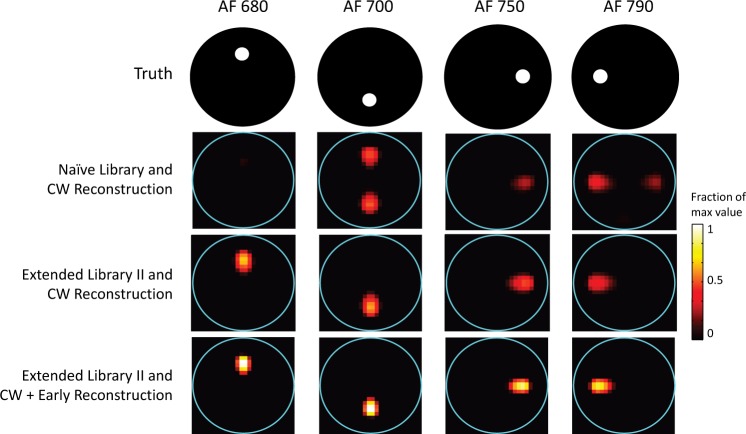
Although the focus of this study was not Stage 2 of the algorithm, it was important to assess the impact of demixing errors on the final tomographic reconstructions. In Fig. 12, we display an example reconstruction for extended targets in the presence of redshifting. For this example, the peak concentration estimate was low by about 30% (compared to the true value), so results have been scaled to this maximum value. (Note that we have made no attempt to optimize this part of the algorithm, and more accurate concentration estimates might be obtained with a different image reconstruction algorithm and/or different algorithm control parameters.) With respect to position, there is very good agreement with truth; the results are slightly biased outward, but only by ~1 mm. In the second row, labeled “Naive Library and CW Reconstruction,” the use of the Naive Library led to demixing errors like the ones displayed in Fig. 10(b), which manifest themselves primarily as significant crosstalk in the reconstructions. In other words, redshifting causes AF 680 to look like the un-redshifted version of AF 700 in the library, and the same occurs for AF 750 with AF 790 (to a lesser degree). With the use of Extended Library II, the demixing error is < 3% and crosstalk is eliminated (third row). Finally, using the CW reconstruction to serve as the starting point for the EP reconstruction results in higher (and therefore more accurate) concentration estimates and slightly sharper reconstructions, demonstrating the advantage of this hybrid approach (fourth row).
Fig. 12.
Tomographic reconstructions of 3-mm diameter fluorescent targets with redshifting.
6.3. Effect of model mismatch
In this work, one of the initial assumptions made to simplify the modeling was that the optical properties of the background medium were known, but in practice, this is rarely the case. As we have seen from comparisons of results with Naive and Extended Library II, not properly accounting for the dependence of µa and on wavelength via the library can have a drastic impact on demixing performance. In Fig. 13, we display the results obtained as the level of mismatch between the library and input fluorophore signals was varied according to Eq. (17). Here the library used for demixing was Extended Library II, but the optical properties employed to generate the fluorophore signals were varied according to γ (see Fig. 9). Cases with γ > 1 correspond to those where the library underestimates the shape of the spectral variation across channels, while those with γ < 1 represent cases where the library overestimates the variation. When γ = 1, there is a match between the assumptions used to generate the library and the signals, and the error is at its lowest, i.e., at the level displayed in Fig. 10(b) for Extended Library II. Interestingly, there is an obvious asymmetry in the results. It seems that overestimating the degree of variation with the library is better than the alternative, presumably since a library incorporating a more pronounced degree of redshifting than is actually present contains a larger diversity of signals, including those from locations near the detectors which experience less redshifting. This suggests that one way of guarding against mismatch might be to intentionally overestimate the degree of variation of the optical coefficients across spectral channels. Another way to mitigate the impact of mismatch (not explored here) may be to employ the Born normalization, which is common in FMT and has been shown to help with model mismatch due to a heterogeneous background [41]. However, this technique may have to be modified in order to account for the spectral range of our measurements.
Fig. 13.

Demixing results in the presence of mismatch between Extended Library II and input fluorophore signals. Legend refers to scale factor (γ) applied to optical properties used to generate signal (see text for details). Values reported are averages of 10 trials; standard error bars are smaller than symbols so not shown.
As previously mentioned, results with demixing error less than ~10% led to good tomographic reconstructions, similar to those shown in Fig. 12, rows 3 and 4. With an error of ~20%, as seen with γ = 1.5, some crosstalk appears in the tomographic reconstructions (not shown). Errors on the order of 50% or higher lead to significant crosstalk, as seen in Fig. 12, row 2.
7. Conclusions and future work
In this work, we considered the advantage of using joint spectral and temporal data for the multiplexed fluorescence molecular tomography problem. Specifically, our goal was to enable high-throughput imaging of multiple fluorescent targets in bulk tissue. This is a challenging problem due to the narrow near-infrared diagnostic window and relatively broad emission spectra of common fluorophores, and the redshift that the fluorophore signals undergo as they propagate through tissue. We showed through a CRLB analysis that the use of spectral and temporal data for demixing could result in an order of magnitude improvement in performance. A similar trend has been observed with data from the time-domain hyperspectral tomographic imaging instrument under development in our lab.
To cope with the significant computational demands of the large spectral-temporal data set, we proposed a two-stage algorithm that effectively decouples the demixing and tomographic reconstruction operations. This approach has the additional benefit that bias resulting from necessary regularization of the tomography problem does not affect demixing. Our demixing algorithm is accurate, comparatively quick, and flexible – it can handle targets of any size and both over- and underdetermined demixing problems without relying on a regularization parameter. By reinterpreting the forty-year-old gold standard algorithm for NNLS and employing a union of subspaces model for the library, we leveraged some recent developments in sparse subspace clustering and compressed sensing to perform demixing under challenging circumstances.
A key component of the demixing algorithm is the use of an “extended library” that allows us to incorporate knowledge about potential signal variability into the problem. As discussed in Section 4.2, for our application demixing strategies where the underlying fluorophore signals are assumed perfectly known are not appropriate, but blind approaches throw away useful information. Our approach strikes a middle ground and is more computationally efficient than statistical algorithms often used to cope with signature (or “endmember”) uncertainties [24]. We used an extended library here to account for signal variability caused by the unknown location of the fluorophore(s) and wavelength-dependent optical properties of tissue, but the same approach might also be employed to account for changes due to the microenvironment (e.g., shifts in fluorophore lifetimes due to pH). We saw that in the presence of significant redshifting, accounting for signal variability was necessary to avoid crosstalk and inaccurate fluorophore concentration estimates in the tomographic reconstructions. Initial analysis suggests that correctly estimating average background optical properties and the general shape of the variation across spectral channels may be sufficient to ensure successful demixing in the presence of strong redshifting.
Our work can be extended along several fronts. Of central importance is the experimental validation of the algorithm, currently in progress. We are evaluating performance with tissue-mimicking phantoms, and these studies will be followed by in vivo animal testing.
Second, the proposed algorithm can be further developed in a number of ways. In the current signal model, we made several simplifying assumptions that may need to be revisited. For example, we ignored fluorophore quenching and saturation effects, the instrument response function and calibration constants, as well as the impact of a heterogeneous background. We also assumed that tissue autofluorescence had been removed by a previous pre-processing step, but it may be possible to incorporate the autofluorescence signal directly into the library of the demixing algorithm. Optimization of the tomographic reconstruction stage of the algorithm is also currently being explored. Particularly attractive are algorithms that make use of time domain data to improve the spatial resolution of the reconstruction (e.g., [13]). Another possibility hinges on the observation that in the presence of redshifting, the demixed signal contains some information about the position of the fluorophore (see Section 4.2). It may be possible to use this information to create a coarse map that could serve as a spatial prior for the tomography problem. (There is some precedent for this in the literature when multispectral measurements are available [42].) As this prior comes directly from the fluorescence signal, it is a better match for our problem than one based on anatomical or structural information. Finally, although results from our initial investigation of model mismatch are encouraging, a more extensive study is needed.
A third direction is the investigation of the limits of what Extended Library II can accommodate in terms of the number of subspaces (i.e., different fluorophores) and their relationships to one another. As mentioned in Section 4.3, our specific problem of AFS given a linear combination of nonnegative (fluorophore) signals has yet to be explored in the literature, and we have not yet succeeded ourselves in a fully mathematical characterization. Work in this area is ongoing. We note that this problem may be relevant to other fields that require nonnegative high-dimensional data demixing.
Acknowledgments
This work was funded by a grant from the National Institutes of Health (R01EB012117).
References and links
- 1.Ntziachristos V., Tung C., Bremer C., Weissleder R., “Fluorescence molecular tomography resolves protease activity in vivo,” Nat. Med. 8, (7)757–760 (2002). 10.1038/nm729 [DOI] [PubMed] [Google Scholar]
- 2.Bai J., Xu Z., “Fluorescence molecular tomography,” in Molecular Imaging: Fundamentals and Applications, Tian J., ed. (Springer, 2013). 10.1007/978-3-642-34303-2_4 [DOI] [Google Scholar]
- 3.Darne C., Lu Y., Sevick-Muraca E. M., “Small animal fluorescence and bioluminescence tomography: a review of approaches, algorithms and technology update,” Phys. Med. Biol. 59, R1–R64 (2014). 10.1088/0031-9155/59/1/R1 [DOI] [PubMed] [Google Scholar]
- 4.Niedre M. J., de Kleine R. H., Aikawa E., Kirsch D. G., Weissleder R., Ntziachristos V., “Early photon tomography allows fluorescence detection of lung carcinomas and disease progression in mice in vivo,” Proc. Natl. Acad. Sci. USA 105(49), 19126–19131 (2008). 10.1073/pnas.0804798105 [DOI] [PMC free article] [PubMed] [Google Scholar]
- 5.Ntziachristos V., Schellenberger E. A., Ripoll J., Yessayan D., Graves E., Bogdanov A., Jr, Josephson L., Weissleder R., “Visualization of antitumor treatment by means of fluorescence molecular tomography with an annexin V-Cy5.5 conjugate,” Proc. Natl. Acad. Sci. USA 101(33), 12294–12299 (2004). 10.1073/pnas.0401137101 [DOI] [PMC free article] [PubMed] [Google Scholar]
- 6.Cox B., Laufer J. G., Arridge S. R., Beard P. C., “Quantitative spectroscopic photoacoustic imaging: a review,” J. Biomed. Opt. 17(6), 061202 (2012). 10.1117/1.JBO.17.6.061202 [DOI] [PubMed] [Google Scholar]
- 7. http://www.lifetechnologies.com/us/en/home/life-science.html
- 8.Alexandrakis G., Rannou F. R., Chatziioannou A. F., “Tomographic bioluminescence imaging by use of a combined optical-PET (OPET) system: a computer simulation feasibility study,” Phys. Med. Biol. 50, 4225–4241 (2005). 10.1088/0031-9155/50/17/021 [DOI] [PMC free article] [PubMed] [Google Scholar]
- 9.Raymond S. B., Boas D. A., Bacskai B. J., Kumar A. T. N., “Lifetime-based tomographic multiplexing,” J. Biomed. Opt. 15(4), 046011 (2010). 10.1117/1.3469797 [DOI] [PMC free article] [PubMed] [Google Scholar]
- 10.Chen J., Venugopal V., Intes X., “Monte Carlo based method for fluorescence tomographic imaging with lifetime multiplexing using time gates,” Biomed. Opt. Express 2(4), 871–886 (2011). 10.1364/BOE.2.000871 [DOI] [PMC free article] [PubMed] [Google Scholar]
- 11.Valim N., “Instrumentation and methods for time-resolved diffuse fluorescence imaging,” Ph.D. Dissertation (Northeastern University, 2014), Chap. 5. [Google Scholar]
- 12.Pian Q., Yao R., Zhao L., Intes X., “Hyperspectral time-resolved wide-field fluorescence molecular tomography based on structured light and single-pixel detection,” Opt. Lett. 40(3), 431–434 (2015). 10.1364/OL.40.000431 [DOI] [PMC free article] [PubMed] [Google Scholar]
- 13.Li Z., Niedre M., “Hybrid use of early and quasi-continuous wave photons in time-domain tomographic imaging for improved resolution and quantitative accuracy,” Biomed. Opt. Express 2(3), 665–679 (2011). 10.1364/BOE.2.000665 [DOI] [PMC free article] [PubMed] [Google Scholar]
- 14.Holt R. W., Tichauer K. M., Dehghani H., Pogue B. W., Leblond F., “Multiple-gate time domain diffuse fluorescence tomography allows more sparse tissue sampling without compromising image quality,” Opt. Lett. 37(13), 2559–2561 (2012). 10.1364/OL.37.002559 [DOI] [PMC free article] [PubMed] [Google Scholar]
- 15.Gao F., Zhao H., Zhang L., Tanikawa Y., Marjono A., Yamada Y., “A self-normalized, full time-resolved method for fluorescence diffuse optical tomography,” Opt. Express 16(17), 13104–13121 (2008). 10.1364/OE.16.013104 [DOI] [PubMed] [Google Scholar]
- 16.Selb J., Dale A. M., Boas D. A., “Linear 3D reconstruction of time-domain diffuse optical imaging differential data: improved depth localization and lateral resolution,” Opt. Express 15(25), 16400–16412 (2007). 10.1364/OE.15.016400 [DOI] [PMC free article] [PubMed] [Google Scholar]
- 17.Hielscher A. H., Klose A. D., Hanson K. M., “Gradient-based iterative image reconstruction scheme for time-resolved optical tomography,” IEEE Trans. Med. Imag. 18(3), 262–271 (1999). 10.1109/42.764902 [DOI] [PubMed] [Google Scholar]
- 18.Hou S. S., Rice W. L., Bacskai B. J., Kumar A. T. N., “Tomographic lifetime imaging using combined early and late-arriving photons,” Opt. Lett. 39(5), 1165–1168 (2014). 10.1364/OL.39.001165 [DOI] [PMC free article] [PubMed] [Google Scholar]
- 19.Elhamifar E., Vidal R., “Sparse subspace clustering: algorithm, theory, and applications,” IEEE Trans. Pattern Anal. Mach. Intell. 35(11), 2765–2781 (2013). 10.1109/TPAMI.2013.57 [DOI] [PubMed] [Google Scholar]
- 20.Candès E. J., Wakin M. B., “An introduction to compressive sampling,” IEEE Signal Process. Mag. 25(2), 21–30 (2008). 10.1109/MSP.2007.914731 [DOI] [Google Scholar]
- 21.Pera V., Brooks D. H., Niedre M., “A sparse nonnegative demixing algorithm with intrinsic regularization for multiplexed fluorescence tomography,” in IEEE 12th International Symposium on Biomedical Imaging (IEEE, 2015) pp. 1044–1047. [Google Scholar]
- 22.Lawson C. L., Hanson R. J., Solving Least Squares Problems (Prentice-Hall, 1974). [Google Scholar]
- 23.Keshava N., Mustard J. F., “Spectral Unmixing,” IEEE Signal Process. Mag. 19(1), 44–57 (2002). 10.1109/79.974727 [DOI] [Google Scholar]
- 24.Bioucas-dias J. M., Plaza A., Dobigeon N., Parente M., Du Q., Gader P., Chanussot J., “Hyperspectral unmixing overview: geometrical, statistical, and sparse regression-based approaches,” IEEE J. Sel. Topics Appl. Earth Observ. Remote Sens. 5(2), 354–379 (2012). 10.1109/JSTARS.2012.2194696 [DOI] [Google Scholar]
- 25.Wang L. V., Wu H., Biomedical Optics: Principles and Imaging (Wiley, 2007). [Google Scholar]
- 26.Kay S. M., Fundamentals of Statistical Signal Processing: Estimation Theory (Prentice-Hall, 1993). [Google Scholar]
- 27.Unser M., Eden M., “Maximum likelihood estimation of linear signal parameters for Poisson processes,” IEEE Trans. Acoust. Speech Signal Process. 36, 942–945 (1988). 10.1109/29.1613 [DOI] [Google Scholar]
- 28.Pera V., Brooks D. H., Niedre M., “On the use of the Cramér-Rao lower bound for diffuse optical imaging system design,” J. Biomed. Opt. 19(2), 025002 (2014). 10.1117/1.JBO.19.2.025002 [DOI] [PMC free article] [PubMed] [Google Scholar]
- 29.Zhan Y., Eggebrecht A. T., Culver J. P., Dehghani H., “Singular value decomposition based regularization prior to spectral mixing improves crosstalk in dynamic imaging using spectral diffuse optical tomography,” Biomed. Opt. Express 3(9), 2036–2049 (2012). 10.1364/BOE.3.002036 [DOI] [PMC free article] [PubMed] [Google Scholar]
- 30.Bro R., Jong S. D., “A fast non-negativity-constrained least squares algorithm,” J. Chemometr. 11, 393–401 (1997). [DOI] [Google Scholar]
- 31.Dyer E. L., Sankaranarayanan A. C., Baraniuk R. G., “Greedy feature selection for subspace clustering,” J. Machine Learning Research 14(1), 2487–2517 (2013). [Google Scholar]
- 32.Soltanolkotabi M., Elhamifar E., Candès E. J., “Robust subspace clustering,” Annals of Statistics 42(2), 669–699 (2013). 10.1214/13-AOS1199 [DOI] [Google Scholar]
- 33.Wang Y., Xu H., “Noisy sparse subspace clustering,” in Proceedings of the 30th International Conference on Machine Learning (2013). [Google Scholar]
- 34.Donoho D. L., Johnstone I. M., Hoch J. C., Stern A. S., “Maximum entropy and the nearly black object,” J. R. Statist. Soc. B 54, (1), 41–81 (1992). [Google Scholar]
- 35.Bruckstein A. M., Elad M., Zibulevsky M., “On the uniqueness of nonnegative sparse solutions to underdetermined systems of equations,” IEEE Trans. Inform. Theory 54(11), 4813–4820 (2008). 10.1109/TIT.2008.929920 [DOI] [Google Scholar]
- 36.Slawski M., Hein M., “Non-negative least squares for high-dimensional linear models: consistency and sparse recovery without regularization,” Electron. J. Statist. 7, 3004–3056 (2013). 10.1214/13-EJS868 [DOI] [Google Scholar]
- 37.Meinshausen N., “Sign-constrained least squares estimation for high-dimensional regression,” Electron. J. Statist. 7, 1607–1631 (2013). 10.1214/13-EJS818 [DOI] [Google Scholar]
- 38.Pati Y. C., Rezaiifar R., Krishnaprasad P. S., “Orthogonal matching pursuit: recursive function approximation with applications to wavelet decomposition,” in IEEE Conference Record of The Twenty-Seventh Asilomar Conference on Signals, Systems and Computers (IEEE, 1993), pp. 40–44. [Google Scholar]
- 39.Foucart S., Koslicki D., “Sparse recovery by means of nonnegative least squares,” IEEE Signal Process. Lett. 21(4), 498–502 (2014). 10.1109/LSP.2014.2307064 [DOI] [Google Scholar]
- 40.Hansen P. C., Saxild-Hansen M., “AIR Tools – A MATLAB package of algebraic iterative reconstruction methods,” J. Comput. Appl. Math. 236, 2167–2178 (2012). 10.1016/j.cam.2011.09.039 [DOI] [Google Scholar]
- 41.Soubret A., Ripoll J., Ntziachristos V., “Accuracy of fluorescent tomography in the presence of heterogeneities: study of the normalized Born ratio,” IEEE Trans. Med. Imag. 24(10), 1377–1386 (2005). 10.1109/TMI.2005.857213 [DOI] [PubMed] [Google Scholar]
- 42.Swartling J., Svensson J., Bengtsson D., Terike K., Andersson-Engels S., “Fluorescence spectra provide information on the depth of fluorescent lesions in tissue,” Appl. Opt. 44(10), 1934–1941 (2005). 10.1364/AO.44.001934 [DOI] [PubMed] [Google Scholar]


