Large-Scale Analysis of Zipf’s Law in English Texts

Abstract

Despite being a paradigm of quantitative linguistics, Zipf’s law for words suffers from three main problems: its formulation is ambiguous, its validity has not been tested rigorously from a statistical point of view, and it has not been confronted to a representatively large number of texts. So, we can summarize the current support of Zipf’s law in texts as anecdotic. We try to solve these issues by studying three different versions of Zipf’s law and fitting them to all available English texts in the Project Gutenberg database (consisting of more than 30 000 texts). To do so we use state-of-the art tools in fitting and goodness-of-fit tests, carefully tailored to the peculiarities of text statistics. Remarkably, one of the three versions of Zipf’s law, consisting of a pure power-law form in the complementary cumulative distribution function of word frequencies, is able to fit more than 40% of the texts in the database (at the 0.05 significance level), for the whole domain of frequencies (from 1 to the maximum value), and with only one free parameter (the exponent).

Introduction

Zipf’s law constitutes a striking quantitative regularity in the usage of language [1–4]. It states that, for a large enough piece of text, the frequency of use n of any word decreases with its rareness r in the text in an approximately hyperbolic way, i.e., n ∝ 1/r, where the symbol “∝” denotes proportionality. Technically, r is called the rank, and the most common (i.e., less rare) word is assigned r = 1, the second most common, r = 2, and so on. A slightly more general formulation includes a parameter in the form of an exponent α; then, the rank-frequency relation takes the form of a power law,

$$n\propto \frac{1}{r^{\alpha }}.$$ (1)

with the value of α close to one.

This pattern Eq (1) has been found across different languages, literary styles, time periods, and levels of morphological abstraction [2, 5–7]. More fascinatingly, the same law has been claimed in other codes of communication, as in music [8] or for the timbres of sounds [9], and also in disparate discrete systems where individual units or agents gather into different classes [10], for example, employees into firms [11], believers into religions [12], insects into plants [13], units of mass into animals present in ecosystems [14], visitors or links into web pages [15], telephone calls to users [16], or abundance of proteins (in a single cell) [17]. The attempts to find an explanation have been diverse [3, 16, 18–25], but no solution has raised consensus [21, 26–28].

Despite its quantitative character, Zipf’s law has been usually checked for in a qualitative way, plotting the logarithm of the frequency n versus the logarithm of the rank r and looking for some domain with a roughly linear behavior, with slope more or less close to −1. A more refined approach consists in fitting a straight line to the double-logarithmic plot by linear regression [29]. But several authors have recently pointed out the limitations of this method when applied to probability distributions [12, 30–32], and the advantages of using an asymptotically unbiased and minimum-variance procedure such as maximum likelihood (ML) estimation [32], whose solutions, moreover, are invariant under reparameterizations [33, 34]. One should consider then ML estimation as the most reliable procedure of estimation for parametric models (when a maximum of the likelihood does exist and the number of data is large).

Furthermore, for the particular case of linguistics, the search for Zipf’s law has been traditionally performed in very limited sets of texts (less than a dozen in a typical research article [6, 35], although in hundreds of languages [7]). More recently, however, large corpora have been considered –these are representative collections of different texts aggregated together into a single bag, so, instead of many separated texts one deals with one enormous mixed text. When “rare” words are not considered (rare in terms of the frequency, i.e., frequencies below some particular value), it seems that Zipf’s law still holds in these large collections, in the sense that Eq (1) is valid only for high frequencies [2, 36–39].

At present, there is agreement that Zipf’s law is a rough approximation in lexical statistics, but its range of validity is totally unknown, i.e., we ignore how good Zipf’s law is in order to account for the appearance of words, and for which texts it should work –and with which level of precision– and for which texts it should fail. We know, however, that this peculiar pattern seems to hold in hundreds of different languages, in concrete in those languages in which some electronic texts are available [7].

An extra difficulty emerges when one recognizes the ill-defined nature of Zipf’s law. In fact, the law has two formulations, with the first one being Eq (1), which just counts the frequency of words. For the sake of clarity, the words that are counted are referred to as word types, in order to distinguish them from each repetition, which is called a token. The second formulation of Zipf’s law arises when, after counting the frequency of word types, one performs a second statistics and counts how many values of the frequency are repeated, that is, how many word types have the same frequency. This means that the frequency n is considered the random variable. One can realize that the rank, when normalized by its maximum value in text, is just the empirical estimation of the complementary cumulative distribution function of n, and then, the derivative of the expression for r(n) (the inverse of Eq (1)) yields a continuous approximation for the probability mass function f(n) of the frequency n. From here one obtains another power law,

$$f\left(n\right)\propto \frac{1}{n^{\beta }},$$ (2)

with the new exponent β fulfilling β = 1 + 1/α, which yields values of β close to 2. The expression given by Eq (2) was in fact the first approach followed by Zipf’s himself [3], and is usually considered as equivalent to Eq (1) [3, 10, 15, 16, 35]; however, as it is derived in the continuum limit, both expressions can only be equivalent asymptotically, for large n [40]. Consequently, if one wants to be precise, a natural question follows: which one is the “true” Zipf’s law (if any)?

We cannot know a priori which of the two Zipf’s laws better describes real texts, but we can argue which of the two representations (that of n(r), Eq (1), or that of f(n), Eq (2)) is better for statistical purposes, independently of the functional dependency they provide. It is clear that the rank-frequency representation, given by n(r), presents several difficulties, due to the peculiar nature of the rank variable. First, in Ref. [41], Zipf-like texts were randomly generated following Eq (1), keeping the original ranks “hidden” (as it happens in the real situation), and it was found that the rank reconstructed from the sample deviated considerably from the original ranks when these were taking large values (which for a power law happens with a high probability). The resulting ML estimations of the exponent α were highly biased and the Kolmogorov-Smirnov test rejected the power-law hypothesis, although the original ranks were power-law indeed.

One might argue that the problem could be escaped by using an upper truncated power-law distribution (introducing then an additional parameter for the truncation), in order to avoid the inconsistency of the rank representation for high values. But a second problem is that the rank is not a true random variable [42], as its values are assigned a posteriori, once the sample (i.e., the text) is analyzed. This means that the rank does not show “enough” statistical fluctuations, that is, if r_a < r_b, then the frequency of a is always larger, by construction, than the frequency of b. This does not necessarily happen for a true random variable. The negative correlation between the variable and its frequency of occurrence makes the power-law hypothesis harder to reject. In fact, inflated p-values (not uniformly distributed between 0 and 1) have been found when fitting truncated power laws to simulated power-law rank-frequency representations [41]. This problem could still be avoided by choosing a low enough upper truncation parameter (yielding a very short range of ranks, for which the fluctuations would be very little) but at the expense of disregarding an important part of the data.

A third inconvenience is the impossibility, due to normalization, that a non-truncated power law comprises values of the α—exponent smaller than 1. This yields the necessity of introducing a truncation parameter that may be artifactual, i.e., not present in the real system. All this leads to the conclusion that the most reliable method of parameter estimation (ML, in a frequentist framework) cannot be directly applied to the rank-frequency representation. In contrast, the representation in terms of the distribution of frequencies is devoid of these problems [41], as n is a well-defined random variable, and this will be the representation used in this paper for statistical inference. Nevertheless, for alternative arguments, see Ref. [43].

The purpose of this paper is to quantify, at a large, big-data scale, different versions of Zipf’s law and their ranges of validity. In the next section, we present and justify the three Zipf-like distributions we are going to fit, and we briefly explain the selected fitting method and the goodness-of-fit test. The corpus of texts under consideration is also detailed. The subsequent section presents the results, with special attention to their statistical significance and their dependence with text length. Finally, we end with a discussion, conclusions and some technical appendices.

Zipf-like Distributions

As implicit in the introduction, and in contrast with continuous random variables, in the discrete case a power law in the probability mass function f(n) does not lead to a power law in the complementary cumulative distribution or survival function S(n), and vice-versa. Let us specify our definition for both functions, f(n) = Prob[frequency = n] (as usual), and S(n) = Prob[frequency ≥ n] (changing, for convenience, the usual strict inequality sign by the non-strict inequality). Then, the relation between both is f(n) = S(n) − S(n + 1) and $S\left(n\right)={\sum }_{n^{\prime }=n}^{\infty }f\left(n^{\prime }\right)$.

We consider that the values the random variable takes, given by n, are discrete, starting at the integer value a, taking values then n = a, a + 1, … up to infinity. In this study we will fix the parameter a to a = 1, in order to fit the whole distribution and not just the tail. Then, although for large n and smooth S(n) we may approximate f(n) ≃ −dS(n)/dn, this simplification is clearly wrong for small n. Note that the simplification leads to the implication that a power law in f(n) leads to a power law in S(n), and vice-versa, but this is clearly wrong for small values of n in discrete distributions. The simplification also lies in the equivalence between Eqs (1) and (2), assuming that S(n) is proportional to the rank and inverting Eq (1).

For the first distribution that we consider, the power-law form is in f(n), then,

$$f_1\left(n\right)=\frac{1}{\zeta (\beta ,a)n^{\beta }}.$$ (3)

This is just the normalized version of Eq (2), and then,

$$S_1\left(n\right)=\frac{\zeta (\beta ,n)}{\zeta (\beta ,a)}$$

with β > 1 and $\zeta (\beta ,a)={\sum }_{k=0}^{\infty }{(a+k)}^{-\beta }$ the Hurwitz zeta function, which ensures normalization of both expressions of the distribution (f₁(n) and S₁(n)). A preliminary analysis of texts in terms of this distribution was done in Ref. [44].

In contrast, when the power law is in S(n), this leads to our second case,

$$f_2\left(n\right)={\left(\frac{a}{n}\right)}^{\beta -1}-{\left(\frac{a}{n+1}\right)}^{\beta -1}$$ (4)

and

$$S_2\left(n\right)={\left(\frac{a}{n}\right)}^{\beta -1}$$

with β > 1 again. Note that this corresponds to a power law in the empirical rank-frequency relation. As S₂(a) = 1 this ensures normalization of S₂(n), and also of f₂(n), which is derived from S₂(n).

Finally, it is interesting to consider also the frequency distribution derived by Mandelbrot [40] when ranks are generated independently from a power law in Eq (1), which is,

$$f_3\left(n\right)=\frac{(\beta -1)\Gamma \left(a\right)}{\Gamma (a+1-\beta )}\frac{\Gamma (n+1-\beta )}{\Gamma (n+1)}$$ (5)

and

$$S_3\left(n\right)=\frac{\Gamma \left(a\right)\Gamma (n+1-\beta )}{\Gamma \left(n\right)\Gamma (a+1-\beta )},$$

with 1 < β < 2, and $\Gamma \left(\gamma \right)={\int }_0^{\infty }{x}^{\gamma -1}{e}^{-x}dx$ denotes the gamma function [45]. In this case the power law is the underlying theoretical rank-frequency relation n(r). Note that f₃(n) can be written as

$$f_3\left(n\right)=\frac{B(n+1-\beta ,\beta )}{B(a+1-\beta ,\beta -1)}$$

using the beta function [45], B(x, y) = Γ(x)Γ(y)/Γ(x + y), with an analogous expression for S₃(n) (nevertheless, do not confuse this distribution with the beta distribution).

In all three cases it is easy to show that we have well-defined, normalized probability distributions, when n takes values n = a, a + 1, …, with a being a positive integer. Moreover, in the limit n → ∞ all of them yield a power-law tail, f(n) ∝ 1/n^β, so β will be referred to as the power-law exponent. Indeed, it is easy to show that

$$f_2\left(n\right)\stackrel{n\to \infty }{\to }(\beta -1)\frac{a^{\beta -1}}{n^{\beta }},$$

whereas

$$f_3\left(n\right)\stackrel{n\to \infty }{\to }\frac{(\beta -1)\Gamma \left(a\right)}{\Gamma (a+1-\beta )n^{\beta }}$$

using Stirling’s formula [45]. The main difference between the three distributions is in the smaller values of n, taking f₂(n) a convex shape in log-log-scale (as seen “from above”); f₃(n) a concave one; and f₁(n) being somehow in between, as it is neither concave nor convex.

Methodology and Data

In order to fit these three distributions to the different texts, and test the goodness of such fits, we use maximum likelihood estimation [46] followed by the Kolmogorov-Smirnov (KS) test [47]. The procedure seems similar to the one proposed in Ref. [12], but as a is fixed here, the problems resulting from the search of the optimum a[34, 48] do not arise in this case.

The method of ML estimation proceeds in the following simple way. Given a set of data {n_i} with i = 1, 2, …N, and a probability mass function parameterized by β, denoted as f(n; β) = f(n), the log-likelihood function is obtained as

$$l\left(\beta \right)=\sum _{i=1}^{N}lnf(n_i;\beta ).$$ (6)

We are assuming that the data points n_i are independent from each other, in other words, we are calculating the likelihood that the data are generated independently from f(n; β). The ML estimation of β is obtained as the value of β which maximizes l(β); we undertake this numerically, using Brent’s method in the range 1 < β ≤ 4 [47]. In the case of the distribution f₁ the log-likelihood function takes the simple form l₁(β)/N = −ln(ζ(β, a)) − β lnG, with G the geometric mean of the set {n_i}. For the other distributions no closed-form expression is possible and we use Eq (6) directly.

As mentioned, the goodness-of-fit test is done through the Kolmogorov-Smirnov statistic [12, 47], in the discrete case [49], for which the p-value is calculated from Monte Carlo simulations (due to the fact that, as the value of the exponent is calculated from the same data is going to be tested, the procedure would be biased towards the empirical value and the theoretically computed p-value [47] would be inflated). In this paper we use 100 Monte Carlo simulations for each test. The proper simulation of the 3 distributions is explained in the Appendix. Remember that a small enough p-value leads to the rejection of the fit. Although we perform multiple testing, we do not incorporate any Bonferroni-like correction [50–52], due to the fact that these corrections increase the number of non-rejected null hypotheses (that is, decrease the number of type I errors), inflating the performance of the fits, in the case of goodness-of-fit tests. Without Bonferroni-like corrections, our acceptance (i.e., non-rejection) of the fits is more strict.

In order to check the consistency of our fitting procedure, we also perform a direct comparison of models through the likelihood ratio (LR) test [12, 53]. Taking distributions f₁ and f₂, the log-likelihood-ratio between both is

$$R_{1,2}=\sum _{i=1}^N\left(ln{f}_1\left(n_i\right)-ln{f}_2\left(n_i\right)\right),$$

and, under the null hypothesis that both models are equally good to describe the data, R_1,2 should be normally distributed with zero mean and a variance that can be estimated as Nσ², with σ² the variance of the random variable lnf₁(n) − lnf₂(n). Large absolute values of R_1,2 will lead to the rejection of the null hypothesis.

In order to apply this methodology we consider a set of 36 813 texts in UTF-8 encoding downloaded from the Project Gutenberg database (accessed July 2014 [54]). These texts correspond to different languages, styles, and time periods, although most of them are works of literature from the Western cultural tradition [55]. First of all, parts of text that do not pertain to the piece under consideration (copyright notes, headers,…) are removed by an automatized process. Books that have not been filtered in this step (mainly because they do not have standard delimiters) are discarded. After this, we still keep 98.2% of the total (i.e., 36 147). To perform our study, we restrict ourselves to the subset of texts in English, which represent the 86% of these 36 147 (i.e., 31 102).

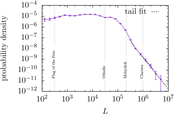
An important characteristic of each text is its length, L, counting the number of word tokens contained in the text. It turns out to be that in the database L expands from very small values up to 4 659 068 tokens, with a distribution that is shown in Fig 1. Observe the roughly uniform distribution up to about L = 10⁵, and the decay afterwards.

Fig 1. Estimation of the probability density function of text length L in the English Project Gutenberg database, using logarithmic binning (5 bins per decade).

Texts with less than 100 tokens are not considered. A power-law fit of the tail [34] yields an exponent 2.92 ± 0.15.

For our analysis we consider only the 31 075 English texts that consist of more than 100 word tokens, as smaller texts would not have statistical value. For each of these texts we select then actual word types (punctuation signs, numbers and any character different from letters are not considered) to count their frequencies n, which will be our primary object of study. The values of these frequencies, for each text, are available on http://dx.doi.org/10.6084/m9.figshare.1515919, in order to facilitate the reproducibility of our results.

In summary, we apply the above described fitting and goodness-of-fit procedure –using ML estimation and the Kolmogorov-Smirnov test– to a total of 31 075 texts from the English Project Gutenberg database, using three different possibilities for the distribution of frequencies: f₁ (Eq (3)), f₂ (Eq (4)), and f₃ (Eq (5)). This yields a total of 3 × 31075 fits and associated p-values, which we analyze and interpret in what follows.

Results

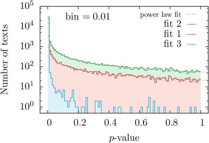
Contrary to previous studies where the number of texts considered was, at most, in the order of tens, the large-scale approach taken in this work requires a statistical analysis of the fitting results, as a case-by-case interpretation is out of hand. We first focus on the distribution of p-values, see Figs 2 and 3. If all texts were truly generated by a mechanism following a given distribution, the corresponding p-values for that distribution would be uniformly distributed between zero and one [56] (see p. 28), [57] (see p.441). As seen in Fig 2, this is not the case and, furthermore, most texts have rather small p-values for the three fits; nevertheless, for distributions f₁ and f₂ there are still many texts that yield high enough p-values.

Fig 2. Histograms of p-values obtained when the Zipf-like distributions f₁, f₂, and f₃ are fitted to the texts of the English Project Gutenberg.

The histograms just count the number of texts in each bin of width 0.01. Note the poor performance of distribution 3 and the best performance of 2. Power-law approximations to the histograms for f₁ and f₂, with respective exponents 0.74 and 0.78, are shown as a guide to the eye.

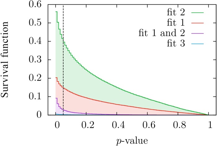
Fig 3. Complementary cumulative distributions (i.e., survival functions) of p-values obtained when our three distributions are fitted to the texts of the English Project Gutenberg.

This corresponds, except for normalization, to the integral of the previous figure, but we have included a fourth curve for the fraction of texts whose p-values for fits 1 and 2 are both higher than the value marked in the abscissa. Note that the values of p can play the role of the significance level. The value for p = 0 is not shown, in order to have higher resolution.

This implies that, although we cannot conclude that the whole database is generated by any of these distributions, these cannot be rejected as good descriptions for large subsets of the database. Regarding distribution f₃, it is clear from the histogram of p-values that it can be discarded as a good description of the distribution of frequencies in any non-negligible subset of texts. So, from now on, we will concentrate on the remaining options, f₁ and f₂, to eventually quantify which of these better describes our corpus. In essence, what we are interested in is which version of Zipf’s law, either distribution f₁ or f₂, fits better a reasonable number of texts, and which range of validity these simple one-parameter distributions have.

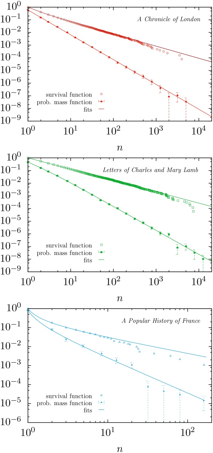
The outcome is that, independently of the significance level (as long as this is not below our resolution of 0.01 given by the number of Monte Carlo simulations), the ratio between the number of texts fitted by distribution f₂ and those fitted by f₁ is nearly constant, taking a value around 2.6. For example, considering significance level (i.e., minimum p-value) equal to 0.05, Fig 3 shows that distribution f₂ fits about 40% of all texts, whereas distribution f₁ fits just 15%. Both percentages include a 2.7% of texts that are fitted by both distributions simultaneously, although this number does not keep a constant ratio with the other two, rather, it decreases when the significance level is increased (as it is implicit in the values of Fig 3). Given that the aforementioned ratio of 2.6 is independent of the significance level, it is fair to say that distribution f₂ provides, compared to f₁, a better description of our database. As a visual illustration of the performance of the fits we display in Fig 4 the word frequency distribution of the longest texts that have p > 1/2, for distributions f₁, f₂ and f₃.

Fig 4. Complementary cumulative distribution and probability mass function of text frequencies, for: (a) A Chronicle of London, from 1089 to 1483 (anonymous); (b) The Works of Charles and Mary Lamb, Vol. V, edited by E. V. Lucas; (c) A Popular History of France from the Earliest Times, Vol. I, by F. Guizot.

These texts are the ones with the largest length L (83 720, 239 018 and 2 081 respectively) of those that fulfill p > 1/2, for fits 1, 2 and 3 respectively. The exponent β takes values 1.96, 1.89, and 1.82, in each case.

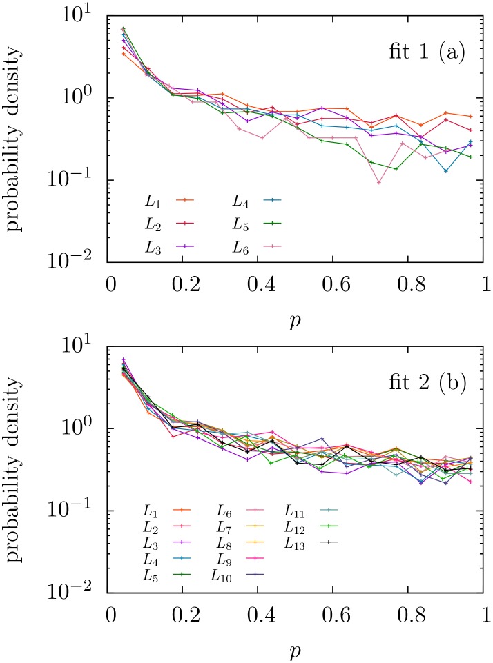
The next question we address is the dependence of the performance of fits on text length L. In order to asses this, note that from the shape of the histograms in Fig 2 we can distinguish two groups of texts: those that lie in the zero bin (whose p-value is strictly less than 0.01), and the rest. Taking the last group, i.e., texts with p ≥ 0.01, and partitioning it into different subsets according to text length (i.e., looking at the distribution of p conditioned to p ≥ 0.01 for different ranges of L), it holds that the shape of the resulting distribution of p does not strongly depend on L, as shown in Fig 5. In contrast, the number of texts that yield p-value near zero certainly varies with L, see Fig 6. Therefore, in order to compare the performances of f₁ and f₂ as a function of the text length L, it is enough to consider a single value of the significance level (greater than zero) as the results for any other significance level will be the same, in relative terms.

Fig 5. Estimated probability density functions of p-values conditioned to p ≥ 0.01 separating for different ranges of text length L. p-values correspond to the fitting of word frequencies to (a) distribution f₁ and (b) distribution f₂.

We divide the distribution of text length into 15 intervals of 2 000 texts each. For distribution f₁ only the first seven groups (up to length 34 400) are displayed (beyond this value we do not have enough statistics to see the distribution of p-values greater than 0.01, as displayed in Fig 6; for distribution 2 this happens only in the last two groups). The intervals L_i range from L₁ = [115, 5291] to L₆ = [25739, 34378] and to L₁₃ = [89476, 103767].

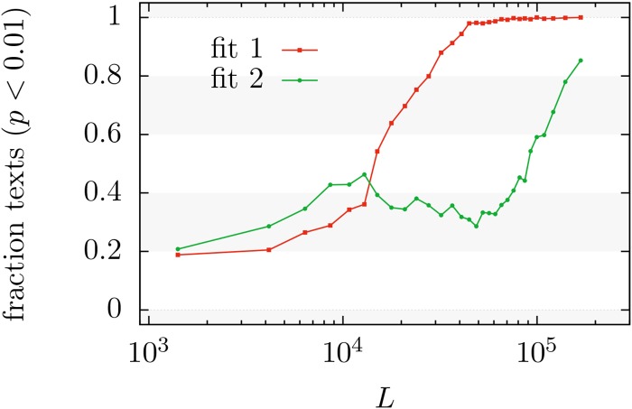
Fig 6. Number of texts with p-value near zero (p < 0.01) in different ranges of L divided by the number of texts in the same ranges, for the fits of distributions f₁ and f₂.

Values of L denote the geometric mean of ranges containing 1000 texts each. The higher value for the fit of f₁ (except for L below about 13000 tokens) denotes its worst performance.

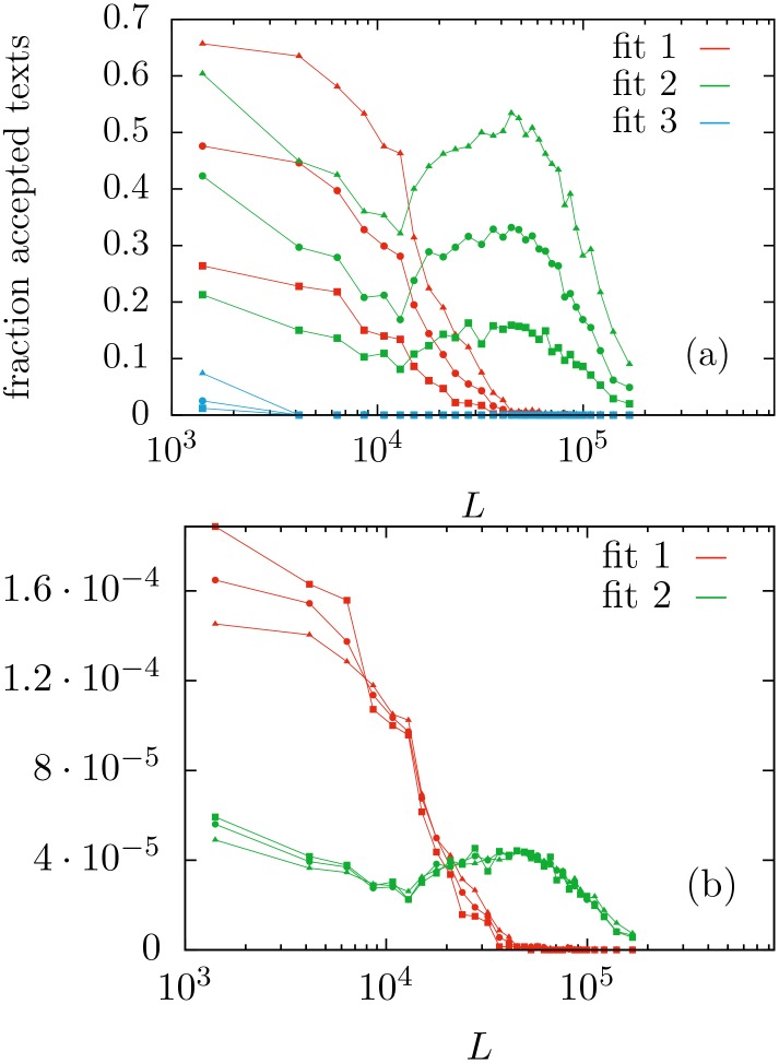
Indeed, Fig 7(a) shows how distribution f₁ fits some more texts than distribution f₂ for small values of L, up to about 13000 tokens. But for larger texts, distribution f₂ clearly outperforms distribution f₁, which becomes irrelevant for L beyond 100000 (at 0.05 significance level), whereas distribution f₂ is able to fit many texts with L larger than 200000. The figure shows that this is the case no matter if the significance level is 0.05, 0.20, or 0.50; the collapse of the curves in Fig 7(b) confirms this fact. From Fig 6 one could infer the same for significance level equal to 0.01. This stability of the performance of the fits for different significance levels arises from the observed fact that the distributions of p-values (conditioned to p ≥ 0.01) are nearly identical for different L, as shown in Fig 5.

Fig 7.

(a) Histograms showing the fraction of accepted texts by the three distributions as a function of their text length, for three different significance levels p₀: 0.05 (upper curves), 0.20 (middle), 0.50 (lower). To be concrete, for each range of L, the ratio between the number of texts with p ≥ p₀ and the number of texts in that range is calculated. (b) Same curves (removing those for distribution 3) under rescaling. We rescale the y—axis by the number of p ≥ p₀, in each case, showing that the relative performance of each fit with regard L is independent on the significance level. Bins are selected to contain 1000 texts each.

Next, we apply the LR test to all texts that have been fitted, considering 0.05 as significance level, by at least one of the two distributions f₁ and f₂. Table 1 merges the results of this test and our previous procedure (based on ML estimation plus the KS test). The total number of texts previously fitted by f₁ or/and f₂ is displayed depending on the sign of the corresponding log-ratio R_1,2. However we must take into account that the sign of the obtained value of R_1,2 could be a product of just statistical fluctuations if the true value were zero and thus, the sign of R_1,2 cannot be trusted in order to discriminate between two models. The probability under the null hypothesis, of obtaining an absolute value of the log-ratio greater than the empirical value |R_1,2| is computed through:

$$p_{LR}=\text{erfc}\left(\frac{|R_{1,2}|}{\sqrt{2N{\sigma }^2}}\right)$$

where erfc is the complementary error function [45]. We will take as statistically significant those R_1,2 that yield p_LR < 0.05. Equivalently, at 0.05 significance level, R_1,2 is significant if its absolute value is greater than $R_c=1.96\sqrt{N{\sigma }^2}$. The results are shown in Table 2

Table 1. Number of texts fitted by f₁, f₂ or both.

	R1,2 > 0	R1,2 < 0	Total ML-KS
f1 (exclusively)	3614	81	3695
f2 (exclusively)	120	11366	11486
f1 and f2	431	398	829
Total LR	4165	11845	16010

The number of texts that are fitted by f₁ or f₂ or both at 0.05 significance level of the ML-KS procedure, separated into two columns according to the sign of R_1,2. Positive R_1,2 means that the likelihood for f₁ is greater than that for f₂, and conversely for negative R_1,2. Nevertheless, the sign of R_1,2 is not an indication of significance, for significant LR tests see Table 2.

Table 2. Number of texts with a significant LR test.

	R1,2 > Rc	R1,2 < −Rc
f1 (exclusively)	1666	0
f2 (exclusively)	0	9423
f1 and f2	0	3
Total LR test	1666	9426
None (neither f1 nor f2)	510	11431

Number of texts with a significant LR test, at the 0.05 level, either favouring distribution f₁ (R_1,2 > R_c) or distribution f₂ (R_1,2 < −R_c), for different outcomes of the ML-KS procedure (at the 0.05 level also). Note that these cases correspond to a subset of the previous table. An additional row shows the number of texts that are fitted neither by distribution f₁ nor f₂; notice that in this case a significant LR test does not guarantee a good fit.

Note that the LR test cannot conclude if a fit is good or bad, as it only compares the relative performance of two fits; in other words, if the LR test selects a particular distribution, that distribution can still yield a bad fit, in absolute terms. Anyway, there is no mismatch between the results of both tests: any time the ML-KS method selects one distribution over the other, the LR test either supports the selection or does not give significant results, but it never selects the other option (as shown in Table 2).

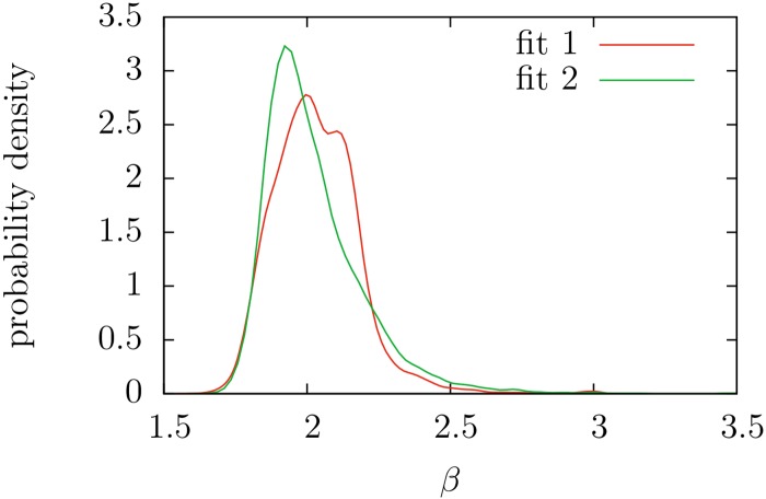
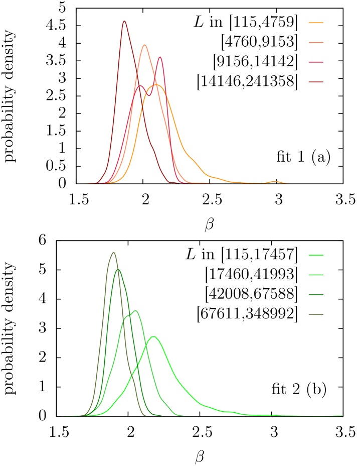
Taking now those texts whose frequency distributions could be approximated by f₁ or f₂, we draw attention to the distribution of the estimated exponents (i.e., the parameter β). The original formulation of Zipf’s law implies β = 2 and Fig 8 shows that β is certainly distributed around 2, with a bell-like shape, and the range of variation is, more or less, between 1.6 and 3. The lower value β ≃ 1.6 is in surprising good agreement with the results of the information-theoretic model of Ref. [58], whereas the upper limit β ≃ 3 is somewhat larger than the results of that model. Moreover, the distributions of β are not symmetric, and the upper limit cannot be defined so sharply as the lower limit. Notice also that texts with limiting values of the exponents do not correspond, in principle, to pathological texts, as claimed in Ref. [58]; rather, for the smallest β we find theatre (including Tosltoy and Ibsen) and children books (some by Jane L. Stewart), whereas the largest β correspond to short poems.

Fig 8. Estimation of the probability density of the Zipf’s exponent β for texts yielding p ≥ 0.05 in the fits of f₁ and f₂.

Curves have been calculated from the histograms via normal kernel smoothing method as implemented in MatLab (ksdensity function). Estimated mean and standard deviation of β are 2.03 and 0.15 respectively for the fit of f₁, and 2.02 and 0.17 for f₂.

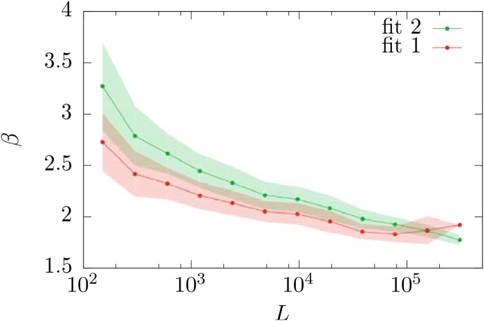
If we check the effect of the text length L in the distribution of β, we find a decreasing trend of β with L, as can be seen in Figs 9 and 10. We have tested that this observation is not an artifact of the fitting method, as synthetic texts generated with fixed β do not show this behavior. This trend is not in disagreement with the claims of Ref. [35], where the stability of the exponent β was demonstrated for a single growing text (i.e., comparing small parts of a text with the whole). A possible explanation for the decrease of β with L could be a systematic dependence of β with genre, and a bias of L with genre. At present we do not have an automatic way to assign genres to texts and we cannot test this hypothesis.

Fig 9. Estimated probability density of β for fits with p ≥ 0.05, in different length ranges.

We have divided both groups of accepted texts into 4 percentiles according to L. As in the previous figure, the normal kernel smoothing method is applied. (a) For distribution f₁. (b) For distribution f₂.

Fig 10. Mean value and standard deviation (represented by the shaded regions) of the distribution of the Zipf’s exponent β as a function of text length L for distributions f₁ and f₂.

Note that the last bin of f₁ contains a single datapoint, and so its standard deviation is not defined.

Discussion and Conclusions

Zipf’s law is probably the most intriguing and at the same time well-studied experimental law of quantitative linguistics, and extremely popular in its wider sense in the science of complex systems. Although the previous literature is vast, as far as we know our work constitutes the first large-scale analysis of Zipf’s law in single (non-aggregated) texts. Thus, we are in a position to make a well-grounded statement about the validity of Zipf’s law in such texts (when those are written in English).

Let us first briefly summarize, however, some key technical points of our study. First, we have analyzed a total of 31 075 English texts from the Project Gutenberg database using rigorous fitting procedures, and have tested how well they are described by three Zipf-like distributions. Our choice of distributions has not been exhaustive; rather, we have limited ourselves to different interpretations of what can be understood as “Zipf’s law”, in the sense of having a perfect power law either in the probability mass function of word frequencies, or in the complementary cumulative distribution function (whose empirical estimation leads to the rank-frequency relation of the sample), or in the rank-frequency relation of an underlying population. Remarkably, the resulting distributions have a unique parameter, β, which in all cases is the exponent of an asymptotic power law in the probability mass function of the frequency. It is left to explore how other, more complicated extensions of Zipf’s law perform on this large corpus, but it is obvious that, by including additional parameters, one might provide good fits to a larger number of texts (although in this case, proper model selection will require to balance number of parameters and parsimony).

Our aim in this paper has not been to fit as many texts as possible, but to test the performance of the simplest Zipf-like distributions within a very strict, conservative framework. Indeed, by requiring the three versions of Zipf’s law to hold on the full range of frequencies n = 1, 2, … (and not only on the tail of the distribution) we put ourselves in the strictest range of demands. It is hence remarkable that, e.g., at the standard significance level of 0.05, and for text lengths between 10⁴ and 10⁵ word tokens, more than 40% of the considered texts are statistically compatible with the pure power law in the complementary cumulative distribution function represented by distribution f₂ (see Fig 7). So, we can state that, for the corpus under consideration, the most appropriate version of Zipf’s law is given by a probability mass function

$$f\left(n\right)=\text{Prob}[\text{frequency}=n]=\frac{1}{n^{\beta -1}}-\frac{1}{{(n+1)}^{\beta -1}},$$

or, equivalently, by a complementary cumulative distribution function

$$S\left(n\right)=\text{Prob}[\text{frequency}\ge n]=\frac{1}{n^{\beta -1}}.$$

Due to the broad coverage of the Project Gutenberg corpus we speculate that this distribution should fit a large fraction of generic (non-technical) English texts. Of course, testing this speculation in front of all possible corpora is an impossible task.

We have also shown that our conclusions regarding the relative performance of a pure power law in the probability mass function, given by distribution f₁, versus distribution f₂ are robust with respect to changes in the significance level: about twice as many texts are statistically compatible with distribution f₂ than those compatible with f₁, at any significance level (obviously, in absolute terms, the number of accepted texts varies with the significance level). Hence we can conclude that distribution f₂ gives a better description of English texts than distribution f₁, at least for the corpus considered in this work.

We may speculate that the predominance of f₂ in front of f₁ (and in front of f₃) may be a peculiarity of the English language, caused by its poor inflectional morphology. Indeed, the difference between these distributions is in the lowest frequencies (mainly n = 1, n = 2…). Languages with a richer inflectional morphology should yield a larger proportion of low-frequency words (in comparison to the other words) than English, favoring perhaps f₁ in front of f₂. This analysis is left for future studies. Lemmatization of texts [6] would be very helpful to test this speculation, but at present we cannot afford large-scale lemmatization.

Another conclusion is that distribution f₃, first derived by Mandelbrot [40], is irrelevant for the description of texts in this corpus. Finally, we have corroborated that the exponent β of Zipf’s law certainly varies from text to text, as had been previously claimed using other approaches for defining what Zipf’s law is [5, 6]. Interestingly, the value β = 2 originally proposed by Zipf himself is among the most frequent ones.

We believe that our analysis constitutes a major advancement in the understanding of Zipf’s law. It is astonishing how good the simplest one-parameter Zipf-like distributions perform on such a large set of texts, particularly with the strict set of requirements we have imposed. This is in sharp contrast for instance with Zipf’s law in demography [59] and in the distribution of income [60], where the power law seems to be valid only for the tail corresponding to the largest sizes, as it happens also for the distribution of word frequency in large text corpora, as mentioned above [2, 36–39].

Zipf’s law has been subject to much debate, and will probably continue to be so for many years. Indeed, one can always cast doubt on its validity on the basis of some particular examples. Yet it seems clear to us that, in our modern times of big data and large computational capabilities, more efforts should be put towards large-scale analysis of Zipf’s law. We hope this paper constitutes a first step in this direction.

Appendix: Simulation of Discrete Zipf-like Distributions

As part of the testing procedure, we need simulated samples from f₁, f₂, and f₃, which are discrete distributions defined for n = a, a + 1, …. We will give the recipe of simulation for an arbitrary positive integer value of the lower cut-off a. It is simpler to start with f₂, as this is used as an auxiliary distribution in the simulation of the other two.

Simulation of f₂

Fixed a and given the parameter β, we want a set of random numbers whose complementary cumulative distribution function is a discrete power law: S₂(n) = (a/n)^β−1. For that, we first generate a random number u from a uniform distribution in the interval (0, u_max), with u_max = 1/a^β−1. The inversion method [56, 57] guarantees that if we take x = 1/u^1/(β−1), the values of x yield a continuous power law with $S_2^c\left(x\right)={\left(a/x\right)}^{\beta -1}$, for x ≥ a, where the superscript c distinguishes the continuous distribution from its discrete analogous one. So, taking n equal to the integer part of x, i.e., n = int(x), yields a discrete distribution with S₂(n) = (a/n)^β−1, as desired. This is so because, for any X, int(X) ≥ n is equivalent to X ≥ n for n integer. In a recipe:

1. generate u from a uniform distribution in (0, 1/a^β−1],

2. calculate x = 1/u^1/(β−1),

3. take n = int(x).

By means of the so-called rejection method [56, 57], simulated integers distributed following f₂ can be used for the simulation of integers following f₁ or f₃. The key point to achieve a high performance in the rejection method is to use a “good” auxiliary function, i.e., one that leads to a low rejection rate. This is certainly the case in our framework, as explained below.

Simulation of f₁

In this case, the steps are:

1. generate n from f₂(n),

2. generate v from a uniform distribution in the unit interval,

3. n is accepted if

   $$v\le \frac{f_1\left(n\right)}{f_2\left(n\right)C},$$

   and rejected otherwise, where C is the rejection constant given by C = max_{n ≥ a}{f₁(n)/f₂(n)}.

Note that the rejection method [56, 57] guarantees that the resulting (non-rejected) n will be distributed according to f₁.

It is easy to check that the maximum of f₁/f₂ is reached at n = a as this is a decreasing function [41]. The acceptance condition above can be simplified by taking τ = (1 + n⁻¹)^β−1, and b = (1 + a⁻¹)^β−1, then, the condition becomes:

$$bvn(\tau -1)\le a(b-1)\tau ,$$

which is devoid of the calculation of the Hurwitz-zeta function. This is a generalization for a > 1 of the method of Ref. [56]. The choice of f₂ as the auxiliary distribution function is justified by the small value that C takes, as this is the expected number of generated values of n until we accept one. For instance, for β = 2 and a = 1 we get C = 1.2158.

Simulation of f₃

Proceeding similarly, we get in this case low values of C = max_{n ≥ a}{f₃(n)/f₂(n)} as well (we get C = 2 in the limit β → 2 for a = 1). The maximum of f₃(n)/f₂(n) is numerically seen to be reached at n = a. In summary, the steps are:

1. generate n from f₂(n)

2. generate v from a uniform distribution in the unit interval

3. n is accepted if

   $$v{f}_2\left(n\right)\le a\left(1-{\left(\frac{a}{a+1}\right)}^{\beta -1}\right)\frac{\Gamma (n-(\beta -1\left)\right)}{\Gamma (n+1)}\frac{\Gamma \left(a\right)}{\Gamma (1+a-\beta )}$$

   and rejected otherwise.

Data Availability

All word-count files are available at http://dx.doi.org/10.6084/m9.figshare.1515919.

Funding Statement

This work was supported by Ministerio de Economia y Competitividad (Gobierno de España) (http://www.mineco.gob.es/), grant number FIS2012-31324 (receiver: ACC) and Agència de Gestió d’Ajust Universitaris i de Recerca (Generalitat de Catalunya) (http://www10.gencat.cat/agaur_web/AppJava/catala/index.jsp), grant number 2014SGR-1307 (receiver: ACC). The funders had no role in study design, data collection and analysis, decision to publish, or preparation of the manuscript.

References

- 1. Baayen H. Word Frequency Distributions. Kluwer, Dordrecht; 2001. [Google Scholar]
- 2. Baroni M. Distributions in Text In: Lüdeling A, Kytö M, editors. Corpus linguistics: An international handbook, Volume 2 Mouton de Gruyter, Berlin; 2009. p. 803–821. [Google Scholar]
- 3.Zanette D. Statistical Patterns in Written Language. arXiv. 2014;1412.3336v1.
- 4. Piantadosi ST. Zipf’s law in natural language: a critical review and future directions. Psychon Bull Rev. 2014;21:1112–1130. Available from: http://colala.bcs.rochester.edu/papers/piantadosi2014zipfs.pdf. 10.3758/s13423-014-0585-6 [DOI] [PMC free article] [PubMed] [Google Scholar]
- 5. Zanette D, Montemurro M. Dynamics of Text Generation with Realistic Zipf’s Distribution. J Quant Linguist. 2005;12(1):29–40. 10.1080/09296170500055293 [DOI] [Google Scholar]
- 6. Corral A, Boleda G, Ferrer-i-Cancho R. Zipf’s Law for Word Frequencies: Word Forms versus Lemmas in Long Texts. PLoS ONE. 2015;10(7):e0129031 10.1371/journal.pone.0129031 [DOI] [PMC free article] [PubMed] [Google Scholar]
- 7. Bentz C, Verkerk A, Kiela D, Hill F, Buttery P. Adaptive Communication: Languages with More Non-Native Speakers Tend to Have Fewer Word Forms. PLoS ONE. 2015;10(6):e0128254 10.1371/journal.pone.0128254 [DOI] [PMC free article] [PubMed] [Google Scholar]
- 8. Serrà J, Corral A, Boguñá M, Haro M, Arcos JL. Measuring the Evolution of Contemporary Western Popular Music. Sci Rep. 2012;2:521 10.1038/srep00521 [DOI] [PMC free article] [PubMed] [Google Scholar]
- 9. Haro M, Serrà J, Herrera P, Corral A. Zipf’s Law in Short-Time Timbral Codings of Speech, Music, and Environmental Sound Signals. PLoS ONE. 2012;7:e33993 10.1371/journal.pone.0033993 [DOI] [PMC free article] [PubMed] [Google Scholar]
- 10. Li W. Zipf’s law everywhere. Glottom. 2002;5:14–21. [Google Scholar]
- 11. Axtell RL. Zipf Distribution of U.S. Firm Sizes. Science. 2001;293:1818–1820. 10.1126/science.1062081 [DOI] [PubMed] [Google Scholar]
- 12. Clauset A, Shalizi CR, Newman MEJ. Power-law distributions in empirical data. SIAM Rev. 2009;51:661–703. 10.1137/070710111 [DOI] [Google Scholar]
- 13. Pueyo S, Jovani R. Comment on “A Keystone Mutualism Drives Pattern in a Power Function”. Science. 2006;313:1739c–1740c. [DOI] [PubMed] [Google Scholar]
- 14. Camacho J, Solé RV. Scaling in ecological size spectra. Europhys Lett. 2001;55:774–780. 10.1209/epl/i2001-00347-0 [DOI] [Google Scholar]
- 15. Adamic LA, Huberman BA. Zipf’s law and the Internet. Glottometrics. 2002;3:143–150. [Google Scholar]
- 16. Newman MEJ. Power laws, Pareto distributions and Zipf’s law. Cont Phys. 2005;46:323–351. 10.1080/00107510500052444 [DOI] [Google Scholar]
- 17. Furusawa C, Kaneko K. Zipf’s law in gene expression. Phys Rev Lett. 2003;90:088102 10.1103/PhysRevLett.90.088102 [DOI] [PubMed] [Google Scholar]
- 18. Simon HA. On a Class of Skew Distribution Functions. Biomet. 1955;42:425–440. 10.2307/2333389 [DOI] [Google Scholar]
- 19. Miller GA. Some Effects of Intermittent Silence. Am J Psychol. 1957;70(2):311–314. 10.2307/1419346 [DOI] [PubMed] [Google Scholar]
- 20. Ferrer i Cancho R, Solé RV. Least effort and the origins of scaling in human language. Proc Natl Acad Sci USA. 2003;100:788–791. 10.1073/pnas.0335980100 [DOI] [PMC free article] [PubMed] [Google Scholar]
- 21. Mitzenmacher M. A Brief History of Generative Models for Power Law and Lognormal Distributions. Internet Math. 2004;1 (2):226–251. 10.1080/15427951.2004.10129088 [DOI] [Google Scholar]
- 22. Saichev A, Malevergne Y, Sornette D. Theory of Zipf’s Law and of General Power Law Distributions with Gibrat’s Law of Proportional Growth Lecture Notes in Economics and Mathematical Systems. Springer Verlag, Berlin; 2009. [Google Scholar]
- 23. Corominas-Murtra B, Fortuny J, Solé RV. Emergence of Zipf’s Law in the Evolution of Communication. Phys Rev E. 2011;83:036115. 10.1103/PhysRevE.83.036115 [DOI] [PubMed] [Google Scholar]
- 24. Peterson J, Dixit PD, Dill KA. A maximum entropy framework for nonexponential distributions. Proc Natl Acad Sci USA. 2013;110(51):20380–20385. Available from: http://www.pnas.org/content/110/51/20380.abstract. 10.1073/pnas.1320578110 [DOI] [PMC free article] [PubMed] [Google Scholar]
- 25. Corominas-Murtra B, Hanel R, Thurner S. Understanding scaling through history-dependent processes with collapsing sample space. Proc Natl Acad Sci USA. 2015;112(17):5348–5353. Available from: http://www.pnas.org/content/112/17/5348.abstract. 10.1073/pnas.1420946112 [DOI] [PMC free article] [PubMed] [Google Scholar]
- 26. Ferrer-i-Cancho R, Elvevåg B. Random Texts Do Not Exhibit the Real Zipf’s Law-Like Rank Distribution. PloS One. 2010;5(3):e9411 10.1371/journal.pone.0009411 [DOI] [PMC free article] [PubMed] [Google Scholar]
- 27. Prokopenko M, Ay N, Obst O, Polani D. Phase transitions in least-effort communications. J Stat Mech. 2010;2010(11):P11025 Available from: http://stacks.iop.org/1742-5468/2010/i=11/a=P11025. 10.1088/1742-5468/2010/11/P11025 [DOI] [Google Scholar]
- 28. Dickman R, Moloney NR, Altmann EG. Analysis of an information-theoretic model for communication. J Stat Mech: Theory Exp. 2012;P12022. 10.1088/1742-5468/2012/12/P12022 [DOI] [Google Scholar]
- 29. Li W, Miramontes P, Cocho G. Fitting ranked linguistic data with two-parameter functions. Entropy. 2010;12(7):1743–1764. 10.3390/e12071743 [DOI] [Google Scholar]
- 30. Goldstein ML, Morris SA, Yen GG. Problems with fitting to the power-law distribution. Eur Phys J B. 2004;41:255–258. 10.1140/epjb/e2004-00316-5 [DOI] [Google Scholar]
- 31. Bauke H. Parameter estimation for power-law distributions by maximum likelihood methods. Eur Phys J B. 2007;58:167–173. 10.1140/epjb/e2007-00219-y [DOI] [Google Scholar]
- 32. White EP, Enquist BJ, Green JL. On estimating the exponent of power-law frequency distributions. Ecol. 2008;89:905–912. 10.1890/07-1288.1 [DOI] [PubMed] [Google Scholar]
- 33. Casella G, Berger RL. Statistical Inference. 2nd ed Duxbury, Pacific Grove CA; 2002. [Google Scholar]
- 34. Deluca A, Corral A. Fitting and goodness-of-fit test of non-truncated and truncated power-law distributions. Acta Geophys. 2013;61:1351–1394. 10.2478/s11600-013-0154-9 [DOI] [Google Scholar]
- 35. Font-Clos F, Boleda G, Corral A. A scaling law beyond Zipf’s law and its relation with Heaps’ law. New J Phys. 2013;15:093033. 10.1088/1367-2630/15/9/093033 [DOI] [Google Scholar]
- 36. Ferrer i Cancho R, Solé RV. Two regimes in the frequency of words and the origin of complex lexicons: Zipf’s law revisited. J Quant Linguist. 2001;8(3):165–173. 10.1076/jqul.8.3.165.4101 [DOI] [Google Scholar]
- 37. Petersen AM, Tenenbaum JN, Havlin S, Stanley HE, Perc M. Languages cool as they expand: Allometric scaling and the decreasing need for new words. Sci Rep. 2012;2:943 10.1038/srep00943 [DOI] [PMC free article] [PubMed] [Google Scholar]
- 38. Gerlach M, Altmann EG. Stochastic model for the vocabulary growth in natural languages. Phys Rev X. 2013;3:021006. [Google Scholar]
- 39.Williams JR, Bagrow JP, Danforth CM, Dodds PS. Text mixing shapes the anatomy of rank-frequency distributions: A modern Zipfian mechanics for natural language. arXiv. 2015;1409.3870v3. [DOI] [PubMed]
- 40. Mandelbrot B. On the theory of word frequencies and on related Markovian models of discourse In: Jakobson R, editor. Structure of Language and its Mathematical Aspects. Providence, RI: American Mathematical Society; 1961. p. 190–219. [Google Scholar]
- 41.Corral A, i Cancho RF. (in preparation). 2015;.
- 42. Kolmogorov AN. Foundations of the theory of probability. 2nd ed Chelsea Pub. Co., New York; 1956. [Google Scholar]
- 43.Altmann EG, Gerlach M. Statistical laws in linguistics. arXiv. 2015;1502.03296.
- 44. Font-Clos F, Corral A. Log-Log Convexity of Type-Token Growth in Zipf’s Systems. Phys Rev Lett. 2015;114:238701. 10.1103/PhysRevLett.114.238701 [DOI] [PubMed] [Google Scholar]
- 45. Abramowitz M, Stegun IA, editors. Handbook of Mathematical Functions. Dover, New York; 1965. [Google Scholar]
- 46. Pawitan Y. In All Likelihood: Statistical Modelling and Inference Using Likelihood. Oxford UP, Oxford; 2001. Available from: http://books.google.es/books?id=njqJxqKk2GAC. [Google Scholar]
- 47. Press WH, Teukolsky SA, Vetterling WT, Flannery BP. Numerical Recipes in C. 2nd ed Cambridge University Press, Cambridge; 1992. [Google Scholar]
- 48. Corral A, Font F, Camacho J. Non-characteristic Half-lives in Radioactive Decay. Phys Rev E. 2011;83:066103 10.1103/PhysRevE.83.066103 [DOI] [PubMed] [Google Scholar]
- 49. Corral A, Deluca A, Ferrer-i-Cancho R. A practical recipe to fit discrete power-law distributions. ArXiv. 2012;1209:1270. [Google Scholar]
- 50. Abdi H. Bonferroni and Šidák corrections for multiple comparisons In: Salkind NJ, editor. Encyclopedia of Measurement and Statistics. Sage, Thousand Oaks; 2007. p. 103–107. [Google Scholar]
- 51. Bland JM, Altman DG. Multiple significance tests: the Bonferroni method. Brit Med J. 1995;310:170–170. 10.1136/bmj.310.6973.170 [DOI] [PMC free article] [PubMed] [Google Scholar]
- 52. Benjamini Y, Hochberg Y. Controlling the False Discovery Rate: A Practical and Powerful Approach to Multiple Testing. J Roy Stat Roc B. 1995;57:289–300. [Google Scholar]
- 53. Vuong QH. Likelihood Ratio Tests for Model Selection and Non-nested Hypotheses. Econometrica. 1989;57(2):307–33. Available from: http://EconPapers.repec.org/RePEc:ecm:emetrp:v:57:y:1989:i:2:p:307-33. 10.2307/1912557 [DOI] [Google Scholar]
- 54.Project Gutenberg;http://www.gutenberg.org.
- 55.Wikipedia (accessed August 2015);https://en.wikipedia.org/wiki/Project_Gutenberg.
- 56. Devroye L. Non-Uniform Random Variate Generation. Springer-Verlag, New York; 1986. [Google Scholar]
- 57. Ross SM. A First Course in Probability. 8th ed Prentice Hall, Englewood Cliffs; 2010. [Google Scholar]
- 58. Ferrer i Cancho R. The variation of Zipf’s law in human language. Eur Phys J B. 2005;44(2):249–257. 10.1140/epjb/e2005-00121-8 [DOI] [Google Scholar]
- 59. Malevergne Y, Pisarenko V, Sornette D. Testing the Pareto against the lognormal distributions with the uniformly most powerful unbiased test applied to the distribution of cities. Phys Rev E. 2011;83:036111 10.1103/PhysRevE.83.036111 [DOI] [PubMed] [Google Scholar]
- 60. Drăgulescu A, Yakovenko VM. Exponential and power-law probability distributions of wealth and income in the United Kingdom and the United States. Physica A. 2001;299(1–2):213–221. Available from: 10.1016/S0378-4371(01)00298-9. 10.1016/S0378-4371(01)00298-9 [DOI] [Google Scholar]
Associated Data
This section collects any data citations, data availability statements, or supplementary materials included in this article.
Data Availability Statement