Quantitative analysis of ultrasound images for computer-aided diagnosis

Abstract.

We propose an adaptable framework for analyzing ultrasound (US) images quantitatively to provide computer-aided diagnosis using machine learning. Our preliminary clinical targets are hepatic steatosis, adenomyosis, and craniosynostosis. For steatosis and adenomyosis, we collected US studies from 288 and 88 patients, respectively, as well as their biopsy or magnetic resonanceconfirmed diagnosis. Radiologists identified a region of interest (ROI) on each image. We filtered the US images for various texture responses and use the pixel intensity distribution within each ROI as feature parameterizations. Our craniosynostosis dataset consisted of 22 CT-confirmed cases and 22 age-matched controls. One physician manually measured the vectors from the center of the skull to the outer cortex at every 10 deg for each image and we used the principal directions as shape features for parameterization. These parameters and the known diagnosis were used to train classifiers. Testing with cross-validation, we obtained 72.74% accuracy and 0.71 area under receiver operating characteristics curve for steatosis ($p<0.0001$), 77.27% and 0.77 for adenomyosis ($p<0.0001$), and 88.63% and 0.89 for craniosynostosis ($p=0.0006$). Our framework is able to detect a variety of diseases with high accuracy. We hope to include it as a routinely available support system in the clinic.

1. Introduction

This work presents an adaptable ultrasound (US) computer-aided diagnosis framework that is suitable for clinical application across physicians, disease types, devices, and operators. US is one of the most widely utilized imaging modalities because it is quick, safe, easy to use, and inexpensive compared to other modalities. However, US is limited by its high-operator dependence, inter-reader variability, and dependence on machine settings.¹ Computer-aided diagnosis can improve confidence in US through quantitative analysis. In particular, we looked at abnormalities in texture in hepatic steatosis and adenomyosis, and shape in craniosynostosis. Our clinical aims are to provide a straightforward framework for developing a library of tools specific to various image assessment tasks that can increase confidence in diagnosis, and increase detection rates to provide earlier intervention.

2. Related Work

2.1. Texture Analysis for Steatosis Detection

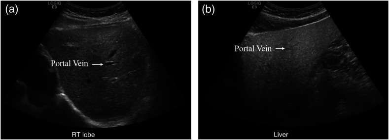
We initially looked at the clinical targets of diagnosing hepatic steatosis, adenomyosis, and craniosynostosis from US images. Steatosis is abnormal lipid retention. In particular, we focused on steatosis in the liver, which has prevalence of $\sim 31\%$ in the general population.² While early damage is reversible, long-term steatosis can lead to more severe liver conditions such as cirrhosis and liver failure.³ US is the initial modality to examine patients with suspected steatosis.⁴ The differences between healthy and abnormal tissue are very subtle, as shown in Fig. 1. Frequently, doctors are not confident and need to confirm their diagnosis with biopsy.⁵ This more invasive procedure delays intervention and increases the risk for the patient.

Fig. 1.

US of (a) normal versus (b) fatty liver. The texture of the right image is in general grainier, but some speckling, inherently caused by the US medium, can be seen on the left image as well. The portal vein shows up more clearly in the left image as fatty liver obscures the vessel interface. Additionally, fatty liver is more hyperechoic. Compared to the evenly bright normal liver, the top of the right US image (near the surface) is much brighter than the bottom (deeper) as more sound waves are immediately reflected in the fatty liver.

Previous works have examined the pattern of echogenic pixels of US images, referred to as US texture, as a noninvasive, quantitative method to diagnose steatosis. Texture characteristics derive from a combination of changes to the underlying tissue and the noise the imaging modality introduces.⁶ In the case of US, shadowing and speckling introduce error to the true texture of the image.

Specifically, texture changes in the liver due to steatosis have been well studied. Clinical observations include that livers turn from smooth and dark to coarse and grainy as their fat content increases. Some time ago, Khoo et al.⁷ established that steatosis can be detected using US imaging due to the relatively higher echogenicity of fatty tissue. The method proposed by Khoo is based on frequency response. While the trend in the energy is noticeable, there was no clear boundary between none/mild/moderate cases. Similarly, Lee et al.⁸ measured the effectiveness of standard deviation of pixel intensity to classify US liver images as normal/fatty liver/chronic liver disease. Their study includes 202 patients and demonstrates that the mean value of the standard deviation is significantly higher in patients with chronic liver disease. However, the ranges of the three categories overlap too much to confidently diagnose patients using only the standard deviation.

These studies show promising preliminary results, but they are mostly limited in size and diversity of the image collection settings. The individual features studied do not provide robust enough separation to use in a clinical setting. The problem of creating a dependable framework to systematically quantify US images is still an open problem. Our method aims to combine many features and use machine learning to identify the most relevant ones, and show that these features can provide reliable differentiation in a larger patient group collected from a retrospective review of images. We draw upon previously identified relevant texture features and combine them to increase confidence in our classifications. Starting with a broad range of previously identified features, we use cross-validation on a high-performance computing cluster to narrow down which are the most relevant.

2.2. Texture Analysis for Adenomyosis Detection

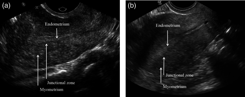
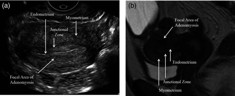
The uterus is composed of two distinct tissue layers, the thinner hormonally stimulated endometrium and the relatively static myometrium. Adenomyosis is defined as ectopic endometrial tissue within the myometrium. Clinical data reports anywhere from 5% to 70% prevalence in women.⁹ Diagnosis sensitivity and specificity range from 53% to 89% and 50% to 99%, respectively, for transvaginal US¹⁰ and Bazot et al.¹¹ report 32.5% sensitivity and 95% specificity in transabdominal US. Classic US imaging findings of adenomyosis include a globular shape to the uterus and subendometrial linear striations and cystic spaces. Figure 2 shows a comparison of a healthy pelvic US to one with adenomyosis. While MRI remains the imaging gold standard for diagnosis, the first line imaging modality for the nonspecific symptoms with which these patients typically present—heavy menstrual bleeding, cramps, and cyclical pelvic pain—is often pelvic US. It is less expensive and more readily available. The symptoms may be dismissed as normal menstrual symptoms and not considered urgent enough to be scheduled for this more expensive test. It is also associated with infertility.¹²

Fig. 2.

Pelvic US of a patient (a) with adenomyosis and (b) one without. The regions of the uterus are not well distinguished from each other, and it is difficult to see changes caused by the adenomyosis.

Hysterectomy is the accepted treatment, but newer techniques such as uterine artery embolization show promise.⁹ An earlier and more confident diagnosis through US would provide better treatment planning for patients to control associated symptoms. Kepkep et al.¹³ found that textural features such as subendometrial linear striation and heterogeneous myometrium are indicative of the disease. Hypothesizing that these texture changes can be detected by a computer, we apply to uterine US the same texture detection framework used for steatosis.

2.3. Shape Analysis for Craniosynostosis Detection

Craniosynostosis is the premature fusing of sutures in an infant’s head, affecting about $1/2000$ births.¹⁴ As the infant’s brain is expanding, the fusion causes increased intracranial pressure and could affect brain development.¹⁵ For craniosynostosis involving only one suture, intervention within the first year of life generally leads to a good prognosis, but the ideal timing for intervention varies from 6 weeks to 10 months by which sutures are affected.^16,17 It is currently only diagnosed postnatally, typically through physical examination. As physical examination is sometimes uncertain immediately after birth, this can cause delayed diagnosis or a need for computed tomography to confirm, which raises radiation concerns.¹⁷

Previous work had focused on prenatally identifying craniosynostosis in a high-risk population and focused on more severe, syndromic forms of the disease.¹⁸ The same method led to high-false positives in the general population.^14,18 They also relied on expert readers to read the images.

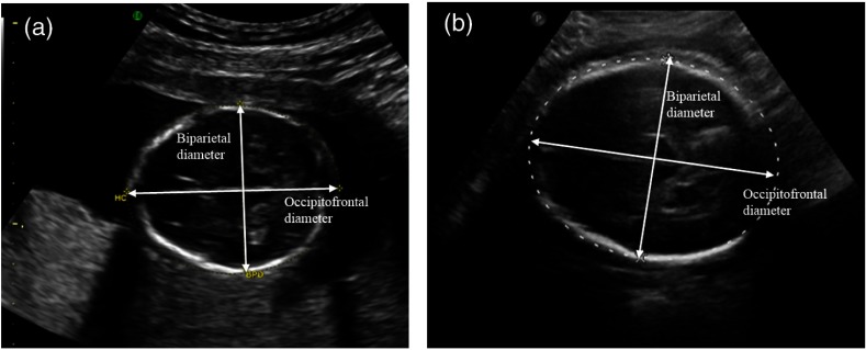
Prenatal US presents the challenge of tracing three-dimensional sutures using two-dimensional (2-D) US.¹⁸ Figure 3 shows an example of a 2-D projection of a skull with craniosynostosis compared to one without. Since the time and type of intervention varies from case to case,¹⁷ the earlier detection will help doctors better monitor skull development and plan treatment, as well as counsel parents.

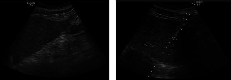
Fig. 3.

US of a fetus (a) who will develop craniosynostosis and (b) one who will not. By manual inspection, the difference between the two is not obvious at this stage. This is further complicated by the imaging medium, where the front and back of the skull are sometimes indistinct, as shown in the right image.

Delahaye et al.¹⁴ found that brachycephaly and dolichocephaly, shorter and longer head shape than the expected range, are not good predictors of craniosynostosis by themselves. These features are only indicative of craniosynostosis when combined with associated syndromes or fetal DNA abnormalities. In the general population, they found very high levels of false positives. Our study uses additional shape information and analysis to improve accuracy in the general population, and use a machine learning framework to reduce reliance on expert readers.

2.4. Machine Learning

We use machine-learning algorithms to train classifiers and label images as normal versus abnormal based on the identified features of the images. In particular, we use support vector machines (SVM)¹⁹ and random forest (RF).²⁰ In an SVM, the parameterization of each image is plotted in high-dimensional spaces, and the algorithm finds the best hyperplane to separate the abnormal training data from the normal. The RF algorithm, on the other hand, separates the normal and abnormal parameters by decision trees. It has a number of subclassifiers, called trees, and each one classifies the image as sick or not sick based on a subset of the parameters. To classify a new image, each tree classifies it based on its subset of parameters, and the overall majority classification determines the result.

Although the machine-learning algorithm presents a more objective evaluation than a human reader, inter-reader variability still poses challenges. Vicas et al.¹ show that if the training and test region of interest (ROI) are both identified by the same reader, machine-learning algorithms generally do better than if each were determined by a different reader. They propose an algorithm to automatically identify a suitable texture ROI in liver US imaging following the constraint to avoid structural elements like blood vessels and bile ducts. However, this automatic method sometimes fails to identify any ROI under those constraints, even when human readers do find ROIs in the same image.

Minhas et al.⁴ present a completely automated system to classify liver US images for fatty liver disease by automatically identifying a ROI. They achieved sensitivities, specificities, and accuracies above 90%. Their images were homogeneous with respect to machine and machine settings, and class labels for their training and testing sets came from human readers rather than liver biopsies. Since results are reader dependent,¹ this bias results in favor of the algorithm. Li et al.²¹ obtained over 84% accuracy in classifying fatty and normal liver by looking at near- and far-field ROIs and measuring the light density and neighborhood gray scale characteristics. Their data set was heterogeneous with respect to operator and anatomic view, but the study restricted US machine setting such as frequency, gain, and depth.

In contrast to the previous work, the framework described here can be trained from populations of extant clinical images, tuned for sensitivity and specificity, and used prospectively for quantitative clinical decision-making support. It can be extended to include additional parameters. Alternate machine-learning paradigms can also be easily integrated and evaluated.

3. Models and Methods

3.1. Data Collection

All scans were obtained using GE LOGIQ E9 US units. We did not control for probe type.

3.1.1. Steatosis

For the steatosis study, we collected data from Rhode Island Hospital (RIH) from 354 patients with random US-guided liver biopsies between 2009 and 2013. This retrospective study was heterogeneous with regard to device settings, operator characteristics, and anatomic view. From these patients, we collected 624 liver US images and the patient’s corresponding quantitative values of fat (%) from pathology. Patients with targeted biopsies were excluded, since tumors affect fat content. After removing patients with targeted biopsies, we had 488 images from 288 patients. This data review was approved by RIH Institutional Review Board (IRB) as study 007313 on March 23, 2013.

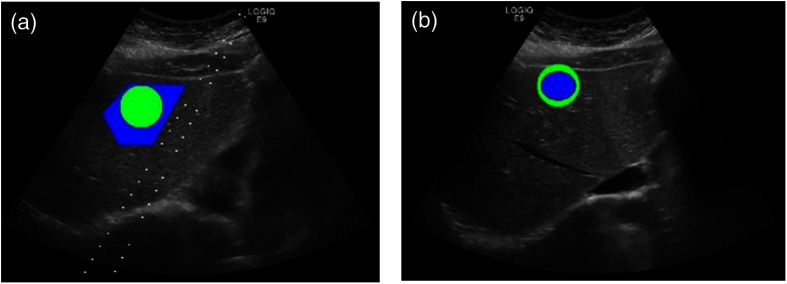
Two experienced radiologists independently examined all of the images in the steatosis dataset. They were blinded to the biopsy results. Each radiologist chose an image in each patient’s series of images that best displayed the hepatic echo-texture. On that image, each drew an ROI using ImageJ,²² as shown in Fig. 4. They were not looking specifically for steatosis or its absence, but rather just the image and region in the image that most clearly demonstrated the hepatic texture. The ROIs also accounted somewhat for depth distortion from the US, as the radiologists picked ROIs at a depth approximating the focal length of the scan.

Fig. 4.

Identifying ROI on the liver US image. The two images are from the same patient, chosen by each radiologist. They marked the ROI (blue) best showing hepatic texture, while the green ROI is what the program actually used.

Since there was variation among the ROI sizes between the two physicians, we chose to use a circular ROI around the manually identified one for analysis. We calculated the center of the physicians’ ROI and imposed a new circular ROI with the radius of 50 pixels on the $788\times 1050\text{pixels}$ image, centered on the same point as shown in Fig. 4. This creates the potential problem that the new ROI could now include structural components of the organ, but we assume that the possible inclusion of those components will affect an insignificant percentage of the total pixels.

3.1.2. Adenomyosis

For the adenomyosis data set, we retrospectively identified 38 patients with pelvic US scans and MRI-confirmed diagnosis of adenomyosis. For comparison, we collected 50 normal controls: pelvic US exams that were normal as confirmed with MRI. Abnormal US studies were again heterogeneous with respect to imaging specifics. This data review was approved by the RIH IRB as study 000214 on January 6, 2014. The radiologist was not blinded, and selected regions that were indicative of adenomyosis, or the lack thereof, based on MRI guidance to use for texture analysis. Figure 5 shows an example of a pelvic US and the accompanying MRI used to identify the ROI.

Fig. 5.

(a) US and (b) a sagittal MRI through the uterus showing adenomyosis from the same patient. The uterine lining is much clearer and more easily distinguished from the background in the MRI and the shape of the uterus more easily assessed. In the MRI, a focal region of dark signal resulting in abnormal thickening of the junctional zone is clearly seen. By US, the region of focal adenomyosis is difficult to identify from that of surrounding normal myometrium.

The goal of this analysis was to provide a proof-of-concept demonstration that population-based US texture analysis could be effective in a different clinical domain without requiring significant modification to our general processing framework. The single physician picked ROIs of consistent size across all images. Thus, a bounding circle was not necessary.

3.1.3. Craniosynostosis

For craniosynostosis, we collected the prenatal US from 22 infants with CT-confirmed diagnosis of craniosynostosis from 2008 to 2011 with maternal consent. Then we included an equal number of age-matched, within a day of gestational age, controls with normal skull shape. We did not think gender was an important factor in head shape and did not control for it. Table 1 lists the specific characteristics of each case.

Table 1.

Craniosynostosis and control patient information.

	Experimental subjects	Controls
Diagnoses (types of suture closures)	Sagittal 11, metopic 6, lambdoid 1, coronal 1, sagittal and lambdoid 2, sagittal and metopic 1	N/A
Mean gestational age (SD)	26w 6.8d (8w 4.1d)	26w 6.8d (8w 4.1d)
Total subjects	22	22
Male: female	14:8	7:15

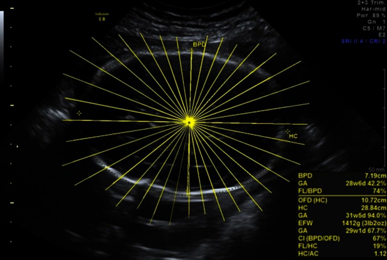
We selected the standardized cross sectional axial cranial images at the plane used to measure biparietal diameter (BPD), and performed ray analysis at the intersection between BPD and anterior–posterior diameters, to establish a consistent zero angle in all images. For each of the images, we manually measured skull diameters from center to inner skull boundary at every 10 deg for 36 spoke lengths using ImageJ,²² as shown in Fig. 6. This is currently done manually by a single reader because there are gaps in the 2-D US image where we had to interpolate where the skull boundary should be. Future work could include using a curve completing algorithm to automate measurements. As we are more interested in comparing shape deviation across all gestational ages caused by the suture malformation, we normalized the lengths for each image by the longest axis. This allows us to account for skull growth and compare across gestational ages.

Fig. 6.

Measuring the diameter of the skull at 36 angles. From the center of the skull, we follow the yellow lines to the inner skull boundary and record the distance.

3.2. Parameterization

3.2.1. Texture

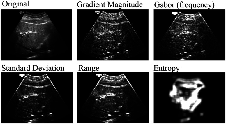
We convert each image into a feature vector by characterizing it according to its texture features at multiple scales. Our algorithm reads in each image and normalizes the pixel intensities to account for US’s settings dependence. Then it applies various 2-D image processing filters, as shown in Fig. 7, at multiple scales to highlight texture responses. Filters include standard deviation, range, and entropy each at two scale levels, as well as gradient magnitude, and total oriented wavelet response. Most of these filters measure the local rate of change in the pixel intensities, or how smooth the image is. This is relevant to steatosis because the excess fat makes the US image coarser and grainier, compared to a normal liver, which should be dark and smooth. Entropy, in contrast, works more globally to show how predictive a patch of pixels is of the whole image. Since fat build-up causes heterogeneity in livers,²³ image textures from patients with steatosis should have higher entropy.

Fig. 7.

The result of various filters applied to the liver US.

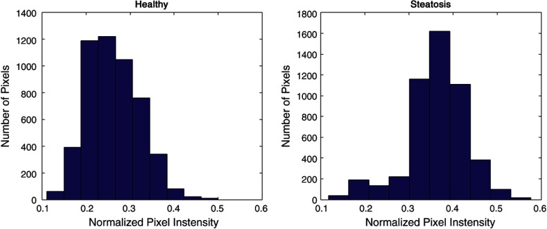
For each of the filtered responses and the unfiltered image, the algorithm extracts the pixel intensities within the ROI. It summarizes the intensities by a histogram of all the points, as shown in Fig. 8. We fit an extended Gaussian to these histograms and describe it with four parameters: mean, standard deviation, kurtosis, and skew. These four characteristics for the ROI, extracted from each of the filtered images, combine into a feature vector, summarizing the image. Through the variety of filters and with enough images, we train the classifier to generalize across variations inherent in US images such as pixel size and angle.

Fig. 8.

Histogram of pixel intensities within the ROI of on the original US image.

To evaluate which features are the most relevant, we did an exhaustive feature search using a high-performance computing cluster. This was also how we determined the window sizes of certain filters and the number of directions to use for shape analysis. These values may be adjusted depending on the clinical relative cost of false positives versus false negatives.

3.2.2. Shape

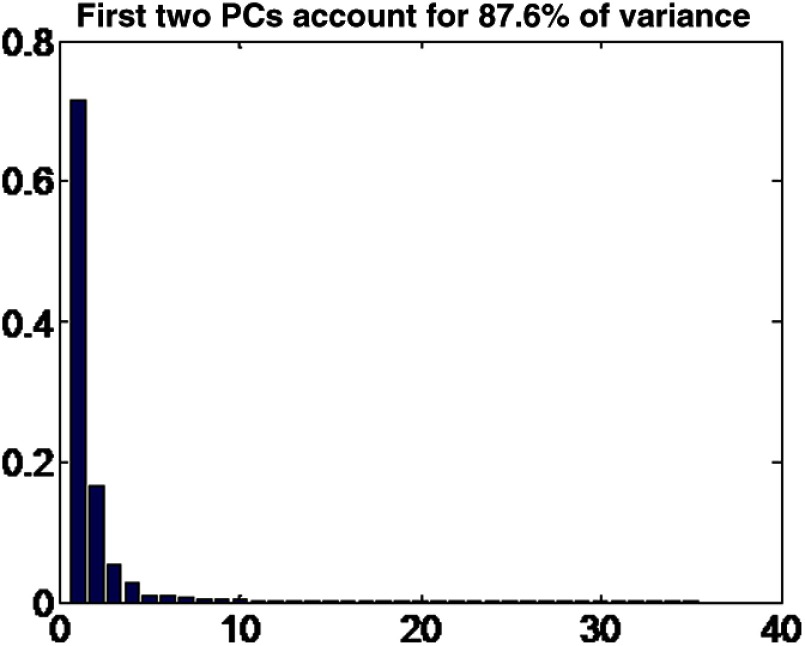
We concatenate the 36 spoke lengths into a single vector, and then use principal component analysis (PCA) on the population to reduce the dimensionality to six directions of maximum variation.²⁴ PCA finds the directions of maximum variation in the parameters and finds the component of each vector that goes in those directions. The first few directions account for most of the variance, as shown in Fig. 9.

Fig. 9.

Variance in the principal directions of the craniosynostosis dataset.

To mitigate the effect of normal variation between skull shapes and measurement error, we characterize each image by the six principal directions and discard the rest. Discarding the less relevant directions accounted for possible measurement errors from the manual measurements of the distance to the inner skull boundary.

3.3. Classification

After extracting the feature vectors, we determine their corresponding labels depending on the pathology. For steatosis, we identify 10% fat given by pathological analysis of the biopsy as a clinically relevant threshold to diagnose steatosis in previous studies.²⁵ This threshold can be adjusted for different levels of sensitivity versus specificity. Diagnosis of adenomyosis and craniosynostosis is not based on a threshold. Each is either present or not based on the diagnostic MRI and CT scans, respectively.

We then trained SVM and RF classifiers with the feature vectors and their corresponding labels for comparison of the different algorithms. We use leave-$n$-out cross-validation²⁶ to evaluate our classifiers. This means that for our test set, we took out $n$ cases. The rest were used to train the classifier, which was then tested with the $n$ cases we left out. Next, we took out a different set of $n$ cases and retrained a new classifier with the new training set to classify the new test set. We repeated this until all cases were classified and performed statistical analysis using SAS 9.4.

For steatosis, $n=2$ was selected because we wanted to have as large a training set size as possible while maintaining distinct test and training data. Since each radiologist drew an ROI for each patient, we kept both readers’ selections either in the testing set or the training set—never one in each. Thus we avoided training and testing on the same patient. We also included $n=10$ for steatosis to show the robustness of our algorithm a smaller training set.

We also trained classifiers with only the data from each of the reader to see the effect of the initial ROI selection on the classification. These results are compared to the other reader’s as well as the biopsy result and similarity is measured by kappa statistic. In the inter-rater comparison, the classifier was trained on 288 ROIs and corresponding patient images from one reader, and tested on 288 ROIs and corresponding patient images of the other. In the comparison with ground truth, leave-one-out cross-validation was used since there is one ROI per patient per reader.

For the adenomyosis and craniosynostosis study, there was one ROI and one set of measurements, respectively, for each patient, we used leave-one-out cross-validation to evaluate them. These datasets were not large enough to support leave-ten-out cross-validation.

To provide a baseline comparison for our classifier results, we asked the two radiologists who selected the ROIs for steatosis to each manually classify 51 random, blinded images from the steatosis study, and a resident to classify 102 of them. Our chart review served as our baseline comparison for the adenomyosis study. We also asked two pediatric surgeons who operate on craniosynostosis patients to classify the 44 images in the craniosynostosis study.

4. Classification Results

The results of all three studies, with both the SVM and RF classifiers for various training set sizes, are presented in Table 2.

Table 2.

The sensitivity and specificity each of the studies using different classifiers and hold-out set sizes in leave-$n$-out cross-validation obtained, along with their 95% confidence interval. It also shows statistical analysis including likelihood ratio, the area under the receiver operator characteristics curve and its confidence interval, and the $p$-value showing the likelihood of obtaining each result.

Classifier, hold-out set size	Sensitivity (%)	95% CI (%)		Specificity (%)	95% CI (%)		+LR	C-Stat	95% CI		$p$-values
Steatosis
SVM, 2	74	[68	79]	72	[67	77]	2.66	0.71	[0.67	0.74]	$<0.00010$
SVM, 10	71	[64	77]	73	[68	78]	2.61	0.70	[0.66	0.74]	$<0.0001$
RF, 2	40	[33	48]	86	[82	89]	2.90	0.67	[0.62	0.71]	$<0.0001$
RF, 10	47	[39	55]	85	[82	88]	3.19	0.69	[0.64	0.73]	$<0.0001$
Adenomyosis
SVM, 1	82	[64	92]	74	[61	84]	3.14	0.77	[0.69	0.86]	$<0.0001$
RF, 1	58	[40	74]	78	[66	86]	2.63	0.69	[0.59	0.79]	0.0012
Craniosynostosis
SVM, 1	95	[72	99]	82	[62	93]	5.25	0.89	[0.80	0.98]	0.0006
RF, 1	82	[62	93]	77	[46	93]	3.60	0.80	[0.67	0.92]	0.0037

As indicated in Table 2, SVM outperforms RF concerning sensitivity and area under receiver operating characteristic (ROC) curve (AUC) across all disease groups. SVM also slightly outperforms RF in terms of specificity for adenomyosis and craniosynostosis, though not steatosis. Specifically, RF appears to have very low sensitivity but high specificity for steatosis relative to SVM. There are some differences between hold-out size of 2 and 10, but as there is some variation training the classifier each time, even with the same dataset, the differences were not statistically significant.

Overall, RF and SVM for craniosynostosis and SVM for adenomyosis greatly outperformed all diagnostics for all other disease groups. In particular, SVM for craniosynostosis achieved a sensitivity of 95%, a positive likelihood ratio of over 5 and almost a 90% AUC value while SVM for adenomyosis and RF for craniosynostosis achieved a sensitivity of 82% and positive likelihood ratio over 3.

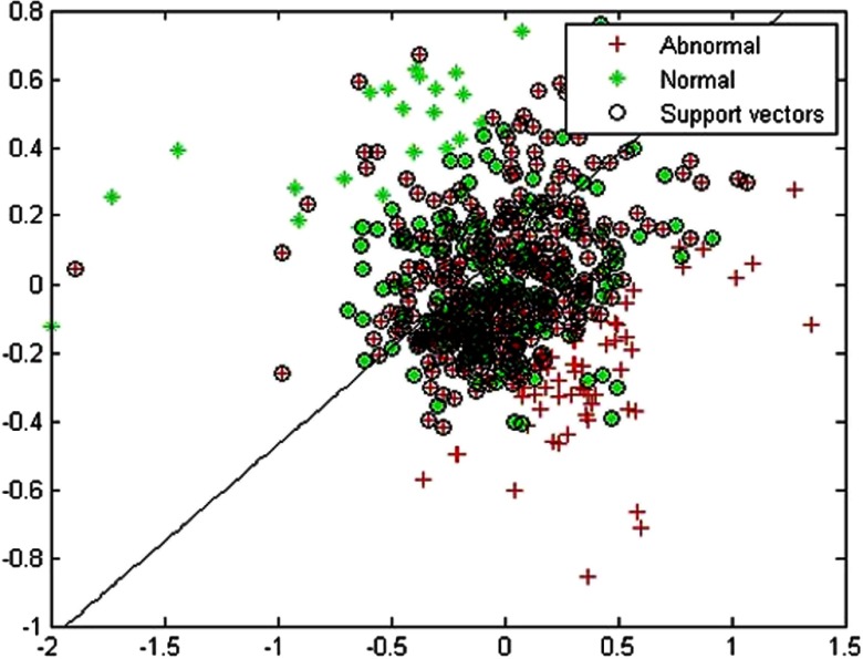
To illustrate the SVM classifier, we projected the feature vector to 2-D space using PCA in Fig. 10 to show the results of one specific training set from the steatosis study. The diagonal line shows the SVM classifier that was learned. Reducing dimensionality decreases accuracy, but even in 2-D, most of the normal cases are on one side of the line, and abnormal cases the other.

Fig. 10.

Example of a support vector machine in a 2-D projection of the high-dimensional image feature space of liver US images. The diagonal line is the classifier, where one side of the line would be classified as sick and the other as healthy.

In Fig. 11, we show two images from the steatosis data to compare a correctly classified image on the left with an incorrectly classified image on the right.

Fig. 11.

US images for steatosis. The classifier was able to successfully identify the left one but not the right.

To examine the effect of the initial ROI placement, we present the inter-reader agreement in Table 3 where the classifier was trained on one of the reader’s ROI and tested on another’s. Table 4 shows the results when each reader’s classifier compared to ground truth.

Table 3.

Inter-reader agreement for steatosis study.

	Agreement	95% CI		$p$-values
Reader 1 * Reader 2, SVM	$K=0.1321$	[0.0175	0.2468]	$<0.001$
Reader 1 * Reader 2, RF	$K=0.1342$	[0.0106	0.2578]	$<0.001$

Table 4.

Classification results from individual readers for steatosis compared with ground truth. All tests used leave-one-out cross-validation.

	Classifier	Agreement	95% CI		Sensitivity (%)	Specificity (%)	ROC (%)	$p$-values
Reader 1 * Truth	SVM	$K=0.3410$	[0.2336	0.4485]	69.2	68.0	0.67	$<0.001$
Reader 2 * Truth	SVM	$K=0.3504$	[0.2401	0.4607]	64.9	72.2	0.67	$<0.001$
Reader 1 * Truth	RF	$K=0.3909$	[0.2769	0.5050]	46.8	89.2	0.73	$<0.001$
Reader 2 * Truth	RF	$K=0.2836$	[0.1662	0.4011]	42.6	84.0	0.66	$<0.001$

Inter-reader agreement between readers was poor, as indicated by very low Kappa values. Compared with the pathological results from biopsy, sensitivity was higher for readers ROIs when using SMV relative to RF, though specificity suffered.

As a baseline comparison, the same expert radiologists who identified the ROI manually for steatosis rated 51 random images from this study each, and obtained 84% and 71% accuracy. This was considerably higher than a resident, who rated 102 images for an accuracy of 49%. In a similar study with craniosynostosis, we asked two expert physicians to rate our 44 cases for craniosynostosis and control. They obtained 45% and 50% accuracy. For adenomyosis, our chart review found 75% false negative rates, which is in line with the low sensitivity from transabdominal US in previous work.¹¹

5. Evaluation and Discussion

We present a novel, validated, and flexible framework for quantitative image analysis using clinical US data. Over all trials, our system achieved accuracy of 72.74% and AUC of 0.71 for steatosis, 77.27% and 0.77 for adenomyosis, and 88.63% and 0.89 for craniosynostosis in predicting the presence of specific diseases. Our framework’s accuracy is near that of expert readers for a steatosis, and greatly exceeds the sensitivity of standard clinical diagnosis of adenomyosis and craniosynostosis.

We propose that our framework could help nonexpert readers correctly classify liver US and flag images that are suspicious for adenomyosis and craniosynostosis that would otherwise be missed. Identifying steatosis earlier could prevent more severe symptoms, identifying adenomyosis could help more patients get treated for it, and identifying at-risk cases of craniosynostosis earlier could help with treatment planning and parent counseling.¹⁷

From our results comparing the initial ROI selection for steatosis, although both readers’ ROIs led to similar performance compared with the ground truth, they had poor agreement with each other. This suggests that the framework can learn the features each reader looked for, but cannot generalize across readers. Thus, the readers selecting the test ROIs should be the same was the ones provide the training ROIs. Future work could examine whether having training ROIs from more readers could increase the robustness of the algorithm for testing ROIs from a new reader.

Similar texture analysis based metrics have been applied to smaller, experimental settings.^4,7,21,27 Because this is a general framework, we were able to combine many of the features identified in literature as relevant for diagnosing steatosis. For example, we incorporated standard deviation as a feature similar to what Lee et al.⁸ proposed, and Gabor filters²⁸ to look at the frequency components noted by Wu et al.⁶ With our larger feature set, we were able to demonstrate better separation between normal and abnormal than with using standard deviation alone, and our large study size establishes the statistical significance of the differences in frequency energy content.

In testing the different classifiers, we found that the SVM gives the better balance between accuracy, sensitivity, and specificity through AUC analysis using MATLAB 2015a. RF sometimes gave better accuracy overall but a worse trade-off between sensitivity and specificity as shown by the smaller AUC. Depending on the application and which is more clinically costly, the different classifiers provide the ability to preferentially target either sensitivity or specificity.

Compared to previous works, our study presents a more general framework tested on a larger and more heterogeneous dataset. We were unable to match Minhas et al.’s⁴ accuracy of 80.68% in identifying steatosis. The difference could be from the more heterogeneous dataset with variability in machine settings and operators, or from using biopsy results for labels instead of human readers. Whereas Lee et al.’s⁸ study showed that the ranges of both the mean and the standard deviation of the pixel intensity histogram overlapped significantly, we have shown that these features along with others can be used to classify the two groups. For the adenomyosis study, we have shown that our computer-aided diagnosis framework using pelvic US matches the accuracy of expert readers with transvaginal US.¹³ Lastly, our craniosynostosis results show that shape analysis can be used to classify nonsyndromic forms of the disease with high accuracy in the general population, and not just the high-risk ones as identified by Delahaye et al.¹⁴

Future work includes implementing an image normalization technique to explicitly learn the properties of the uncalibrated US data. Currently, we implicitly learn which properties are important through separating the parameters, but better normalization techniques that incorporate additional information could explicitly account for expected variations in the dataset. For example, physicians often compare liver to kidney US when looking for hepatic steatosis. The kidney gives the patient-specific baseline echo-texture response. This could be quantified and subtracted from the liver features to examine only the deviation from baseline for each patient.

Our extensible feature set allows for the incorporation of additional features, such as elastography scores. We used general features and filters to show the adaptability of our framework, but more sophisticated filters targeting specific diseases, or more complex machine-learning algorithms like neural networks could be incorporated.

Lastly, parallelizing the framework to run on high-performance computing clusters and mapping it to hardware accelerators like GPU could significantly improve runtime for training. Currently, we use trivial parallelization and run multiple instances of on different nodes to search through the parameter space, but this does not improve the runtime of a single instance. The improvement in runtime would become more important in extending our framework to more data-intensive problems like working directly with the data-stream off the US machine rather than the filtered images it displays.

6. Conclusion

We achieved consistent results across all three clinical targets collected across 5 years at different US settings, by different operators, and from multiple disease sites. This suggests that our framework is reliable, flexible, and effective enough that it will be suitable for clinical application with routinely collected images. Our framework could be used to aid clinical decision making and give physicians more confidence in their diagnoses or lack of. With more cases, especially for adenomyosis and craniosynostosis, and further refinement in feature selection and the learning process, we hope to increase confidence in our results and include it as a standard routine in the clinic.

Biographies

Jie Ying Wu is an applied math master’s student at the Centrale Supélec in Paris. She received her BSc degree in computer engineering from Brown University. While there, she worked at the Rhode Island Hospital, doing research in medical image analysis. She is interested in applying technology to healthcare and is pursuing a PhD in medical robotics.

Adam Tuomi is a medical student at the Alpert Medical School of Brown University. As an undergraduate, also at Brown University, he concentrated in mathematics and physics. Always looking to combine his interests in medicine and the quantitative sciences, he pursues research in computer-aided diagnosis and medical image analysis.

Michael D. Beland is an associate professor of diagnostic imaging at Brown University. He is medical director of the Ultrasound Department at the Rhode Island Hospital and Rhode Island Medical Imaging specializing in ultrasound imaging. He has over 50 publications, over 50 scientific presentations, numerous invited speaking events and several grants. His areas of interest include diagnostic and interventional ultrasound, elastography, contrast ultrasound, advanced fusion imaging, body CT/MRI, and prostate MRI.

Joseph Konrad is a fourth-year diagnostic radiology resident at Brown University who will be pursuing a fellowship in interventional radiology at UCLA in 2016.

David Glidden is a medical student at the Warren Alpert Medical School at Brown University. He received his undergraduate degree in computer science and biology from Northeastern University. He has worked at multiple startups prior to attending medical school.

David Grand is a graduate of Mount Sinai School of Medicine and did his postdoctoral training in MRI at the Johns Hopkins Hospital. He is the director of body MRI at the Rhode Island Hospital and is an associate professor of diagnostic imaging at the Warren Alpert Medical School of the Brown University.

Derek Merck received his PhD in computer science at the University of North Carolina, where he developed methods for statistical shape analysis and radiation-treatment planning. His research is focused on medical image analysis and visualization. He is currently the director of computer vision and image analysis at Rhode Island Hospital and an assistant professor of diagnostic imaging, radiation-oncology, and engineering at Brown University. Prior to his academic career, he worked as a professional software architect.

References

- 1.Vicas C., et al. , “Influence of expert-dependent variability over the performance of noninvasive fibrosis assessment in patients with chronic hepatitis C by means of texture analysis,” Comput. Math. Methods Med. 2012, 1–9 (2012). 10.1155/2012/346713 [DOI] [PMC free article] [PubMed] [Google Scholar]
- 2.Browning J. D., et al. , “Prevalence of hepatic steatosis in an urban population in the United States: impact of ethnicity,” Hepatology 40, 1387–1395 (2004). 10.1002/hep.20466 [DOI] [PubMed] [Google Scholar]
- 3.Hamer O. W., et al. “Fatty liver: imaging patterns and pitfalls,” RadioGraphics 26, 1637–1653 (2006). 10.1148/rg.266065004 [DOI] [PubMed] [Google Scholar]
- 4.Minhas F., Sabih D., Hussain M., “Automated classification of liver disorders using ultrasound images,” J. Med. Syst. 36, 3163–3172 (2012). 10.1007/s10916-011-9803-1 [DOI] [PubMed] [Google Scholar]
- 5.Thijssen J. M., et al. , “Computer-aided B-mode ultrasound diagnosis of hepatic steatosis: a feasibility study,” IEEE Trans. Ultrason. Ferroelectr. Freq. Control 55, 1343–1354 (2008). 10.1109/TUFFC.2008.797 [DOI] [PubMed] [Google Scholar]
- 6.Wu C.-M., Chen Y.-C., Hsieh K.-S., “Texture features for classification of ultrasonic liver images,” IEEE Trans. Med. Imaging 11, 141–152 (1992). 10.1109/42.141636 [DOI] [PubMed] [Google Scholar]
- 7.Khoo B. C. C., McQueen M. P. C., Sandle W. J., “Use of texture analysis to discriminate between normal livers and livers with steatosis,” J. Biomed. Eng. 13, 489–494 (1991). 10.1016/0141-5425(91)90096-P [DOI] [PubMed] [Google Scholar]
- 8.Lee C. H., et al. , “Usefulness of standard deviation on the histogram of ultrasound as a quantitative value for hepatic parenchymal echo texture; preliminary study,” Ultrasound Med. Biol. 32, 1817–1826 (2006). 10.1016/j.ultrasmedbio.2006.06.014 [DOI] [PubMed] [Google Scholar]
- 9.Taran F. A., Stewart E. A., Brucker S., “Adenomyosis: epidemiology, risk factors, clinical phenotype and surgical and interventional alternatives to hysterectomy,” Geburtshilfe Frauenheilkd. 73, 924–931 (2013). 10.1055/s-0033-1350840 [DOI] [PMC free article] [PubMed] [Google Scholar]
- 10.Dueholm M., “Transvaginal ultrasound for diagnosis of adenomyosis: a review,” Best Pract. Res. Clin. Obstet. Gynaecol. 20, 569–582 (2006). 10.1016/j.bpobgyn.2006.01.005 [DOI] [PubMed] [Google Scholar]
- 11.Bazot M., et al. , “Ultrasonography compared with magnetic resonance imaging for the diagnosis of adenomyosis: correlation with histopathology,” Hum. Reprod. 16, 2427–2433 (2001). [DOI] [PubMed] [Google Scholar]
- 12.Kunz G., et al. , “Adenomyosis in endometriosis—prevalence and impact on fertility: evidence from magnetic resonance imaging,” Hum. Reprod. 20, 2309–2316 (2005). 10.1093/humrep/dei021 [DOI] [PubMed] [Google Scholar]
- 13.Kepkep K., et al. , “Transvaginal sonography in the diagnosis of adenomyosis: which findings are most accurate?” Ultrasound Obstet. Gynecol. 30, 341–345 (2007). 10.1002/uog.3985 [DOI] [PubMed] [Google Scholar]
- 14.Delahaye S., et al. , “Prenatal ultrasound diagnosis of fetal craniosynostosis,” Ultrasound Obstet. Gynecol. 21, 347–353 (2003). 10.1002/uog.91 [DOI] [PubMed] [Google Scholar]
- 15.Slater B. J., et al. , “Cranial sutures: a brief review,” Plast. Reconstr. Surg. 121, 170e–178e (2008). 10.1097/01.prs.0000304441.99483.97 [DOI] [PubMed] [Google Scholar]
- 16.Persing J. A., “MOC-PS(SM) CME article: management considerations in the treatment of craniosynostosis,” Plast. Reconstr. Surg. 121, 1–11 (2008). 10.1097/01.prs.0000305929.40363.bf [DOI] [PubMed] [Google Scholar]
- 17.Fearon J. A., “Evidence-based medicine: craniosynostosis,” Plast. Reconstr. Surg. 133, 1261–1275 (2014). 10.1097/PRS.0000000000000093 [DOI] [PubMed] [Google Scholar]
- 18.Miller C., et al. , “Ultrasound diagnosis of craniosynostosis,” Cleft Palate. Craniofac. J. 39, 73–80 (2002). [DOI] [PubMed] [Google Scholar]
- 19.Cortes C., Vapnik V., “Support-vector networks,” Mach. Learn. 20, 273–297 (1995). [Google Scholar]
- 20.Breiman L., “Random forests,” Mach. Learn. 45, 5–32 (2001). 10.1023/A:1010933404324 [DOI] [Google Scholar]
- 21.Li G., et al. , “Computer aided diagnosis of fatty liver ultrasonic images based on support vector machine,” in 30th Annual Int. Conf. of the IEEE Engineering in Medicine and Biology Society (EMBS), pp. 4768–4771 (2008). 10.1109/IEMBS.2008.4650279 [DOI] [PubMed] [Google Scholar]
- 22.Schneider C. A., Rasband W. S., Eliceiri K. W., “NIH Image to ImageJ: 25 years of image analysis,” Nat. Methods 9, 671–675 (2012). 10.1038/nmeth.2089 [DOI] [PMC free article] [PubMed] [Google Scholar]
- 23.Bedossa P., Dargere D., Paradis V., “Sampling variability of liver fibrosis in chronic hepatitis C,” Hepatology 38, 1449–1457 (2003). 10.1016/j.hep.2003.09.022 [DOI] [PubMed] [Google Scholar]
- 24.Cootes T. F., Edwards G. J., Taylor C. J., “Active appearance models,” in Computer Vision—ECCV’98, Burkhardt H., Neumann B., Eds., pp. 484–498, Springer, Berlin Heidelberg: (1998), http://link.springer.com/chapter/10.1007/BFb0054760 [Google Scholar]
- 25.Castera L., et al. , “Worsening of steatosis is an independent factor of fibrosis progression in untreated patients with chronic hepatitis C and paired liver biopsies,” Gut 52, 288–292 (2003). 10.1136/gut.52.2.288 [DOI] [PMC free article] [PubMed] [Google Scholar]
- 26.Duda R. O., Hart P. E., Stork D. G., Pattern Classification, John Wiley & Sons, New York: (2012). [Google Scholar]
- 27.Horng M.-H., “An ultrasonic image evaluation system for assessing the severity of chronic liver disease,” Comput. Med. Imaging Graph. 31, 485–491 (2007). 10.1016/j.compmedimag.2007.05.001 [DOI] [PubMed] [Google Scholar]
- 28.Fogel I., Sagi D., “Gabor filters as texture discriminator,” Biol. Cybern. 61, 103–113 (1989). 10.1007/BF00204594 [DOI] [Google Scholar]