Improving power and accuracy of genome-wide association studies via a multi-locus mixed linear model methodology

Abstract

Genome-wide association studies (GWAS) have been widely used in genetic dissection of complex traits. However, common methods are all based on a fixed-SNP-effect mixed linear model (MLM) and single marker analysis, such as efficient mixed model analysis (EMMA). These methods require Bonferroni correction for multiple tests, which often is too conservative when the number of markers is extremely large. To address this concern, we proposed a random-SNP-effect MLM (RMLM) and a multi-locus RMLM (MRMLM) for GWAS. The RMLM simply treats the SNP-effect as random, but it allows a modified Bonferroni correction to be used to calculate the threshold p value for significance tests. The MRMLM is a multi-locus model including markers selected from the RMLM method with a less stringent selection criterion. Due to the multi-locus nature, no multiple test correction is needed. Simulation studies show that the MRMLM is more powerful in QTN detection and more accurate in QTN effect estimation than the RMLM, which in turn is more powerful and accurate than the EMMA. To demonstrate the new methods, we analyzed six flowering time related traits in Arabidopsis thaliana and detected more genes than previous reported using the EMMA. Therefore, the MRMLM provides an alternative for multi-locus GWAS.

Genome-wide association studies (GWAS) have been widely used in genetic dissection of complex traits, especially with the development of advanced genomic sequencing technologies. The mixed linear model (MLM) method¹,² by fitting a population structure (Q) and a polygene (K), the so called Q + K model, is the most popular method used for GWAS. After the MLM of Yu et al.² was published, many advanced MLM-based methods have been proposed³,⁴,⁵,⁶,⁷, primarily to improve computational efficiency. A common feature of the MLM based GWAS is the one-dimentional genome scan by testing one marker at a time. The major advantage of such a genome scanning approach is the ability to handle a large number of markers, e.g., more than a million markers. However, such a model does not facilitate good estimates of marker effects because the model is never correct if a trait is indeed controlled by multiple loci, which is the case for most complex traits. Another problem with the method is the issue of multiple test correction for the threshold value of significance test. The typical Bonferroni correction is often too conservative, so that many important loci may not pass the stringent criterion of significance test.

Most complex traits are controlled by several major loci plus numerious undetectable loci with small effects (collectively called polygenes). The one-dimentional scanning GWAS will never recover the true model due to the intrinsic limitation of the model. Multi-locus models are better alternative methods for GWAS; these include Bayesian LASSO⁸, penalized Logistic regression⁹,¹⁰, Elastic-Net¹¹, and empirical Bayes¹² methods. An obvious advantage of these methods is that no Bonferroni correction is required because of the multi-locus nature. Although these methods are shrinkage approaches and are supposed to be able to handle the number of markers several times larger than the sample sizes, they will fail when the number of markers is many times larger than the sample size, either due to constraint in computational time or limit in memory allocation. These models will also face the multicollinearity issue when the marker density is extremely high. Recently, Segura et al.¹³ has proposed a multi-locus MLM approach. However, further refinement is needed.

If the number of markers is small or moderately large and can be handled by one of the multi-locus approaches, we should consider a multi-locus method for GWAS, otherwise, a combination of the single locus genome scanning and multiple locus analysis may be considered. In the first stage, markers are scanned and selected with a low criterion of significance test. In the second stage, a multiple locus method is implemented for markers that have passed the initial screening. Statistical tests and marker effect estimation are then based on the multiple locus model. The MLM method of GWAS in the initial scanning stage treats marker effects as fixed. Goddard et al.¹⁴ proposed to treat marker effects as random, following a normal distribution with zero mean and an unknown variance. They described several advantages of the random model approach over the fixted model treatment. One advantage is that the random model approach will shrink the estimated (better called predicted) marker effects towards zero, leading to a maximum correlation between observed and predicted phenotypic values. However, Goddard et al.¹⁴ did not provide an efficient computational algorithm to estimate (or predict) marker effects.

In this study, we developed an efficient algorithm to estimate variances of the markers and predict effects of these markers. This method is called the random-SNP-effect mixed linear model (RMLM). The result of RMLM can either be treated as the final result of GWAS or used to select markers for the second stage analysis. In the second stage of GWAS, the selected markers are simultaneously evaluated in a single model using an EM empirical Bayes approach¹⁵. Estimation of marker effects and significance tests of these markers are performed in the second stage. This method is called the multi-locus random-SNP-effect mixed linear model (MRMLM). We demonstrate that this two-stage combined method of GWAS has significantly increased the statistical power and decreased Type 1 error compared with other methods, including the efficient mixed model analysis (EMMA).

Results

Statistical power for quantitative trait nucleotide (QTN) detection

To confirm the effectiveness of the MRMLM and RMLM methods, a series of Monte Carlo simulation experiments were carried out. Each sample was analyzed by the two new methods (MRMLM and RMLM) along the EMMA method. The significance threshold p value for the MRMLM method was 0.0002 (see Methods for calculation of this threshold). The corresponding threshold p value for the RMLM method was (modified Bonferroni correction for multiple tests), where is the effective number of markers (see Methods for calculation of m_e). The threshold p value for the EMMA method was (Bonferroni correction for multiple tests), where m is the total number of markers. For each QTN, power was defined as the proportion of samples where the QTN was detected (p value smaller than the designated threshold). In the first simulation experiment where no polygenic variance was simulated, the MRMLM method has the highest power for all six QTNs simulated, followed by the RMLM method and the EMMA method (Fig. 1a and Table S1). On one occasion (QTN number 5), the RMLM method is slightly more powerful than the MRMLM method. In the second simulation experiment when an additive polygenic variance ( and ) was added to the polygenic background, the same trend in power was observed where MRMLM is more powerful than RMLM and EMMA is the least powerful (Fig. 1b and Table S2). On one occasion (QTN number 4), the three methods have very similar power, with RMLM being slightly more powerful than the other two methods. In the third simulation experiement where three pairs of epistatic effects (collectively contributing 0.15 of the phenotypic variance) was added to the genetic background, again, MRMLM is the most powerful followed by RMLM and EMMA (Fig. 1c and Table S3) with an exception for QTN number 5 where RMLM is slightly more powerful than MRMLM. The sample sizes of the above three simulation experiments were all . We also changed the sample size from 199 to 149 and 99 under the fourth simulation experiment with the MRMLM method. The statistical powers are demonstrated in Fig. 1(d). As expected, the statistical power has declined as we reduced the sample size (Table S4). Similar trend of power changes were also observed for different numbers of markers (Table S5).

Figure 1. Comparison of statistical powers of six simulated QTN from three different methods of GWAS (MRMLM, RMLM and EMMA).

Panel (a) no polgenic variance was simulated. Panel (b) an additive polygenic variance (explaining 0.092 of the phenotypic variance) was simulated. Panel (c) three epistatic QTNs each explaining 0.05 of the phenotypic variance were simulated. Panel (d) powers of six simulated QTNs with an additive polygenic variance obtained from the MRMLM method under three different sample sizes (199, 149 and 99).

Accuracies of estimated QTN effects

We used the mean squared error (MSE) to measure the accuracy of an estimated QTN effect for a particular method. We evaluated the accuracies for all the six simulated QTNs from all three methods. The MSE’s are demonstrated in Fig. 2, where panels (a), (b) and (c) represent the results from the three simulation experiments, respectively. The MRMLM method is consistently more accurate than the RMLM method, which in turn is more accurate than the EMMA method (see Tables S1–S3). Figure 2(d) shows the results of different sample sizes by the MRMLM method from the fourth simulation experiment, showing that, as expected, a large sample size is associated with a small MSE (Table S4).

Figure 2. Comparison of mean squared errors of six simulated QTNs from three different methods of GWAS (MRMLM, RMLM and EMMA).

Panel (a) no polgenic variance was simulated. Panel (b) an additive polygenic variance was simulated. Panel (c) three epistatic QTNs were simulated. Panel (d) mean squared errors of six simulated QTNs with an additive polygenic variance obtained from the MRMLM method under three different sample sizes (199, 149 and 99).

Type 1 error and ROC curve

The empirical Type 1 error rates of the three methods from the three simulation experiments are illustrated in Fig. 3. Overall, the three methods have similar Type 1 errors except the first simulation experiment where EMMA has an very large Type 1 error compared with the two new methods. In the second and third simulation experiments, EMMA has the least Type 1 errors followed by the MRMLM and RMLM methods. Fig. 3(d) shows the empirical Type 1 errors of the MRMLM method from the fourth simulation experiment with three different sample sizes (199, 149 and 99), where Type 1 error has been increased with a decreased sample size.

Figure 3. Comparison of empirical Type 1 error rates from three different methods of GWAS (MRMLM, RMLM and EMMA).

Panel (a) no polgenic variance was simulated. Panel (b) an additive polygenic variance was simulated. Panel (c) three epistatic QTNs were simulated. Panel (d) empirical Type 1 error rates obtained from the MRMLM method under three different sample sizes (199, 149 and 99).

A useful way to compare different methods for their efficiencies in the detection of significant effects is the receiver operating characteristic (ROC) curve comparison. An ROC is a plot of the statistical power against the controlled Type 1 error. The higher the curve, the better the method. When sixty-one probability levels for significance, between 1E-8 to 1E-2, were inserted, the corresponding powers were calculated in the first simulation experiment. Figure 4 shows the comparison of the ROC curves from the three methods for each of the six QTNs simulated from the first simulation experiment. Clearly, the MRMLM method stands out way above the other two methods while the RMLM is better than the EMMA method when the Type 1 error is relaxed.

Figure 4. Statistical powers of six simulated QTNs from the first simulation experiement plotted against Type 1 error (in a log₁₀ scale) for the three GWAS methods (MRMLM, RMLM and EMMA).

Computational efficiency

When performing GWAS on the simulated data, we first scanned the genome by the single-locus RMLM method to find the association between each SNP and the trait of interest. This process took 12.78 hours (Intel Core i5 CPU 4570, 3.20 GHz, Memory 8.00G, 1000 datasets) in the first simulation experiment. The MRMLM took an additional 0.51 hours to conduct the multi-locus analysis. Although the MRMLM method requires more computing time, the high power and small MSE relative to the RMLM method are good justifications for the improved method. The EMMA method took 68.77 hours for completing the analysis for the first simulation experiment.

Real data analyses in Arabidopsis

We analyzed six flowering time related traits of the Arabidopsis thaliana population published by Atwell et al.¹⁶ using all the three methods (MRMLM, RMLM and the EMMA). The numbers of SNPs significantly associated with the six traits are 29, 15, 27, 13, 22 and 14, respectively, for traits LD (days to flowering under long days), LDV (days to flowering under long days with vernalization), SD (days to flowering under short days), 0 W (days to flowering under long days with no vernalization), 2 W (days to flowering under long days for two week vernalization) and 4 W (days to flowering under long days for four week vernalization), from the MRMLM method. The corresponding numbers of associated SNPs are 8, 5, 3, 6, 6 and 7 from the RMLM method. The EMMA method only detected 1, 3, 1, 0, 1 and 2 SNPs for the above six traits (see Table S6 for details of the associated SNPs). These significantly associated SNPs for each trait were used to conduct a multiple linear regression analysis and the corresponding Bayesian information criteria (BIC) were calculated. The MRMLM method shows the lowest BIC values for all traits (Table 1), indicating that SNPs detected by the MRMLM method fit the data better than the other methods.

Table 1. Goodness of fit (log likelihood and BIC) for SNPs detected by three methods (MRMLM, RMLM and EMMA), where a lower value indicates a better fit.

Traita	−Log likelihood value			Bayesian information criterion (BIC)
	MRMLM	RMLM	EMMA	MRMLM	RMLM	EMMA
LD	−215.9	153.8	284.6	−67.5	194.8	289.7
SDV	−337.2	−150.1	−119.9	−260.4	−124.5	−104.5
SD	−367.9	55.3	113.1	−230.5	70.5	118.2
0W	−42.4	94.5	226.2	21.5	124.0	226.2
2W	−140.6	104.4	216.4	−30.1	134.6	221.4
4W	−122.4	24.5	105.3	−55.5	57.9	114.9

^aLD: days to flowering under long days; LDV: days to flowering under long days with vernalization; SD: days to flowering under short days; 0W: days to flowering under long days for no vernalization; 2W: days to flowering under long days for 2 weeks vernalization; 4W: days to flowering under long days for 4 weeks vernalization.

We found that 6, 4, 6, 2, 3 and 5 genes previously reported to be associated with the six traits are in the proximity of the SNPs detected by the MRMLM method. The corresponding numbers of genes in the vicinity of the SNPs detected by the RMLM method are 3, 3, 2, 1, 1 and 2, respectively, for the six traits. Only 2, 2, 1, 0, 0 and 1 genes are in the neighborhood of the SNPs detected by the EMMA method (see Table 2 and Table S7 for details of the genes). Clearly, the MRMLM method detected more known genes than the other two methods, indicating that this multi-locus model (MRMLM) has a higher power for QTN detection than the single-locus model (RMLM) and the EMMA method.

Table 2. Genes detected for six flowering time traits in Arabidopsis thaliana using three methods (MRMLM, RMLM and EMMA).

Trait	Gene detected	Chr	SNP (bp)	MRMLM			RMLM			EMMA			Reference
				LOD	Effect	r2(%)	P-value	Effect	r2(%)	P-value	Effect	r2(%)
LD	AT1G23000	1	8128350	4.12	−0.055	0.56
	SVP	2	9588685				4.47E-10	−0.397	23.36	2.78E-9	−0.407	24.59	18
	AGL17	2	9611587	8.83	−0.104	1.67	7.11E-7	−0.262	10.56				19
	ETC3	4	454542	4.70	−0.066	0.72							20
	GA1	4	1260796	3.06	−0.059	0.63							21
	AT4G14385	4	8291057	6.18	−0.060	0.66
	FLC	5	3188328	9.48	−0.097	1.35	5.08E-7	−0.248	8.73	8.82E-7	−0.258	9.45	22
LDV	CENH3	1	164375	6.30	−0.049	3.37
	SVP	2	9588685	10.30	−0.049	2.98	1.61E-6	−0.111	15.43				18
	CKB4	2	18446546	5.75	−0.053	2.05	2.66E-8	−0.152	16.80	5.74E-8	−0.158	18.15	23
	DOG1	5	18599929	7.25	−0.058	4.77	2.04E-7	−0.083	9.82	2.71E-7	−0.087	10.87
SD	AT1G52930	1	19713470	6.21	−0.049	1.27
	HEN2	2	2916675	3.83	0.030	0.53
	EDA8	4	153402	6.47	−0.042	1.13	2.46E-8	−0.132	11.26	6.74E-8	−0.136	12.00
	ETC3	4	458226	10.70	−0.070	2.03	1.20E-6	−0.132	7.18				20
	IDL3	5	3051259	6.23	−0.037	0.87
	AT5G19430	5	6546055	4.66	−0.068	1.36
0W	AGL18	3	21239134	6.24	−0.111	3.13							24
	DOG1	5	18592535				1.83E-6	−0.274	12.72
	DOG1	5	18595015	11.87	−0.145	3.56
2W	ANP1	1	2899659	8.11	−0.081	1.55
	ETC3	4	454542	7.18	−0.089	1.72	4.30E-7	−0.207	9.21				20
	DCL4	5	6846957	3.36	−0.082	0.99
4W	ATPERK12	1	8341601	4.65	−0.070	1.34
	SVP	2	9588685				3.55E-9	−0.354	28.25	1.97E-8	−0.365	30.03	18
	AT2G30600	2	13031229	9.65	−0.107	3.00
	C3HC4	5	6546259	5.94	−0.132	2.75
	AT5G45190	5	18264316	7.06	−0.071	1.33
	DOG1	5	18607728	10.09	−0.164	4.69	8.13E-7	−0.263	12.09

r²: Proportion of phenotypic variance contributed by the gene.

Discussion

To reduce computing time required for GWAS, Zhang et al.⁶ proposed a P3D algorithm that fixes the polygenic-to-residual variance ratio in the genome-wide scanning step. Kang et al.³ used a matrix transformation prior to the genome-wide scanning stage and treated the scanned SNP effect as fixed. If we view the SNP effect as random, one additional variance of the QTN effect needs to be estimated, and the complexity and computing time in parameter estimation has been increased, as shown with the MLM-based approaches of Zhang et al.¹ and Yu et al.². In the present study, a new matrix transformation is constructed, the P3D algorithm is adopted, and the residual variance is estimated after the variance of the QTN effect is estimated. Therefore, only one parameter, the ratio of the QTN effect variance to the residual variance, is estimated in the genome-wide scanning stage. In doing so, the MRMLM method requires only 20% of the computing time needed by the EMMA method. More importantly, the new method performs better than EMMA in terms of high statistical power, low Type 1 error and low MSE of an estimated QTN effect.

The current GWAS method is a single-locus analysis approach under polygenic background and population structure controls. The number of tests involved is the number of markers, requiring a Bonferroni correction for multiple tests. To control the experimental error at a genome-wide level of 0.05, the significance level for each test should be adjusted as , which is 5E-8 if one million markers are to be scanned. In the multi-locus model, however, there is no need for such a multiple test correction due to the multi-locus and shrinkage natures of the new method. This conclusion is also supported by the results of Monte Carlo simulation studies. We compared the result of EMMA in this study with the result reported in Atwell et al.¹⁶; fewer known genes are listed in Table 2, because some genes identified in previous studies are not significantly associated with the traits after the Bonferroni correction. If the significance level was changed to a less stringent criterion, more known genes would have been found (Table S7). We investigated the effect of the critical value on the selection of putative QTNs. Similar results were observed for the three critical values selected (0.001, 0.01 and 0.05), although the 0.01 value resulted in the marginally best performance in terms of statistical power of QTN detection and accuracy of QTN effect estimation (Table S8).

There are several multi-locus GWAS approaches already published in the literature⁵,¹³,¹⁷. When the number of markers is not large, all marker effects and their interactions can be included in a single model, such as the empirical Bayes method¹². If the number of markers is large, this single model approach is not feasible. One question is how to reduce the number of parameters in a full genetic model. Zhou et al.⁵ developed a Bayesian sparse linear mixed model and Moser et al.¹⁷ proposed a Bayesian mixture model. Under these models, two to four common components in the mixture distribution were considered and only a few variance components were estimated. Although about 500 effects in the genetic model are finally considered after several rounds of Gibbs sampling, the computing time becomes a major concern for these Bayesian approaches. Therefore, the ideal method is to delete spurious QTN effects prior to implementing the multi-locus model. The first step of MRMLM is RMLM, which deletes the majority of the markers in advance so that only a small set of markers are left to the second stage for evaluation. The MRMLM method differs from the multi-locus method of Segura et al.¹³ in several aspects. First, the SNP effects are viewed as random in the MRMLM method while they are treated as fixed effects in Segura et al.¹³. Secondly, we adopted a simple matrix transformation technique to improve the computational efficiency while Segura et al.¹³ implemented an algorithm involving three complicated treatments. Finally, the MRMLM method uses one set of selected SNPs, which have p values less than 0.01 in the initial scanning while Segura et al.¹³ requires MCMC samplings.

Atwell et al.¹⁶ listed 500 most significantly associated SNPs, although some of them were not significant at the criterion. In the neighborhood of these SNPs, some genes were found to be related to the traits of interest (Table 2 and S7). In this study, 21 genes for six flowering time traits are found to be in the vicinity of the detected SNPs, consistent with results previously reported, as shown in the database ( http://www.arabidopsis.org/), the work of Atwell et al.¹⁶ and related references18,19,20,21,22,23,24 (Table S7). Therefore, the Arabidopsis thaliana GWAS results of his study appear to be reliable.

In the study of GWAS methodology, real genotypes in natural population are frequently used to conduct Monte Carlo simulation studies¹,²,⁶. In this study, therefore, the real SNP dataset in Atwell et al.¹⁶ was adopted in the simulation studies. To further confirm the new methods, 200 samples with simulated genotypes derived from the minPtest R package²⁵ were analyzed. As a result, similar results were found (Table S9).

Conclusion

The RMLM simply treats the SNP effect as random, and includes new matrix transformation, fixing the polygenic-to-residual variance ratio and estimating residual variance after the variance of QTN effect is obtained. Meanwhile, it allows a modified Bonferroni correction to be used to calculate the threshold p value for significance tests. The MRMLM is a multi-locus model including markers selected from the RMLM, and all the effects in the model are estimated by an EM empirical Bayes method. Results from real data analyses and simulation studies show that the MRMLM has the highest power for QTN detection, the best fit for genetic model, the minimal bias in the estimation of the QTN effect, and the strongest robustness, as compared with the RMLM and the EMMA.

Methods

Random effect linear mixed model (RMLM)

Let y be a vector of phenotypic values for all individuals. The mixed linear model is

where X is an incident matrix for fixed (non genetic) effects, is a vector of the fixed effects, is a vector of genotype indicators for the kth SNP that are coded as 1, 0 and −1, for one of the two homozygotes, the heterozygote and the other homozygote, respectively, is the effect of marker k with an assumed normal distribution of mean zero and variance , is a vector of polygenic effects with a multivariate normal distribution of mean zero and variance described by a covariance structure K, ε is a vector of residual errors with a distribution and 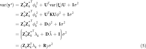is the residual variance. The expectation of y is and the variance is

where and are variance ratios, and .Various methods of inferring a kinship matrix have been proposed. In this study we used a marker-inferred kinship matrix²⁶ defined as

In the single-locus RMLM, the polygenic variance ratio λ is only estimated once under a pure polygenic model (the null model) prior to the marker scanning stage. The estimated variance ratio, , is then treated as a constant when markers are scanned. This approach has been called GWAS with population parameters previously defined (P3D)⁶. The original P3D was implemented when was treated as a fixed effect. In this study, is treated as a random effect, which presents a great challenge in computation. However, we adopted a new algorithm to ease the computation, as described in the following paragraph.

Let us perform eigen decomposition for K so that , where is a diagonal matrix for the eigenvalues and U is an n × n matrix for the eigenvectors. Let , and be transformed variables so that

The expectation of is . The variance-covariance matrix of is

where is a known diagonal matrix. Let 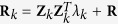be the general covariance structure. After absorbing and σ², we have the following profiled restricted log likelihood function,

where q is the rank of matrix X and

This likelihood function contains only one unknown parameter λ_k. The Newton algorithm for λ_k is

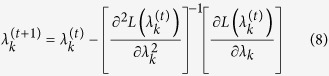Once the iteration process converges, the solution is a single-locus RMLM estimate of λ_k, denoted by . Note that the likelihood function involves and , which are very expensive to compute. However, the special structure of allows us to implement the Woodbury matrix identities²⁷ for calculating and . As a result, the random model approach does not present a substantial increase in computational time.

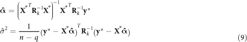
Given , the estimates of and σ² are

The best linear unbiased prediction (BLUP) of γ_k is also the conditional expectation of γ_k given and has the following expression,

The conditional variance is

Under the single-locus RMLM approach, we first estimate and then fix it at to estimate λ_k and scan all markers by testing λ_k = 0 for each SNP. The null hypothesis test for or in the single-locus RMLM is implemented using a Wald test,

The p-value of this Wald test is calculated using

where is a Chi-square variable with one degree of freedom.

Because the estimated marker effects under the random model are shrunken towards zero, we are able to use a modified Bonferroni correction to find the threshold p value for genome-wide significance tests²⁸. This modified Bonferroni correction uses an effective number of markers to adjust for multiple tests so that the threshold p value is , where

is the effective number of markers.

Multi-locus random effect mixed linear model (MRMLM)

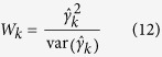
The single marker RMLM method described above can also be considered as an intial screening step for a new multi-locus random effect mixed linear model (MRMLM) that is described here. We use a less stringent criterion for the initial stage screening from RMLM for all markers that have p values smaller than 0.01. In addition, consecutive markers passing the 0.01 threshold around an already selected marker (±20 kb for real data analysis and ± 1 kb for simulated data analysis) are eliminated to reduce collinearity among selected markers. Only these selected markers are included in the muti-locus model for further evaluation, including estimation of marker effects and significane tests. Due to the shrinkage nature, the majority of markers will be eliminated in the intitial screening. Therefore, the number of markers left in the second stage analysis is often a small subset of all markers, say a few hundred or a few thousand at most. Among the remaining markers, all those that passed the modified Bonferroni correction are used to conduct a likelihood ratio test (LRT), and the others are treated as random. If the LOD score for one marker in the LRT is more than 1.50, this marker is treated as fixed, or it is viewed as random. This small number of surviving markers are then included in a single multi-locus model. We propose to use the EM empirical Bayes (EMEB) method¹⁵ because this method also provides a significance test for each marker (likelihood ratio test), while the LASSO method does not have a default method to perform such a test. The EMEB method is also a random model approach because each random marker effect is assigned an empirical distribution with a variance. Because the model is multi-locus in nature, there is no requirement for Bonferroni correction. Therefore, the original 0.05 threshold may be used for significance test. Considering that all markers are selected in the first stage, we decided to place a slightly more stringent criterion of 0.0002, which is converted from LOD score 3.0 of the test statistics using , where is converted from LOD 3 to its corresponding likelihood ratio test, which, under the null hypothesis, follows a Chi-square distribution with one degree of freedom.

Efficient mixed model analysis (EMMA)

This is an existing method for GWAS³ and used as a gold standard for comparison. This method is the fixed model version of the original MLM, in which was treated as a fixed effect with no distribution assigned. The method was implemented in the R software package EMMA ( http://mouse.cs.ucla.edu/emma/). The threshold of p value was set as after Bonferroni correction for multiple tests, where m is the number of markers.

Simulation experiments

In the first four simulation experiments, all the SNP genotypes were derived from the 216130 SNPs in Atwell et al.¹⁶. All the SNPs between 11226256 and 12038776 bp on Chr. 1, between 5045828 and 6412875 bp on Chr. 2, between 1916588 and 3196442 bp on Chr. 3, between 2232796 and 3143893 bp on Chr. 4, and between 19999868 and 21039406 bp on Chr. 5 were used to conduct simulation studies. The sample size was the number of individuals in Atwell et al.¹⁶, namely 199. In the first simulation experiment, six QTNs were simulated and placed on the SNPs with allelic frequencies of 0.30; their heritabilities were set as 0.10, 0.05, 0.05, 0.15, 0.05 and 0.05, respectively; and their positions and effects are listed on Table S1. The average was set at 10.0; and residual variance was set at 10.0. Empirical statistical power for each QTN was calculated as the proportion of samples in which the p value is smaller than the designated threshold p value. A QTN detected within 1 kb of the simulated QTN was considered a true QTN. Empirical Type 1 error for each method was defined as the proportion of significant markers (excluding the markers overlapping with the six QTNs) over all markers with zero effects. In addition to power and Type 1 error, we also evaluated the mean square error (MSE) for each of the six simulated QTNs. For the ith QTN for , the MSE is defined as

where is the estimated effect of QTN i from the jth sample and in the true effect of QTN i. A method with a small MSE is generally more preferable than a method with a large MSE.

To investigate the effect of the polygenic (small effect genes) background on the MRMLM and RMLM methods, the polygenic effect was simulated by multivariate normal distribution , where is the polygenic variance, and is the kinship coefficient matrix between a pair of individuals. Here , so . The QTN size (h²), average, residual variance, and other values were the same as those in the first simulation experiment.

To investigate the effect of epistatic background on the MRMLM and RMLM methods, three epistatic QTNs each with and were simulated. The first one was placed between 3063784 bp on Chr. 4 and 5227063 bp on Chr. 2; the second one was placed between 5986135 bp on Chr. 2 and 2031781 bp on Chr. 3; and the third one was placed between 2668059 bp on Chr. 3 and 11824678 bp on Chr. 1. The QTN sizes (h²), average, residual variance, and other values were also the same as those in the first simulation experiment.

The Arabidopsis thaliana data

We also analyzed the well-known Arabidopsis thaliana data published by Atwell et al.¹⁶. The data contain accessions with genotyped SNPs. Six flowering time related quantitative traits were analyzed using all the three methods (MRMLM, RMLM and EMMA). The six traits are: LD, LDV, SD, 0 W, 2 W and 4 W. These data were downloaded from the following website: http://www.arabidopsis.usc.edu/. We developed our own software to implement the data analysis (see Software S1).

Additional Information

How to cite this article: Wang, S.-B. et al. Improving power and accuracy of genome-wide association studies via a multi-locus mixed linear model methodology. Sci. Rep. 6, 19444; doi: 10.1038/srep19444 (2016).

References

- Zhang Y.M. et al. Mapping quantitative trait loci using naturally occurring genetic variance among commercial inbred lines of maize (Zea mays L.). Genetics 169, 2267– 2275 (2005). [DOI] [PMC free article] [PubMed] [Google Scholar]
- Yu J. et al. A unified mixed-model method for association mapping that accounts for multiple levels of relatedness. Nat. Genet. 38, 203–208 (2006). [DOI] [PubMed] [Google Scholar]
- Kang H.M. et al. Efficient control of population structure in model organism association mapping. Genetics 178, 1709–1723 (2008). [DOI] [PMC free article] [PubMed] [Google Scholar]
- Zhou X. & Stephens M. Genome-wide efficient mixed-model analysis for association studies. Nat. Genet. 44, 821–824 (2012). [DOI] [PMC free article] [PubMed] [Google Scholar]
- Zhou X., Carbonetto P. & Stephens M. Polygenic modeling with Bayesian sparse linear mixed models. PLoS Genet. 9, e1003264 (2013). [DOI] [PMC free article] [PubMed] [Google Scholar]
- Zhang Z. et al. Mixed linear model approach adapted for genome-wide association studies. Nat. Genet. 42, 355–360 (2010). [DOI] [PMC free article] [PubMed] [Google Scholar]
- Li M. et al. Enrichment of statistical power for genome-wide association studies. BMC Biology 12, 73 (2014). [DOI] [PMC free article] [PubMed] [Google Scholar]
- Yi N. & Xu S. Bayesian LASSO for quantitative trait loci mapping. Genetics 179, 1045–1055 (2008). [DOI] [PMC free article] [PubMed] [Google Scholar]
- Hoggart C.J., Whittaker J.C., De Iorio M. & Balding D.J. Simultaneous analysis of all SNPs in genome-wide and re-sequencing association studies. PLoS Genet. 4(7), e1000130 (2008). [DOI] [PMC free article] [PubMed] [Google Scholar]
- Ayers K.L. & Cordell H.J. SNP selection in genome-wide and candidate gene studies via penalized logistic regression. Genetic Epidemiology 34, 879–891 (2010). [DOI] [PMC free article] [PubMed] [Google Scholar]
- Cho S. et al. Joint identification of multiple genetic variants via Elastic-Net variable selection in a genome-wide association analysis. Annals of Human Genetics 74, 416–428 (2010). [DOI] [PubMed] [Google Scholar]
- Lü H.-Y., Liu X.-F., Wei S.-P. & Zhang Y.-M. Epistatic association mapping in homozygous crop cultivars. PLoS ONE 6, e17773 (2011). [DOI] [PMC free article] [PubMed] [Google Scholar]
- Segura V. et al. An efficient multi-locus mixed-model approach for genome-wide association studies in structured populations. Nat. Genet. 44, 825–830 (2012). [DOI] [PMC free article] [PubMed] [Google Scholar]
- Goddard M.E., Wray N.R., Verbyla K. & Visscher P.M. Estimating effects and making predictions from genome-wide marker data. Stat. Sci. 24, 517–529 (2009). [Google Scholar]
- Xu S. An expectation-maximization algorithm for the Lasso estimation of quantitative trait locus effects. Heredity 105, 483–494 (2010). [DOI] [PubMed] [Google Scholar]
- Atwell S. et al. Genome-wide association study of 107 phenotypes in Arabidopsis thaliana inbred lines. Nature 465, 627–631 (2010). [DOI] [PMC free article] [PubMed] [Google Scholar]
- Moser G. et al. Simultaneous discovery, estimation and prediction analysis of complex traits using a Bayesian mixture model. PLoS Genet. 11, e1004969 (2015). [DOI] [PMC free article] [PubMed] [Google Scholar]
- Hartmann U. et al. Molecular cloning of SVP: A negative regulator of the floral transition in Arabidopsis. Plant J. 21(4), 351–360 (2000). [DOI] [PubMed] [Google Scholar]
- Han P., García-Ponce B., Fonseca-Salazar G., Alvarez-Buylla E.R. & Yu H. AGAMOUS-LIKE 17, a novel flowering promoter, acts in a FT-independent photoperiod pathway. Plant J. 55(2), 253–265 (2008). [DOI] [PubMed] [Google Scholar]
- Tominaga R. et al. Arabidopsis CAPRICE-LIKE MYB 3 (CPL3) controls endoreduplication and flowering development in addition to trichome and root hair formation. Development 135, 1335–1345 (2008). [DOI] [PubMed] [Google Scholar]
- Reeves P. & Coupland G. Analysis of flowering time control in Arabidopsis by comparison of double and triple mutants. Plant Physiol. 126, 1085–1091 (2001). [DOI] [PMC free article] [PubMed] [Google Scholar]
- Hepworth S., Valverde F., Ravenscroft D., Mouradov A. & Coupland G. Antagonistic regulation of flowering-time gene SOC1 by CONSTANS and FLC via separate promoter motifs. EMBO J 21, 4327–4337 (2002). [DOI] [PMC free article] [PubMed] [Google Scholar]
- Portolés S. & Más P. Altered oscillator function affects clock resonance and is responsible for the reduced day-length sensitivity of CKB4 overexpressing plants. Plant J. 51(6), 966–977 (2007). [DOI] [PubMed] [Google Scholar]
- Gu X., Wang Y. & He Y. Photoperiodic regulation of flowering time through periodic histone deacetylation of the florigen gene FT. PLoS Biology 11(9), e1001649 (2013). [DOI] [PMC free article] [PubMed] [Google Scholar]
- Hieke S., Binder H., Nieters A. & Schumacher M. minPtest: a resampling based gene region-level testing procedure for genetic case-control studies. Computational Statistics 29(1-2), 51–63 (2014). [Google Scholar]
- Xu S. Mapping quantitative trait loci by controlling polygenic background effects. Genetics 195, 1209–1222 (2013). [DOI] [PMC free article] [PubMed] [Google Scholar]
- Golub G.H. & van Loan C.F. Matrix computations (3rd, Ed) . Baltimore and London: The Johns Hopkins University Press, 1996. [Google Scholar]
- Wang Q., Wei J., Pan Y. & Xu S. An efficient empirical Bayes method for genomewide association studies. J. Anim. Breed. Genet., published online: 19 NOV 2015 10.1111/jbg.12191 (2015). [DOI] [PubMed]
Associated Data
This section collects any data citations, data availability statements, or supplementary materials included in this article.