Comparing the Shape of Contrast Sensitivity Functions for Normal and Low Vision

Abstract

Purpose

The contrast sensitivity function (CSF) provides a detailed description of an individual's spatial-pattern detection capability. We tested the hypothesis that the CSFs of people with low vision differ from a “normal” CSF only in their horizontal and vertical positions along the spatial frequency (SF) and contrast sensitivity (CS) axes.

Methods

Contrast sensitivity for detecting horizontal sinewave gratings was measured with a two temporal-interval forced-choice staircase procedure, for a range of SFs spanning 5 to 6 octaves, for 20 low-vision observers and five adults with normal vision. An asymmetric parabolic function was used to fit the aggregate data of the normal-vision observers, yielding the “normal template.” Each of the 20 low-vision CSFs was fit in two ways, by using a shape-invariant version of the normal template (with the width parameters fixed) that was shifted along the log-SF and log-CS axes, and by an unconstrained asymmetric parabolic function (“free-fit”).

Results

The two fitting methods yielded values of the peak CS, the SF corresponding to peak CS, and the high cut-off SF that were highly correlated and in good agreement with each other. In addition, the width parameters of the low-vision CSFs were comparable with those of the normal template, implying that low-vision CSFs are similar in shape to the normal CSF.

Conclusions

The excellent agreement of parameters estimated by the two fitting methods suggests that low-vision CSFs can be approximated by a normal CSF shifted along the log-SF and log-CS axes to account for the impaired acuity and contrast sensitivity.

Our ability to detect the presence of an object depends on the size of the object (larger is generally easier to detect), and also on the presence of any differences, such as a luminance difference, between the object and its background. The sensitivity to the relative difference in luminance of an object from its background is referred to as contrast sensitivity. Contrast sensitivity depends on object size. A complete representation of how contrast sensitivity depends on object size is referred to as the contrast sensitivity function (CSF), where the object size is usually specified in spatial frequency (c/deg) of a sinewave pattern. As such, the CSF provides a rich description of an individual's spatial-pattern detection capability. Knowing the CSF of a person with low vision is often informative about their ability to see shapes and recognize objects in their daily lives.

The gold standard for determining a CSF is to measure contrast thresholds for detecting sinusoidal gratings across a range of spatial frequencies using robust psychophysical techniques.^1,2 However, this method is time consuming, technically demanding, and requires a carefully calibrated display, and thus is not amenable for the determination of CSF for clinical patients. Recently, a method that uses a Bayesian adaptive procedure to select the spatial frequency and contrast of each trial to maximize the expected information gain has been developed for measuring CSFs.^3,4 The efficiency of this quick CSF method relies on its assumptions about the shape of the CSF and requires 100 trials to achieve good agreement with a CSF measured with the conventional method.⁴ The determination of CSF could be made more efficient if we could reduce the number of measurements required to estimate the full CSF, and link those measurements to standard clinical measures. In fact, an important simplification would exist if low-vision CSFs are similar in shape to normal CSFs, differing only in their positions on the spatial frequency (SF) and contrast sensitivity (CS) axes. In this paper, we test this hypothesis.

There are several ways in which low-vision CSFs could differ in shape from normal-vision CSFs. For example, if contrast sensitivity loss occurs primarily at high spatial frequencies, then the fall-off of contrast sensitivity with high spatial frequencies would be steeper than observed in a normal-vision CSF (Fig. 1A). In the case that contrast sensitivity is equally affected across all spatial frequencies, the resulting CSF would appear as a vertical shift of a normal-vision CSF (Fig. 1B). Alternatively, if the reduction is not uniform across frequencies, then the resulting CSF may look like the one shown in Figure 1C. In addition, notches, representing CS loss only at SFs between the peak SF and the high SF cutoff (Fig. 1D), have been reported for patients with neurologic diseases such as multiple sclerosis.⁵ Notches can also be due to uncorrected refractive errors⁶ or imprecision of measurements⁷; but because they are not the etiologies of low vision, they will not be considered for the purpose of this paper. Despite the fact that some low-vision CSFs may differ in shape from normal-vision CSFs, a previous study (published only in an abstract form) demonstrated that low-vision CSFs were reasonably modeled using a template derived from normally sighted individuals.⁸ In this study, we present empirical evidence showing that indeed, low-vision CSFs can be well described by a normal-vision template appropriately shifted on the SF and CS axes. We focused on measuring CSFs for low-vision observers with visual impairment due to prevalent ocular diseases commonly seen in low-vision clinics.

Figure 1.

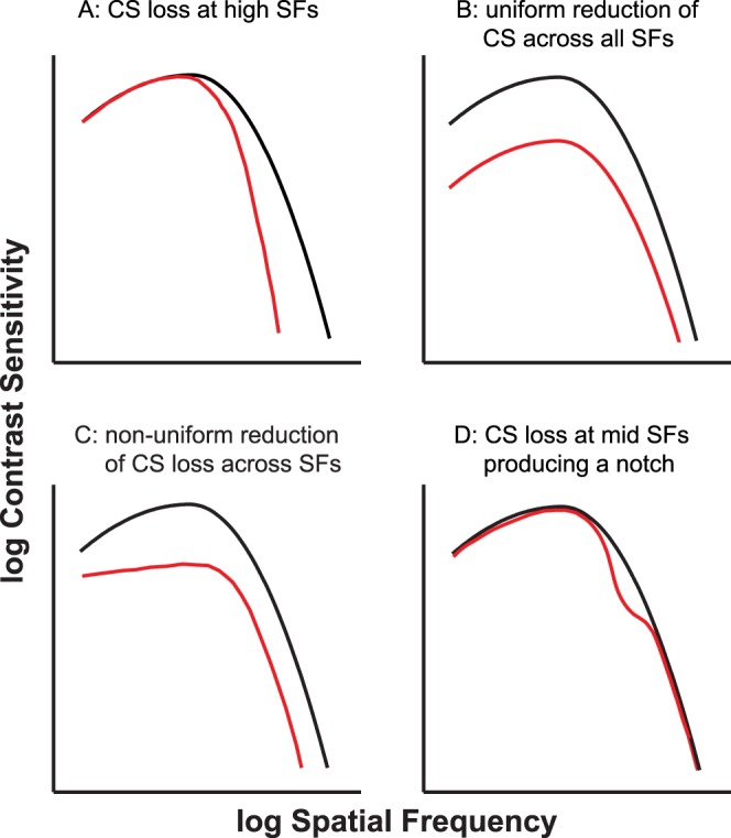
Schematic figure depicting four possibilities for the shape of a low-vision CSF (plotted in red). The black curve in each panel represents the normal-vision CSF. (A) A low-vision CSF that exhibits contrast sensitivity loss only at high spatial frequencies. (B) Uniform CS reduction across all spatial frequencies, resulting in a vertical shift of the normal CSF. (C) An example of a CSF when the CS reduction is not uniform across all spatial frequencies. (D) Contrast sensitivity loss only in the midfrequency range, resulting in a “notch.” This kind of CSF has been reported for patients with neurologic disorders.

Methods

Contrast thresholds for detecting the presence of a sinewave grating with horizontal bars were determined using a two temporal-interval forced-choice paradigm combined with a two-down one-up staircase procedure that tracked performance at 71% accuracy.⁹ Only one spatial frequency was tested in each staircase. The order of frequencies tested was randomized within a session. Grating stimuli were generated using a VSG2/5 video card (Cambridge Research Systems, Rochester, UK) and presented on a SONY 24″ graphics display (model# GDM-FW900; Park Ridge, NJ, USA) at a mean luminance of 75 cd/m². On each trial, a full-field grating with at least five cycles visible, was presented in one of the two temporal intervals that lasted 1 second each with abrupt onset and offset, with a 0.5 second separation between the two intervals. The two temporal intervals were denoted with a high- and low-pitch tone, respectively. Observers indicated the temporal interval in which the grating was presented, guessing if necessary. Feedback on response correctness was not provided. The contrast of the grating decreased by one step following two consecutive trials with correct responses, and increased by one step following a single incorrect response. The step sizes were 0.2 log units for trials before the first two reversals of the staircase and 0.1 log units for subsequent trials. Each staircase terminated after 10 reversals and only the thresholds at the last eight reversals were used for calculating the mean contrast threshold. Each spatial frequency was tested twice, in two different sessions.

Between six and eight spatial frequencies were tested for each low-vision eye. The exact range of spatial frequencies was chosen for each eye such that there were at least two spatial frequencies left of the peak of the CSF and two on the right. For these eyes, the contrast threshold reported for each spatial frequency represents the geometric mean of a total of 16 reversals from two staircases.

To construct the normal template, we tested five normally-sighted observers using the same experimental paradigm with the following changes. First, contrast thresholds were measured for 10 spatial frequencies ranging from 0.4 to 25 c/deg, in steps of 0.2 log units. Second, four staircases were tested for each spatial frequency and each observer, instead of two for low-vision eyes. Thus, at each spatial frequency, the contrast threshold of the normal data represents the geometric mean of 160 staircase reversals (8 reversals per staircase × 4 staircases per observer × 5 observers). These changes were made to ensure precise measurement of the normal template.

Observers

Twenty observers with low vision (12 males and 8 females, mean age = 70.6 ± 11.12 years) and five observers with normal vision (2 males and 3 females, mean age = 25.8 ± 9.9 years) participated in this study. The five observers with normal vision all had best-corrected visual acuity (BCVA) of at least 20/20 in each eye, normal binocular vision and ocular motility function, and no history of any eye diseases. All observers in the low vision group had bilateral vision loss, with a BCVA of 0.14 logMAR (20/25⁻² Snellen equivalent) or worse in the better eye, with a confirmed diagnosis of an eye disease that led to reduced acuity. The diagnoses included AMD, Stargardt disease, glaucoma and optic neuropathy; all of which have been reported to lead to acuity and contrast deficits, and are common etiologies of patients attending low-vision clinics. These observers had a complete low vision evaluation within the 3 months prior to their participation in the study. The Table lists the visual characteristics of the low-vision observers. All observers, normal or low vision, gave informed oral and written consent before the commencement of data collection. The research followed the tenets of the Declaration of Helsinki and was approved by the institutional review board at the first author's institution. All observers were tested monocularly, with the nontested eye covered using a standard black-cloth eye-patch. Low-vision observers were tested using the eye with the better acuity. Normal-vision observers were tested using their left eyes.

Table.

Visual Characteristics of the 20 Eyes With Low Vision

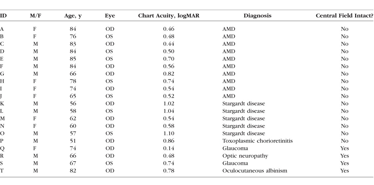
We chose to use young adults, instead of age-matched older adults, for constructing the normal-vision template mainly for two reasons. Most importantly, our hypothesis of a shift of the normal template to account for acuity and contrast deficits is not age-specific. Second, because of our need to construct a high-quality normal template, it was more practical to test young, normally-sighted adults on the more rigorous and time-consuming CSF data collection.

Curve-Fitting and Statistical Analyses

Although many functions have been used to describe normal CSFs (see Watson and Ahumada¹⁰ for a comparison of the different functions), we adopted an asymmetric parabolic function, which is simple to construct, and provides an excellent fit to our normal-vision data. The function, which requires four parameters, is given by the following equation:

where f(SF) is the contrast sensitivity at a spatial frequency SF, CS_p is the peak contrast sensitivity, SF_p is the spatial frequency at which CS_p occurs, and width_L and width_R are the curvatures of the left and right branches of the asymmetric parabolic function, respectively. The values for contrast sensitivity and spatial frequency were log-transformed before curve-fitting. Curve-fitting was performed using Igor Pro (WaveMetrics, Inc., Lake Oswego, OR, USA), which uses a Levenberg-Marquardt iterative algorithm (a form of nonlinear least-squares fitting) to minimize the χ² error between the experimental and the model fit.

To evaluate whether the shapes of the low-vision CSFs were the same as that of the normal-vision CSF, we first constructed a “normal template” by determining the four parameter values yielding the best-fit function to the normal-vision data using Equation 1. Then we compared two fitting methods, free-fit versus template-fit, for each low-vision CSF. Free-fit was accomplished by fitting a low-vision CSF using Equation 1 and allowing all four parameters to vary. Template-fit also made use of Equation 1 but with the two parameters, width_L and width_R, constrained to the values returned for the best-fit function for the normal-vision data. The template fit allowed only variation in the peak contrast sensitivity CS_p and the spatial-frequency at the peak SF_p. The effect of this restriction is to retain the shape of the CSF while permitting only translation of the function horizontally and vertically along the log spatial frequency and log contrast sensitivity axes. Model comparisons of the four- and two-parameter fits for the low-vision CSFs were performed using the Akaike Information Criterion¹¹ (AIC), which takes into account the goodness-of-fit of each fitting method, given the number of free parameters used. According to Akaike, the model with the smaller overall AIC value is the model of choice.¹¹

Besides comparing the goodness-of-fit, we also compared several key parameters of the fitted functions derived from the two fitting methods, to determine how well these parameters correlate or agree with each other. The degree of agreement was examined using the Bland-Altman analysis.¹² If the shape of low-vision CSFs is the same as that for the normal-vision CSF, then the normal template should fit the low-vision data just as well as the free-fit. The goodness-of-fit of the two fitting methods would be similar, and that the key parameters derived from the two methods would show a strong correlation and agreement with each other. All statistical analyses reported in this article were performed using the R software.¹³

Results

We will first present the CSF data of the normal vision observers, to be used in constructing the “normal template.” Then we will compare the fitting of the normal template and the free-fit to the CSFs of the low vision observers. Key parameters derived from the template fit and the free-fit will also be compared.

Figure 2 shows the contrast sensitivity versus spatial frequency data of our group of normal vision observers. Each data point represents the contrast sensitivity, the reciprocal of the geometric mean of contrast thresholds across the five normal vision observers, with 32 staircase reversals for each observer (eight reversals per staircase and four staircases per observer). Error bars represent the SD of the mean sensitivity based on 1000 bootstrap resamplings. To derive the “normal-vision CSF,” we fit the data set using the asymmetric parabolic function (Equation 1). The best-fit function returns the following parameters: peak contrast sensitivity, CS_p = 2.22 log units (corresponds to 166); spatial frequency at which peak contrast sensitivity occurs, SF_p = 0.4 log c/deg (corresponds to 2.5 c/deg); width_L = 0.68 and width_R = 1.28. This normal-vision CSF (solid line through the data points in Fig. 2), with the width parameters constrained to the values of the best-fit curve, forms our normal template.

Figure 2.

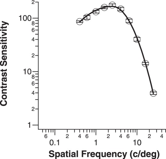
Contrast sensitivity is plotted as a function of spatial frequency (c/deg) for the five normal-vision control observers. Each data point represents the sensitivity (reciprocal of contrast threshold) based on eight reversals per staircase, four staircases per observer, and five observers. Error bars represent the SD of the mean sensitivity based on 1000 bootstrap resamplings.

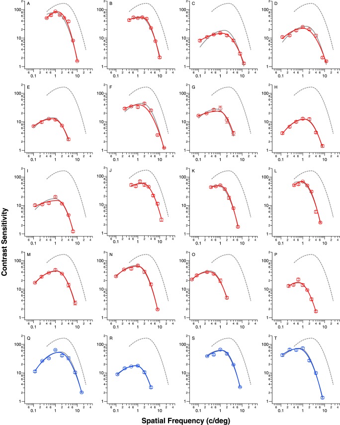
Data of the low-vision observers are shown in Figure 3. These data are color-coded: red for those with central field loss and blue for those with intact central field. We categorized the low-vision observers in this way because the presence or absence of central field loss is often associated with substantial differences in reading and other real-world activities. Each low-vision observer's CSF data were fit separately using the two fitting methods, the best-fit curve using the free-fit method is given in each panel in the same color as the symbols and the best-fit curve using the template-fit is given as the gray solid line.

Figure 3.

Contrast sensitivity is plotted as a function of spatial frequency (c/deg) for the 20 eyes with low vision. Data are color-coded: red for observers with central field loss and blue for observers with intact central field. Each data point represents the sensitivity (reciprocal of contrast threshold) based on 16 reversals (8 reversals per staircase for 2 staircases). Error bars represent the SD of the mean sensitivity based on 1000 bootstrap resamplings. The best-fit curves according to the free-fit and template-fit are given as the color (red or blue) and gray solid curves, respectively. The normal-vision CSF is also given in each panel as the gray dashed curve.

We first evaluated which of the two fitting methods provided a better description of individual low-vision CSFs. To do so, we compared the sum of the AIC of the two fitting methods across all low-vision eyes, with AIC given by

where k is the number of free parameters (4 for free-fit and 2 for template-fit). The method with the smaller sum of AIC is the better model.¹¹ Using this method, the sum of AIC is 231.2 for the free-fit method and 231.1 for the template-fit, implying that the two fitting methods provide equally good fits to the low-vision data.

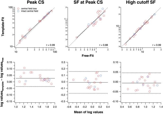
We examined the correlation and agreement of three key parameters derived from the two fitting methods, the peak contrast sensitivity (CS_p), the spatial frequency at peak contrast sensitivity (SF_p), and the high cutoff spatial frequency. CS_p and SF_p are parameters returned by the two fitting methods, while the high cutoff spatial frequency was derived from Equation 1, by setting f(SF) to a value of 1 and solving for the corresponding spatial frequency. The top panels in Figure 4 show how well each of these parameters derived from the two fitting methods correlate with each other. A t-test on the correlation coefficients (r ranging from 0.88–0.99) shows that all of these correlations are statistically significant (P < 0.0001), indicating that the parameters from the two fitting methods correlate strongly with each other. Because high correlation does not necessarily mean good numerical agreement, we also examined the data in Bland-Altman plots¹² (bottom panels in Fig. 4) to determine how well each of these parameters derived from the two fitting methods agree with each other. We reason that if the ±95% limits of agreement (plotted as dashed lines in each of the bottom panels) are comparable with the test–retest reliability of similar measurements, then the two fitting methods are in good agreement with each other. The 95% limits of agreement for CS_p are ±0.06 log units, which are smaller than the published data on test-retest reliability of contrast sensitivity measurement using the Pelli-Robson Chart¹⁴ or the MARS Chart,¹⁵ with values ranging from ±0.15 to ±0.33 log units.^16–18 For SF_p, the 95% limits of agreement are ±0.17 log units, but because we know of no published data on the test-retest reliability of SF_p, or of similar measurement, we cannot compare our measurements with previous data. The 95% limits of agreement for the high cutoff spatial frequency are ±0.05 log units, smaller than the test-retest reliability of visual acuity measurement (equivalent to the high cutoff spatial frequency), which ranges between ±0.1 and ±0.2 log units.^19,20 Thus, in general, the parameters derived from the two fitting methods are in good agreement.

Figure 4.

Values derived from the free-fit and template-fit methods are compared for the peak contrast sensitivity (CS_p), the spatial frequency that yields the peak contrast sensitivity (SF_p) and the high cutoff spatial frequency. In the top panels, we examine how well these values from the two fitting methods correlate with each other. Data are color-coded, and the black line in each panel represents the best-fit regression line. The gray dashed line in each panel represents the 1:1 line. In the bottom panels, we examine, in the form of Bland-Altman plots, how well the values between the two fitting methods agree with each other. The black solid and dashed lines in each panel represent the mean of the difference of log values between the two fitting methods and the 95% limits of agreement, respectively.

Note that the main results do not change if we consider only data for eyes with central field loss. The correlation coefficients for the values estimated for the two fitting methods remain unchanged (0.99 for CS_p, 0.88 for SF_p, and 0.99 for the high cutoff spatial frequency), and remain statistically significant (P < 0.0001). In addition, Bland-Altman plots show that the values derived from the two fitting methods still agree well with each other. These additional analyses ensure that our conclusion that the free-fit method provides a good fit to the low-vision CSF data is still valid if we consider only patients with central field loss.

Given our hypothesis of low-vision CSFs having the same shape as the normal CSF, it is important to compare the parameters that govern the shape of the fitted functions. These are the width_L and width_R parameters. In Figure 5, we represent the distributions of the width_L and width_R parameters for the low-vision CSFs, derived from the free-fit method in box-and-whisker plots. The gray dashed lines show the values of these parameters for the normal template. A test for normality based on the Shapiro-Wilk test showed that the distribution for width_L does not follow a normal distribution (W = 0.89, P = 0.03) but the distribution for width_R is not different from a normal distribution (W = 0.94, P = 0.28). Therefore, we used the Mann-Whitney U test to evaluate whether these distributions, derived from the free-fit method, are different from the parameter values for the normal CSF. While values for the parameter width_R do not differ between the free-fit method and the constrained value (U = 200, P = 1.0), values for width_L are different between the free-fit method and the constrained value (U = 100, P = 0.004). Indeed, Figure 3 shows that for several data-sets, the free-fit method yields a fitted curve with a shallower low-frequency decline than that returned by the template fit, especially for eyes C, D, F, G, and I. However, the means of the two distributions, represented by the red circles, are very close to the constrained values.

Figure 5.

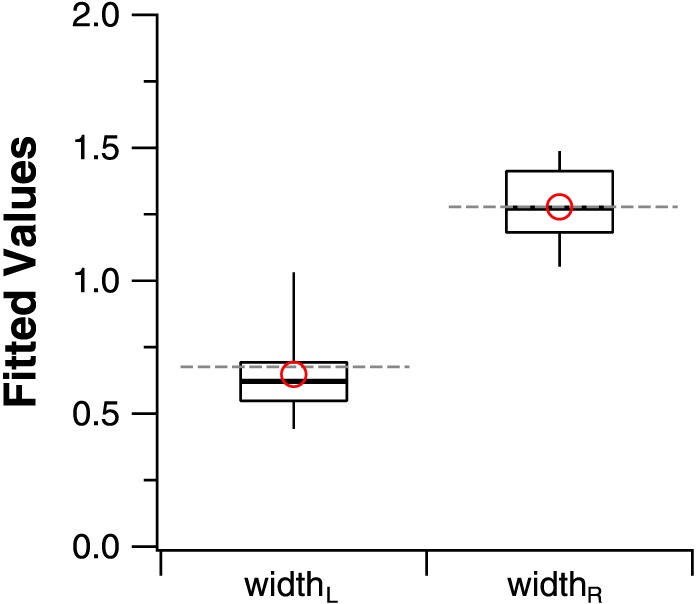
Box-and-whisker plots comparing the values of width_L and width_R derived from the free-fit method with the constrained values based on the normal CSF. The upper and lower bound of each box represent the 75th and 25th percentiles of the distribution, and the median is represented by the thick line within the box. The top and bottom ends of the whisker represent the 95th and 5th percentiles of the distribution, respectively. Red circles represent the means of the two distributions. Note that the mean values are very similar to the parameter values for the normal template, shown as gray dashed lines.

Results from these analyses show that the free-fit method provides a description of the low-vision CSF data that is very similar to the template-fit, which is derived from the normal-vision data. We acknowledge that some of the low-vision CSFs are more low-pass in shape, resulting in the sample distribution of the parameter width_L being different from that of the constrained value, however, the mean of the sample distribution (0.64) is very similar to that of the constrained value (0.68).

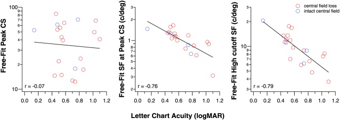
Considering that the template fit only has two free parameters, our results suggest that low-vision CSFs can be related to a normal CSF with two additional measurements. A practical question is whether letter-chart acuity, a clinical measurement performed on every clinical patient, can be one of the two additional measurements. Here, we seek to determine if letter-chart acuity can predict some of the key parameters of the fitted CSF functions. To do so, we examined if there exists a significant correlation between letter-chart acuity, measured using a Bailey-Lovie Chart²¹ with acuity expressed in logMAR, and each of the three key parameters: CS_p, SF_p, and the high cutoff spatial frequency, as derived from the free-fit method. As shown in Figure 6, the correlation between CS_p and acuity is weak (r = −0.07; P = 0.78), but there is a high correlation between SF_p and acuity (r = −0.76; P < 0.0001), and between the high cutoff spatial frequency and acuity (r = −0.79; P < 0.0001). In other words, letter-chart acuity can explain 58% and 62% of the variances in SF_p and the high cutoff spatial frequency.

Figure 6.

The correlation between CS_p (left), SF_p (middle), and the high cutoff SF (right) with letter-chart acuity.

Once again, when we consider only data for eyes with central field loss, the results remain practically the same. The correlation between CS_p and acuity remains weak and insignificant (r = 0.05; P = 0.84), while the correlations remain high between SF_p and acuity (r = −0.76; P = 0.0006), and between the high cutoff spatial frequency and acuity (r = −0.75; P = 0.0009).

The high cutoff spatial frequency of the CSF represents the smallest detail that can be resolved, thus theoretically it should agree well with letter-chart acuity. The Bland-Altman plot in Figure 7 shows how well the high cutoff spatial frequency derived from the free-fit method agrees with the letter-chart acuity. The high cutoff spatial frequencies were converted to their equivalent logMAR acuities by assuming that individual bars of the sinewave grating are the spatial details to be resolved. As an example, the critical feature of a 20/20 letter (logMAR 0.0) subtends 1 arc min, and each light and dark bar of a 30 c/deg grating subtends 1 arc min. Therefore, a cutoff spatial frequency of 30 c/deg is often taken to correspond to a letter acuity of 20/20. This method essentially assumes that the letter frequency for identification is 2.5 c/letter, although the critical frequency for letter identification may vary depending on conditions such as letter size, retinal eccentricity, and so on.^22,23 The ±95% limits of agreement are ±0.28 log units, larger than the test-retest reliability of visual acuity measurement of ±0.1 to 0.2 log units.^19,20 In addition, the mean acuity difference between the high cutoff spatial frequency and chart acuity is 0.15 logMAR, which is statistically different from a null difference (P = 0.0002). These results show that in general, using the conversion that 20/20 letters correspond to 30 c/deg, the letter-chart yields a poorer acuity than the high cutoff spatial frequency. Therefore, attempts to derive the full CSF using the letter-chart acuity as one of the two measurements need to take into account this constant difference.

Figure 7.

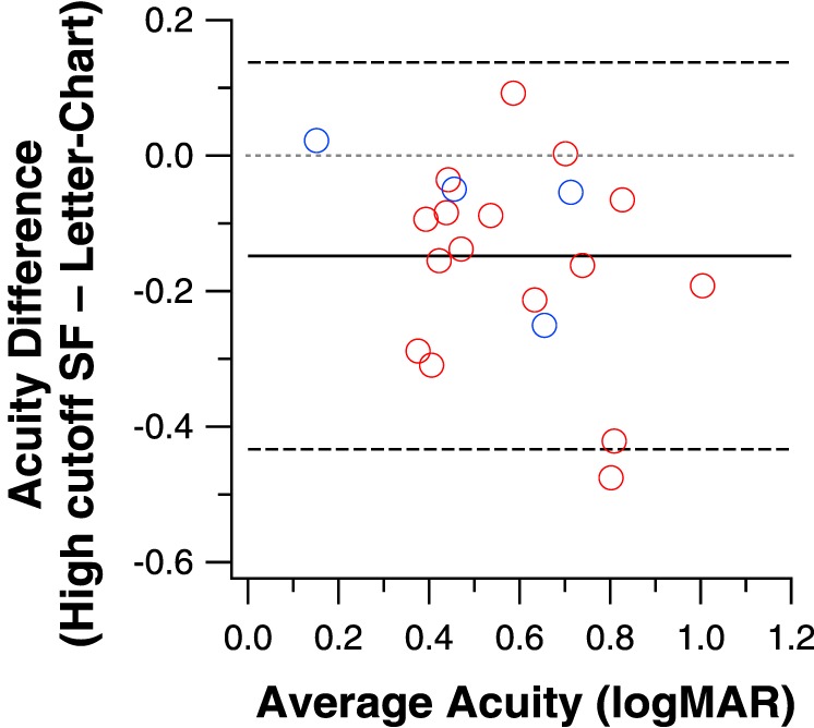
Letter-chart acuity and the high cutoff spatial frequency derived from the free-fit method (converted to logMAR acuity) are compared in a Bland-Altman plot. The mean difference between the two methods is 0.15 logMAR (black solid line) and is statistically different from 0 (gray dotted line).

Discussion

Contrast sensitivities and visual acuities are affected in many ocular diseases that lead to impaired vision, thus leading to many reports that the CSFs of individuals with diseases such as macular disorders,^24–27 glaucoma,^28,29 and optic neuropathy³⁰ are different from that of a “normal” CSF. To our knowledge, Pelli et al.⁸ was the first investigation to test the hypothesis that low-vision CSFs have the same shape as that of a normal-vision CSF. They measured the CSFs of 32 low-vision observers and fit each set of log CS versus log SF data using a single parabola that was derived from four normally sighted observers. By constraining the shape of the parabolic template but allowing it to shift vertically and horizontally along the log CS and log SF axes, Pelli et al.⁸ found that the parabolic template provided a good fit to all the low-vision CSFs. Subsequently, Rohaly and Owsley³¹ applied the method of Pelli et al.⁸ and fit a parabolic function to the data of 100 older adults aged between 53 and 85 years, with an average acuity of 20/25; and found that the parabolic template did not provide a good fit for 20% of their observers. These authors also attempted to fit their data using an exponential function³² but again found that the function did not provide a good fit to their data. This led the authors to conclude that the CSFs of older adults could not be described by a single parabolic or exponential function with two or three free parameters. Differences in the observer characteristics (low vision versus older adults with relatively good vision) aside, there are several key methodologic differences between our study and that of Rohaly and Owsley.³¹ Rohaly and Owsley³¹ had their observers adjust the contrast of a grating stimulus until they just detected the grating (method of adjustment). We used a two temporal interval forced-choice paradigm combined with a staircase procedure. It is well known that a criterion-free forced-choice method usually provides more reliable measurements of contrast threshold than the method of adjustment.^33,34 This might account for why the shapes of the CSFs for some of their observers were unusual, as shown in their paper. Most noticeably, in several figures in their paper, contrast sensitivities were practically invariant for a large range of low- to high-spatial frequencies, and the contrast sensitivity at the highest-spatial frequency (22.5 c/deg) was still much higher than expected (based on published data). This unusual trend of contrast sensitivity data, and the lack of a clear fall-off of sensitivity at high-spatial frequencies make it difficult for any function with a high-frequency roll-off to provide a good fit. It was indeed because of this reason that we tested a range of spatial frequencies that included at least two frequencies lower than, and at least two frequencies higher than the peak of the CSF.

More recently, Watson and Ahumada¹⁰ compared 11 functions to describe a large set of CSF data obtained from normally sighted observers using a variety of stimuli (the ModelFest data), and found that many of the functions fit the data similarly well. Most of these functions contain four free parameters. These authors cautioned the use of a template that is based on a set of average data in fitting an individual observer's data. Nevertheless, in our study, we found that a template based on the average data of a group of normally-sighted observers provides a reasonably good fit to individual data of 20 low-vision eyes. The close coupling between the low- and normal-vision CSFs does not even require the normal-vision template to be derived from age-matched control observers. Presumably, shifting the normal template to fit the low-vision data accounts for the visual deficits of the individual, regardless of whether the deficits are due to ocular diseases or normal aging. Had we found that the shifted normal template did not provide a good fit to the low-vision data, the age difference between our young normal and low-vision groups would have been a possible factor accounting for the difference, and that the use of a normal template derived from normally sighted observers age-matched with those of the low-vision group would have been necessary.

It is well known that the rates of fall-off of contrast sensitivity with spatial frequency differ for the left and right branches of the CSF with respect to CS_p, thus in this study, we chose an asymmetric parabolic function to fit our data because it allows for different rates of fall-off (or the width parameters in Equation 1) for the left and right branches of the CSF. An asymmetric parabolic function has four free parameters. By constraining two of these parameters that determine the shape (width) of the function, our template only contains two free parameters. Recently, Pelli and Bex³⁵ suggested that a template with four free parameters, as in the many models evaluated by Watson and Ahumada,¹⁰ might provide a better fit to individual data. Here, we showed that a model with only two free parameters might be sufficient, and in fact, the template fit with only two free parameters yielded an overall AIC value that is virtually identical to that of the free-fit with four free parameters.

A practical advantage of modeling CSFs with a template that requires only two free parameters is that we only need two measurements in addition to the template to derive a full CSF, thus offering an efficient method for the determination of the CSF. If our concern is to obtain an estimate of the CSF of a patient with low vision, then one of these two measurements could be the conventional acuity measurement, since acuity is measured for every patient in the clinic, and that letter chart acuity correlates strongly with both the spatial frequency at the peak of the CSF and the high cutoff spatial frequency (Fig. 6). As for the second measurement, there are many clinical tests of contrast sensitivity, such as the Bailey-Lovie Low Contrast Acuity Chart³⁶ or Regan Charts,³⁷ which measure acuity for letters at a fixed low contrast; the Pelli-Robson Chart¹⁴ or the MARS Chart,¹⁵ which provide a contrast sensitivity measurement close to the peak of the CSF; and other contrast sensitivity tests such as the Melbourne Edge Test,³⁸ and the Berkeley Discs Contrast Sensitivity test (Bailey IL, et al. IOVS 2011;52:E-Abstract 1892). The differences in acuity and a clinical contrast sensitivity measurement between a low-vision individual and the norms could then be used to shift a normal CSF horizontally along the log SF axis and vertically along the log CS axis. As an example, assume a low-vision individual had an acuity of 0.4 logMAR and a contrast sensitivity as measured using the Pelli-Robson Chart of 1.35 log units. Now, let us further assume that the normal values for acuity and contrast sensitivity measurements using the same charts are −0.1 logMAR and 2.1 log units; then the differences in acuity and contrast sensitivity between the low-vision individual and normals become 0.5 and 0.75 log units, respectively. In this case, the CSF of the low-vision individual can be approximated by shifting a normal CSF template leftward along the log SF axis by 0.5 log units to account for the difference in acuity, and downward along the log CS axis by 0.75 log units to account for the difference in contrast sensitivity. Whether or not our conjecture of using just two clinical measurements, visual acuity and contrast sensitivity, can yield a full CSF closely resembles that measured using the “gold standard” (using grating stimuli) would need to be empirically validated in future studies.

Two caveats should be kept in mind when interpreting our results. First, the specific shape of a CSF is stimulus-dependent and may change with stimulus parameters such as luminance,³⁹ retinal eccentricity,⁴⁰ field size,^41,42 duration,⁴³ and the temporal characteristics of the gratings.^44,45 For example, the shape of a CSF changes from band-pass to low-pass with a reduction in the mean luminance of the gratings from photopic to scotopic level, an increase in retinal eccentricity, a briefer presentation of the grating stimulus or when there is an increased temporal modulation. The close coupling between the low- and normal-vision CSFs observed in this study applies to the set of stimulus conditions used in this study. Given that our set of stimulus parameters is fairly generic, it is likely that the close coupling is quite general and would apply to measurements made with other stimulus parameters. Nevertheless, future investigations may wish to establish their own normal template to ensure the best fitting of their low-vision data, especially if these investigations are going to use stimulus parameters drastically different from those used in this study. Second, although our group of low-vision observers includes etiologies of ocular disease commonly seen in low-vision clinics, it did not include patients with cataracts or neurologic disorders such as multiple sclerosis. Patients with cataracts whose disability is more due to glare may show a selective reduction in contrast sensitivity at low spatial frequencies. Multiple sclerosis, although infrequently seen in low-vision clinics, has been shown to produce notches in the CSF in the midfrequencies,⁵ which could make it difficult for any function to provide a good description of the CSF. It remains to be verified whether or not a normal template, ours or others, can be used to fit the CSF of these conditions, or other conditions that lead to the shape of the CSF being different from that of the normal template.

An efficient method of determining a full CSF is useful for individuals with normal vision, but it is especially useful for low vision as the peak contrast sensitivity is a good predictor of daily activities such as mobility,⁴⁶ face recognition,⁴⁷ and reading.⁴⁸ In the laboratory, full low-vision CSFs can be used as filters to recreate visual stimuli that simulate what individuals with low vision can detect. This may be a useful tool for informal evaluation of the impact of vision impairment, especially acuity loss and reduced contrast sensitivity, on visibility of real-world objects and scenes. In the clinic, filtering visual scenes using the CSF of a low-vision patient may help family members understand what the patient can see or why there are difficulties with certain tasks. It should be recognized, however, that using the CSF as a linear filter has significant limitations in simulating low-vision visibility. More sophisticated models of feature visibility, such as that of Peli,⁴⁹ may include multiple spatial-frequency channels and the ability to represent local luminance-dependent variations in contrast sensitivity across the visual field.

In this study, we have learned that the contrast sensitivity functions (CSFs) of many low-vision subjects have the same shape as the CSFs of normally-sighted subjects, but differ from the normal CSFs in two values, the spatial frequency and contrast sensitivity at the peak of the curve. These two values are closely associated with clinical measures of acuity and contrast sensitivity. This means that by coupling our knowledge of the characteristic CSF curves of normally-sighted subjects with two readily available clinical measures from a patient with low vision, we can infer a rich and informative description of the patient's pattern vision.

References

- 1. Schade OH. Optical and photoelectric analog of the eye. J Opt Soc Am. 1956; 46: 721–739. [DOI] [PubMed] [Google Scholar]
- 2. Campbell FW,, Robson JG. Application of Fourier analysis to the visibility of gratings. J Physiol. 1968; 197: 551–566. [DOI] [PMC free article] [PubMed] [Google Scholar]
- 3. Lesmes LA,, Jeon ST,, Lu ZL,, Dosher BA. Bayesian adaptive estimation of threshold versus contrast external noise functions: the quick TvC method. Vision Res. 2006; 46: 3160–3176. [DOI] [PubMed] [Google Scholar]
- 4. Lesmes LA,, Lu ZL,, Baek J,, Albright TD. Bayesian adaptive estimation of the contrast sensitivity function: the quick CSF method. J Vis. 2010; 10 (3): 17.1–17.21. [DOI] [PMC free article] [PubMed] [Google Scholar]
- 5. Regan D,, Silver R,, Murray TJ. Visual acuity and contrast sensitivity in multiple sclerosis—hidden visual loss: an auxiliary diagnostic test. Brain. 1977; 100: 563–579. [DOI] [PubMed] [Google Scholar]
- 6. Campbell FW,, Green DF. Optical and retinal factors affecting visual resolution. J Physiol. 1965; 181: 576–593. [DOI] [PMC free article] [PubMed] [Google Scholar]
- 7. Rubin GS. Reliability and sensitivity of clinical contrast sensitivity tests. Clin Vision Sci. 1988; 2: 169–177. [Google Scholar]
- 8. Pelli DG,, Rubin GS,, Legge GE. Predicting the contrast sensitivity of low-vision observers. J Opt Soc Am A. 1986; 3: 56. [Google Scholar]
- 9. Wetherill GB,, Levitt H. Sequential estimation of points on a psychometric function. Br J Math Stat Psychol. 1965; 18: 1–10. [DOI] [PubMed] [Google Scholar]
- 10. Watson AB,, Ahumada AJ,, Jr. A standard model for foveal detection of spatial contrast. J Vis. 2005; 5 (9): 717–740. [DOI] [PubMed] [Google Scholar]
- 11. Akaike H. A new look at the statistical model identification. IEEE Trans Auto Control. 1974; AC-19:716–723.
- 12. Bland JM,, Altman DG. Statistical methods for assessing agreement between two methods of clinical measurement. Lancet. 1986; 1: 307–310. [PubMed] [Google Scholar]
- 13. R Development Core Team. R: A language and environment for statistical computing. Vienna, Austria: R Foundation for Statistical Computing; 2014. Available at: http://www.R-project.org/. Accessed July 2015. [Google Scholar]
- 14. Pelli DG,, Robson JG,, Wilkins AJ. The design of a new letter chart for measuring contrast sensitivity. Clin Vis Sci. 1988; 2: 187–199. [Google Scholar]
- 15. Arditi A. Improving the design of the letter contrast sensitivity test. Invest Ophthalmol Vis Sci. 2005; 46: 2225–2229. [DOI] [PubMed] [Google Scholar]
- 16. Elliott DB,, Sanderson K,, Conkey A. The reliability of the Pelli-Robson contrast sensitivity chart. Ophthalmic Physiol Opt. 1990; 10: 21–24. [PubMed] [Google Scholar]
- 17. Dougherty BE,, Flom RE,, Bullimore MA. An evaluation of the Mars Letter Contrast Sensitivity Test. Optom Vis Sci. 2005; 82: 970–975. [DOI] [PubMed] [Google Scholar]
- 18. Haymes SA,, Roberts KF,, Cruess AF,, et al. The letter contrast sensitivity test: clinical evaluation of a new design. Invest Ophthalmol Vis Sci. 2006; 47: 2739–2745. [DOI] [PubMed] [Google Scholar]
- 19. Arditi A,, Cagenello R. On the statistical reliability of letter-chart visual acuity measurements. Invest Ophthalmol Vis Sci. 1993; 34: 120–129. [PubMed] [Google Scholar]
- 20. Kiser AK,, Mladenovich D,, Eshraghi F,, Bourdeau D,, Dagnelie G. Reliability and consistency of visual acuity and contrast sensitivity measures in advanced eye disease. Optom Vis Sci. 2005; 82: 946–954. [DOI] [PubMed] [Google Scholar]
- 21. Bailey IL,, Lovie JE. New design principles for visual acuity letter charts. Am J Optom Physiol Opt. 1976; 53: 740–745. [DOI] [PubMed] [Google Scholar]
- 22. Chung STL,, Legge GE,, Tjan BS. Spatial-frequency characteristics of letter identification in central and peripheral vision. Vision Res. 2002; 42: 2137–2152. [DOI] [PubMed] [Google Scholar]
- 23. Majaj NJ,, Pelli DG,, Kurshan P,, Palomares M. The role of spatial frequency channels in letter identification. Vision Res. 2002; 42: 1165–1184. [DOI] [PubMed] [Google Scholar]
- 24. Wolkstein M,, Atkin A,, Bodis-Wollner I. Contrast sensitivity in retinal disease. Ophthalmology. 1980; 87: 1140–1149. [DOI] [PubMed] [Google Scholar]
- 25. Marmor MF. Contrast sensitivity versus visual acuity in retinal disease. Br J Ophthalmol. 1986; 70: 553–559. [DOI] [PMC free article] [PubMed] [Google Scholar]
- 26. Sunness JS,, Rubin GS,, Applegate CA,, et al. Visual function abnormalities and prognosis in eyes with age-related geographic atrophy of the macula and good visual acuity. Ophthalmology. 1997; 104: 1677–1691. [DOI] [PMC free article] [PubMed] [Google Scholar]
- 27. Mei M,, Leat SJ. Suprathreshold contrast matching in maculopathy. Invest Ophthalmol Vis Sci. 2007; 48: 3419–3424. [DOI] [PubMed] [Google Scholar]
- 28. Stamper RL. The effect of glaucoma on central visual function. Trans Am Ophthalmol Soc. 1984; 82: 792–826. [PMC free article] [PubMed] [Google Scholar]
- 29. Ross JE,, Bron AJ,, Clarke DD. Contrast sensitivity and visual disability in chronic simple glaucoma. Br J Ophthalmol. 1984; 68: 821–827. [DOI] [PMC free article] [PubMed] [Google Scholar]
- 30. Beck RW,, Ruchman MC,, Savino PJ,, Schatz NJ. Contrast sensitivity measurements in acute and resolved optic neuritis. Br J Ophthalmol. 1984; 68: 756–759. [DOI] [PMC free article] [PubMed] [Google Scholar]
- 31. Rohaly AM,, Owsley C. Modeling the contrast-sensitivity functions of older adults. J Opt Soc Am A. 1993; 10: 1591–1599. [DOI] [PubMed] [Google Scholar]
- 32. Kelly DH. Spatial frequency selectivity in the retina. Vision Res. 1975; 15: 665–672. [DOI] [PubMed] [Google Scholar]
- 33. Kelly DH,, Savoie RE. A study of sine-wave contrast sensitivity by two psychophysical methods. Percept Psychophys. 1973; 14: 313–318. [Google Scholar]
- 34. Higgins KE,, Jaffe MJ,, Caruso RC,, deMonasterio FM. Spatial contrast sensitivity: effects of age, test-retest, and psychophysical method. J Opt Soc Am A. 1988; 5: 2173–2180. [DOI] [PubMed] [Google Scholar]
- 35. Pelli DG,, Bex P. Measuring contrast sensitivity. Vision Res. 2013; 90: 10–14. [DOI] [PMC free article] [PubMed] [Google Scholar]
- 36. Bailey IL. New procedures for detecting early vision losses in the elderly. Optom Vis Sci. 1993; 70: 299–305. [DOI] [PubMed] [Google Scholar]
- 37. Regan D,, Neima D. Low-contrast letter charts as a test of visual function. Ophthalmology. 1983; 90: 1192–1200. [DOI] [PubMed] [Google Scholar]
- 38. Verbaken JH,, Johnston AW. Clinical contrast sensitivity testing; the current status. Clin Exp Optom. 1986; 69: 205–212. [Google Scholar]
- 39. De Valois RL,, Morgan H,, Snodderly DM. Psychophysical studies of monkey vision. 3. Spatial luminance contrast sensitivity tests of macaque and human observers. Vision Res. 1974; 14: 75–81. [DOI] [PubMed] [Google Scholar]
- 40. Rovamo J,, Virsu V,, Nasanen R. Cortical magnification factor predicts the photopic contrast sensitivity of peripheral vision. Nature. 1978; 271: 54–56. [DOI] [PubMed] [Google Scholar]
- 41. Savoy RL,, McCann JJ. Visibility of low-spatial-frequency sine-wave targets: dependence on number of cycles. J Opt Soc Am. 1975; 65: 343–350. [DOI] [PubMed] [Google Scholar]
- 42. Rovamo J,, Luntinen O,, Nasanen R. Modelling the dependence of contrast sensitivity on grating area and spatial frequency. Vision Res. 1993; 33: 2773–2788. [DOI] [PubMed] [Google Scholar]
- 43. Legge GE. Sustained and transient mechanisms in human vision: temporal and spatial properties. Vision Res. 1978; 18: 69–81. [DOI] [PubMed] [Google Scholar]
- 44. Robson JG. Spatial and temporal contrast-sensitivity functions of the visual system. J Opt Soc Am. 1966; 56: 1141–1142. [Google Scholar]
- 45. Kelly DH. Motion and vision. II. Stabilized spatio-temporal threshold surface. J Opt Soc Am. 1979; 69: 1340–1349. [DOI] [PubMed] [Google Scholar]
- 46. Marron JA,, Bailey IL. Visual factors and orientation mobility performance. Am J Optom Physiol Opt. 1982; 59: 413–426. [DOI] [PubMed] [Google Scholar]
- 47. Wolffsohn JS,, Eperjesi F,, Napper G. Evaluation of Melbourne Edge Test contrast sensitivity measures in the visually impaired. Ophthalmic Physiol Opt. 2005; 25: 371–374. [DOI] [PubMed] [Google Scholar]
- 48. Rubin GS,, Legge GE. Psychophysics of reading. VI – the role of contrast in low vision. Vision Res. 1989; 29: 79–91. [DOI] [PubMed] [Google Scholar]
- 49. Peli E. Contrast in complex images. J Opt Soc Am A. 1990; 7: 2032–2040. [DOI] [PubMed] [Google Scholar]