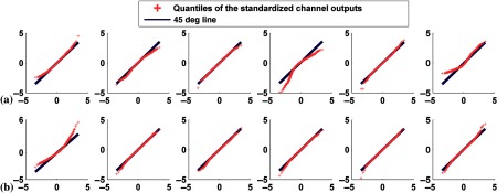
Abstract.
The channelized Hotelling observer (CHO) uses the first- and second-order statistics of channel outputs under both hypotheses to compute test statistics used in binary classification tasks. If these input data deviate from a multivariate normal (MVN) distribution, the classification performance will be suboptimal compared to an ideal observer operating on the same channel outputs. We conducted a comprehensive investigation to rigorously study the validity of the MVN assumption under various kinds of background and signal variability in a realistic population of phantoms. The study was performed in the context of myocardial perfusion SPECT imaging; anatomical, uptake (intensity), and signal variability were simulated. Quantitative measures and graphical approaches applied to the outputs of each channel were used to investigate the amount and type of deviation from normality. For some types of background and signal variations, the channel outputs, under both hypotheses, were non-normal (i.e., skewed or multimodal). This indicates that, for realistic medical images in cases where there is signal or background variability, the normality of the channel outputs should be evaluated before applying a CHO. Finally, the different degrees of departure from normality of the various channels are explained in terms of violations of the central limit theorem.
Keywords: model observers, channelized Hotelling observer, image quality
1. Introduction
Objective evaluation of medical imaging systems and algorithms is essential for progress in medical imaging. In this context, classification tasks, and especially binary classification (detection) tasks, are important and clinically relevant.1,2
Mathematical model observers have found an important place in the objective evaluation of medical images since they are better predictors of human observer performance than the traditional measures of image quality such as image resolution, variance, contrast, or mean square error.1 The ideal observer (IO) and the Hotelling observer (HO) are examples of widely used model observers. In a binary classification task, the IO requires the full knowledge of the probability density functions (PDFs) of the input data under both hypotheses. Determining these PDFs is challenging when the input data are realistic medical images from a patient population. The HO is a linear classifier and can thus be used as an alternative to the IO, requiring only the knowledge of the first- and second-order statistics of the image data.1–7 It is the optimal linear discriminant and has performance equal to the IO under certain conditions (see below). Due to its simplicity, the HO has been extensively used in medical imaging to assess image quality.1–4 However, the HO tends to outperform the human observer in the presence of correlated noise.8 Thus, the channelized Hotelling observer (CHO) has been proposed, where a frequency-selective channel mechanism is often applied to more closely approximate the performance of the IO9,10 or the human observer,11–14 depending on the choice of the channel model. In addition, the use of a small number of channels reduces the dimensionality of the observer.1 Several studies have shown that the CHO, with an appropriate channel model, can successfully predict human observer performance in the case of signal known exactly and background known exactly (SKE/BKE) detection task using simulated images11 and using realistic single-photon emission computed tomography (SPECT) images.14 Moreover, the CHO is a good predictor of the human observer in the case of signal known exactly and background known statistically (SKE/BKS) tasks.15,16 The signal known statistically and background known statistically (SKS/BKS) task poses limits to the CHO methodology as discussed in Park et al.9,16,17 An example of SKS tasks is presented in Ref. 1, where Barrett and Myers discussed the effect of signal variability on the HO performance and presented an example of signal location variability, showing that the data from the defect-present class can follow a non-normal distribution as well as multimodal patterns. They have also proposed the concept of model observers for a signal known exactly but variable (SKEV) task to approximate performance in the SKS tasks. This concept has been further discussed by Eckstein et al.18,19
For a binary classification task, the performance of the HO is the same as that of the IO if the input data from both classes have multivariate normal (MVN) PDFs with equal covariance matrices.1,7 To provide a better understanding of the behavior of different observers, Park et al.9,16 studied the effect of image statistics on the performance of the CHO and the human observer as compared to the IO. Park et al.9 found that the CHO was suboptimal (i.e., it gave a smaller area under the receiver operating characteristics curve) compared to the IO if the images were non-normally distributed. Park et al.16 found that, in the case of an SKE task, the human efficiency (relative to the IO) for normally distributed lumpy backgrounds (LBs) was much higher than that for non-normally distributed LBs.
The CHO is the HO applied to the channel outputs. If the channel outputs under both hypotheses do not follow MVN distributions, then the performance of the CHO will be suboptimal compared to (i.e., not the same as) the IO applied to the channel outputs. Since the channel outputs are the weighted sums of multiple random variables (i.e., image pixel values), it is often assumed that the channel outputs are MVN because of the central limit theorem (CLT).1,20 The classical CLT states that the arithmetic mean of a large number of independent and identically distributed random variables approaches a normal distribution. The basic assumptions of the CLT can be relaxed to various degrees resulting in different versions of CLT with different degrees of generality.21–23 The degree to which these assumptions are relaxed affects how well the mean of the random variables approximates a normal distribution.20,24–26
The normality of channel outputs is commonly assumed in the literature where, to the best of our knowledge, no formal investigation has been conducted nor reported to quantify the deviation from normality of the channel outputs for various background and signal variabilities. Since data from clinical studies of human populations include these variabilities, it is desirable to be able to handle these variations in model observers, and thus to facilitate the use of model observers in the evaluation and optimization of imaging systems and processing methods for human patient populations. As demonstrated in this paper, these kinds of variations challenge the MVN assumption, indicating the need for caution when applying CHO methods directly to image data with this kind of variation. Knowledge of the factors affecting the distribution of the channel outputs could help in the formulation of model observers and methods in cases where such background and signal variability are present, as will be discussed in Sec. 5.3.
We carried out this study in the context of myocardial perfusion SPECT (MPS) imaging, where the task is to detect the presence of perfusion defects in SPECT images of the myocardium. However, the analysis and principles developed in this work are applicable to other imaging modalities and organs of interest. Background variations are an important factor limiting task performance in clinical studies for many medical imaging modalities and applications. These variations arise from variability in patient anatomy and, in nuclear medicine, from uptake in organs of interest. Thus, we investigated the effects of background variations, including anatomical and organ uptake variability, and signal variability, including variation in perfusion defect extent (size), severity (contrast), and location. The images used in this study were postprocessed using low-pass filtering and, except where noted, nonlinear windowing, and discretization to mimic the procedures used in display of clinical images.27–32
The MVN assumption was examined using a set of quantitative and qualitative measures of normality applied to the outputs of each channel. In the discussion section, we address the normality results in the context of the CLT in an effort to provide insight into cases where one can expect the channel outputs to be non-MVN. We studied how well the data satisfied the main requirements of the CLT and investigated how the relaxation of these requirements affected the distribution of the channel outputs.
2. Channelized Hotelling Observer Methodology
A brief explanation of the CHO methodology is provided in this section. A full explanation of the HO and CHO can be found in Ref. 1. In a binary detection task with single defect detection, the goal of the observer is to separate two classes of images: the defect-absent class and the defect-present class. The images consist of a background, with or without a signal, and are corrupted by noise. In the context of this work, the signal is a perfusion defect (i.e., a region with reduced uptake in the myocardium) in an MPS scan; the background consists of the activity in the various tissues of the body (including the myocardium) surrounding the defect. The shape, size, position, and uptake (image intensity) of these background tissues can vary.
We denote the defect-absent and the defect-present hypotheses as and , respectively. Consider an imaging system where the acquired image vector under the ’th hypothesis for , 2 is denoted by the -dimensional vector . For a binary detection task, the SNR is a common measure of class separability for a certain observer. The SNR is defined by
| (1) |
where and are the ensemble mean and the variance of the outputs of the observer for hypothesis , respectively. The outputs of the observer are known as the test statistics. The HO is a linear observer that uses the first and second moments of the image data under both hypotheses and maximizes the SNR. The Hotelling template is a linear operator applied to the image data to produce the test statistic. The Hotelling template is given by
| (2) |
where are the ensemble mean vectors of the image data from the ’th class, and is the intraclass scatter matrix defined as
| (3) |
where are the covariance matrices of the image data from the ’th class. Under both hypotheses, the test statistic for the HO is a scalar quantity, and it is given by
| (4) |
The calculation of the Hotelling template requires the inversion of , which is computationally challenging due to its huge size (in our work, is a matrix). Thus, a frequency-selective channel mechanism is often applied to reduce the dimensionality of the observer, as well as to better model the performance of human observer or IO. Let be the channel matrix in the spatial domain, where is the number of channels used (usually ). By applying the channel model, we take the product of the -element image vector and the channel matrix in the spatial domain.27 This is equivalent to taking the dot product of and each of the spatial domain channels. This results in an -element feature vector (i.e., channel output) under each hypothesis denoted by . Then, for each class of images, we have
| (5) |
The CHO is the HO applied to the channelized data. Thus, the CHO is the linear observer that maximizes the SNR computed using the channel outputs. The CHO template is given by
| (6) |
where are the ensemble mean vectors of the channel outputs of the ’th class, and is the intraclass scatter matrix computed from the channel outputs. Under both hypotheses, the test statistic for the CHO is given by
| (7) |
From Eq. (6), the template for the CHO is calculated using the mean vector and the intraclass covariance matrix of the channelized data. If the channel outputs are not MVN, the performance of the CHO will be suboptimal as compared to IO applied to the same channel outputs.
3. Methods
3.1. Phantom Population and Projection Data
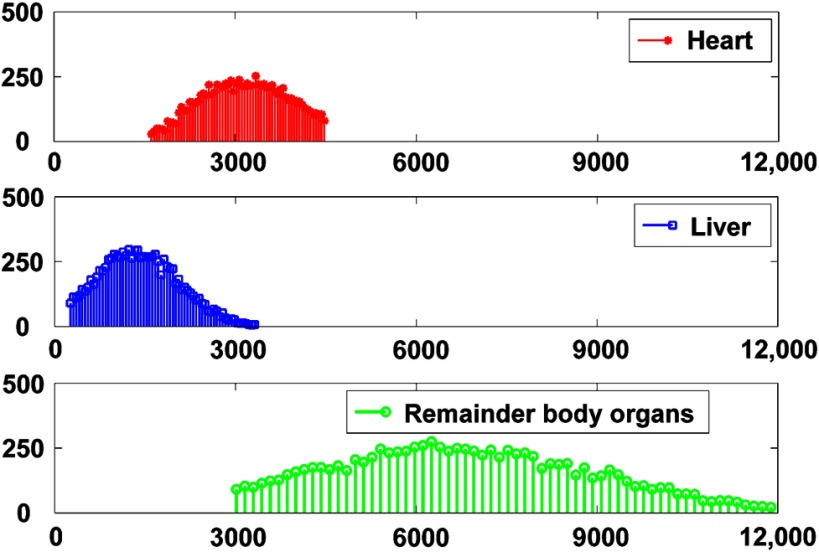
The phantom population used in this study has been previously described in Ghaly et al.33 The following is a brief overview. Projection data of the three-dimensional (3-D) extended cardiac-torso (XCAT) phantom34,35 were generated using an analytical projector that modeled attenuation, scatter, full collimator detector response including septal penetration and scatter, and Pb x-ray generation of a GE low-energy and high-resolution collimator, a 9.5-mm-thick NaI(Tl) crystal with an energy resolution of 9% and a 4-mm full-width at half-maximum intrinsic spatial resolution. Projection images were generated in a matrix with a pixel size of 0.442 cm and simulated at 60 equally spaced angles over a 180-deg acquisition arc extending from 45 deg right anterior oblique to 45 deg left posterior oblique. We modeled 10 mCi of Tc-99m labeled agents. The data were generated to model MPS imaging using a conventional SPECT system. The population included 54 anatomical variations corresponding to two genders and three variations (small, medium, and large) each of body size, heart size, and subcutaneous adipose tissue thickness. The range of sizes used was based on the distribution of sizes in a sample of clinical images. The uptake variability in organs was based on quantitative analysis of clinical studies and was modeled by sampling from truncated normal distributions for the relevant organs as shown in Fig. 1.33 In the dataset used here, separate projection datasets were generated for the heart, liver, and remainder of the body organs. The individual projections were scaled based on these sampled activity values to account for uptake variability.
Fig. 1.
Sixty-four bin histogram plots of the reconstructed counts per unit volume (counts/cm3) in the different organs.
In MPS imaging, signal variability results from variations in location, severity, and extent. To this end, we simulated defects at two different locations in the myocardial wall. Both defects were midventricular: one was in the anterolateral wall and the other in the inferior wall. For each location, we generated defects with three severities: 10%, 25%, and 50%. In MPS imaging, defect severity is defined as the percentage reduction in tracer uptake (activity concentration) in the defect relative to the normal myocardium. The severities investigated are clinically significant and range from mild to moderate, and thus provide a range of difficulty in defect detection. Finally, for each location and severity we studied two defect extents: 5% and 25%. The defect’s extent is defined as the percentage of myocardial volume occupied by the perfusion defect. These extents represent small and large perfusion defect sizes, respectively.
3.2. Image Reconstruction and Postreconstruction Processing
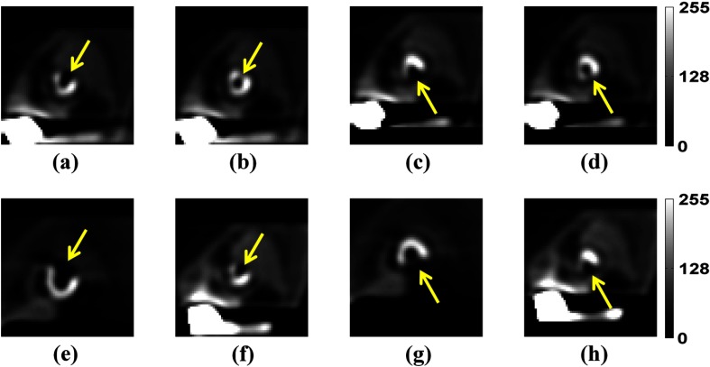
SPECT images were reconstructed from the simulated projections using filtered backprojection (FBP). The reconstructed images had cubic voxels with a side length of 0.442 cm. The reconstructed images were postprocessed to generate short-axis images analogous to those viewed clinically as described in Refs. 27, 32, and 36. This postprocessing includes low-pass filtering, reorientation to short axis (involving interpolation), intensity windowing, and discretization. First, the reconstructed transaxial images were filtered with a 3-D Butterworth filter with order eight and cutoff frequencies 0.08, 0.16, or to provide various levels of noise control. These cutoff frequencies spanned a range that included optimal frequencies for MPS images reconstructed using iterative reconstruction methods.13,27,32 Next, the filtered images were reoriented into a short-axis orientation, where the images were sliced perpendicular to the long axis of the left ventricle. Next, a image centered on the position of the small defect for the defect-present class or the corresponding defect location for the defect-absent class was extracted and windowed. The windowing and discretization steps are nonlinear steps as they include truncation, scaling, and rounding.27–32 In the truncation step, negative values were mapped to zero. Next, in the scaling step, any pixel value that was larger than or equal to the maximum pixel value in the heart was mapped to 255 and values between zero and the maximum were mapped to the range [0, 255]. Finally, the resulting floating-point values were rounded to integer values. These nonlinear steps mimic the procedures used in display of clinical images.27–32 A sample of the resulting images for different phantom anatomies and defects is shown in Fig. 2.
Fig. 2.
The images are noise-free short-axis postprocessed images for different defects and phantoms. The arrows indicate the defects’ position, which were generated with a severity of 100% to aid visualization. The images shown in (a)–(d) are from the male phantom with the smallest value for all three anatomical parameters. Images (a) and (b) show anterolateral defects with extents of 25% and 5%, respectively. Images (c) and (d) show inferior defects with extents of 25% and 5%, respectively. The images shown in (e) and (f) have an anterolateral defect with an extent of 25%, where (e) is from the male phantom with the largest value for all three anatomical parameters and (f) is from the female phantom with the smallest value for all three anatomical parameters. The images shown in (g) and (h) have an inferior defect with an extent of 25%, where (g) is from the male phantom with the largest value for all three anatomical parameters and (h) is from the female phantom with the smallest value for all three anatomical parameters.
3.3. Application of the Frequency-Selective Channel Model
We used six rotationally symmetric frequency channels (RSC) denoted by , which are octave-wide, bandpass filters with a square profile, as described in Ref. 11 and given mathematically by
| (8) |
where and is the starting frequency of the first channel.
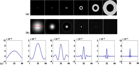
The first channel had a starting frequency and width both equal to . Subsequent channels were adjacent, nonoverlapping, and had double the width of the previous channel. The frequency channels and corresponding spatial domain channels are shown in Fig. 3. Similar channel models have commonly been used in the evaluation and optimization of nuclear medicine instrumentation design, acquisition parameters, and reconstruction parameters.12,27,37 Also, they have been used for analysis of myocardial perfusion images and have resulted in good predictions of the rankings of human observers.12 The two-dimensional (2-D) frequency domain channels were transformed analytically to the spatial domain and then sampled. To mimic the human visual system, the DC component was explicitly set to zero by subtracting the mean of the spatial channel. The channels were applied to the postprocessed images described earlier by taking the dot product of the image and each of the spatial domain channels as discussed in Sec. 2. This process resulted in a six-element channel output (feature) vector for each input image.
Fig. 3.
The six channels used in this work. The leftmost column represents the lowest frequency channel (channel 1). The channel’s start frequency and width increase from left to right. The rows are (a) the frequency domain channels, (b) the spatial domain channels, and (c) the horizontal profiles through the origin of the spatial channels as indicated by the line in the leftmost image in (b), where the horizontal axis is the pixel number and the vertical axis is the pixel value.
3.4. Assessment of the Multivariate Normality Assumption of the Channel Outputs
The MVN of a distribution may be tested using an MVN test such as the Henze test.38,39 This tests the hypothesis that all the channel outputs are MVN. However, this does not provide much insight into the source of the MVN violation. Another way of MVN testing is to use a set of univariate normality (UVN) tests with the null hypothesis that the individual channel outputs are normally distributed as suggested in Refs. 40–42. The normality of each channel is a necessary, but not sufficient, condition for the data to be MVN.40,42 The one-sample Kolmogorov–Smirnov (K–S)43 or Pearson’s Chi-square44 are common UVN tests.
However, one problem with hypothesis testing is that it does not communicate the type and size of departure from normality. Thus, to evaluate quantitatively the degree of departure from normality, we computed the correlation coefficient between the quantiles of the individual channel outputs and the quantiles of a standard normal distribution:45 the closer the correlation coefficient is to 1, the stronger the linear relation between the two distributions. Other measures of the deviation from normality were the skewness and kurtosis.42 We calculated these quantities for the individual channel outputs and compared them to those expected for a normal distribution, which has a skewness of zero and kurtosis of 3.
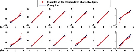
Nevertheless, the aforementioned quantitative measures often do not detect the presence of a multimodal distribution. Thus, we used a qualitative (graphical) approach to provide visual confirmation of the degree of non-normality of the individual channel outputs and to detect the presence of multimodal distributions. We used plots of both the histograms and the quantile–quantile (Q–Q) plots42,46 for this purpose. The histograms are easy to understand, but the shape of the histogram depends on the number of bins used. Thus, we also used Q–Q plots, which are more robust to factors such as the number of bins. In a Q–Q plot, the quantiles of the standardized distribution (obtained by subtracting the mean from the data and then dividing by the standard deviation) of the outputs from each channel are plotted against the quantiles of the standard normal distribution. If the points on this plot are not close to the 45 deg line, this indicates a departure from normality.
4. Results
The following presents the results of a set of numerical experiments investigating the distribution of the channel outputs when different types and combinations of background and signal variations were present. In this work, the signal was known to the observer in the sense that the center of the spatial domain channels was the same as the center of the defect for the defect-present images or the corresponding location for the defect-absent images. However, the extent and the severity varied, in some cases, from one image to another. Unless noted, a cutoff frequency of was used. Also, channels were numbered from 1 to 6 in order of increasing start frequency, i.e., from left to right as shown in Fig. 3.
4.1. No Signal Variability and No Anatomical Variability
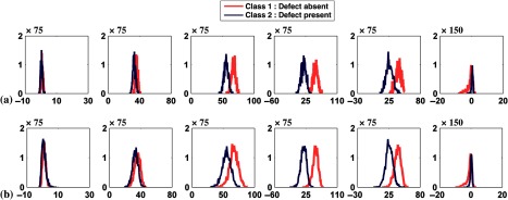
We started with the case when neither signal variability nor anatomical variability was present using the male phantom with small heart size, body size, and subcutaneous adipose tissue thickness and the anterolateral defect with extent and severity both equal to 25%. We investigated the case of with and without organ uptake varaiblity. We generated 2000 pairs of defect-absent and defect-present images. The histograms and the Q–Q plots of channel outputs with and without uptake variability are shown in Figs. 4 and 5, respectively. When uptake variability was modeled, the widths of the histograms were wider than when uptake variability was not modeled. The results, shown in Fig. 4, indicate that, for both classes, the widths (standard deviations) increased by a factor of almost 2 for the first three channels and almost 1.2 for the fourth and fifth channels. For the sixth channel, this factor was and ~1.3 for the defect-absent and the defect-present classes, respectively. Thus, this factor was not uniform across the channels. This increase in the widths of the histograms is expected because uptake variability results in a varying number of counts in the different organs individually and the image as a whole, thus producing a larger range of outputs for each channel.
Fig. 4.
Histogram plots of the channel outputs when neither signal nor anatomical variability was included. The horizontal axis is the channel output intensity and the vertical axis is the frequency of occurrence. The columns represent the outputs from the six channels as defined in Fig. 3. The rows are (a) without uptake variability and (b) with uptake variability. Sixty-four histogram bins were used.
Fig. 5.
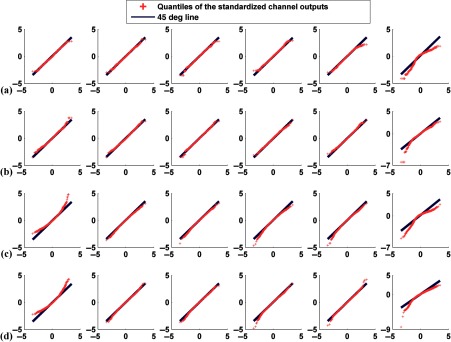
Q–Q plots comparing the distributions of standardized channel outputs and the theoretical standard normal distribution when neither signal nor anatomical variability was included. The horizontal axis represents the quantiles of standard normal distribution; the vertical axis is the quantiles of the standardized channel outputs. The columns represent the outputs from the six channels defined in Fig. 3. Rows (a) and (b) are without uptake variability, where plots in (a) represent defect-absent and (b) defect-present data. Rows (c) and (d) are with uptake variability, where plots in (c) represent defect-absent and (d) defect-present data.
Tables 1 and 2 report the correlation coefficient, , and skewness, and kurtosis values calculated from each individual channel outputs without and with uptake variability, respectively. From Fig. 5 and Tables 1 and 2 observe that uptake variability affected the degree of non-normality of the channel outputs. For example, with uptake variability the output from channel 1 was more positively skewed (e.g., for the defect-absent class, the skewness values were 0.07 and 0.93 without and with uptake variability, respectively). This observation was true for both the defect-absent and defect-present classes. Furthermore, the histogram of channel 6 was more skewed toward the left and more peaked for both classes when uptake variability was included. This is consistent with observations from the Q–Q plots.
Table 1.
Results of correlation coefficienta (), skewness, and kurtosis values for the channel outputs without uptake, anatomical or signal variability.
| Channel number | |||||||
|---|---|---|---|---|---|---|---|
| 1 | 2 | 3 | 4 | 5 | 6 | ||
| Defect absent | 1.00 | 1.00 | 1.00 | 1.00 | 0.99 | 0.93 | |
| Defect present | 1.00 | 1.00 | 1.00 | 1.00 | 1.00 | 0.97 | |
| Kurtosis | Defect absent | 2.79 | 2.83 | 2.98 | 2.91 | 2.59 | 4.68 |
| Defect present | 2.91 | 2.94 | 3.09 | 2.69 | 2.99 | 6.72 | |
| Skewness | Defect absent | 0.07 | 0.02 | 0.07 | |||
| Defect present | 0.22 | 0.21 | 0.02 | 0.21 | |||
The values have been rounded to two decimal places.
Table 2.
As Table 1, for the case of uptake variability, without anatomical or signal variability.
| Channel number | |||||||
|---|---|---|---|---|---|---|---|
| 1 | 2 | 3 | 4 | 5 | 6 | ||
| Defect absent | 0.98 | 1.00 | 1.00 | 0.99 | 0.99 | 0.93 | |
| Defect present | 0.97 | 1.00 | 1.00 | 1.00 | 1.00 | 0.95 | |
| Kurtosis | Defect absent | 5.04 | 3.05 | 3.31 | 3.66 | 3.61 | 5.79 |
| Defect present | 5.01 | 3.35 | 3.36 | 3.65 | 3.66 | 7.69 | |
| Skewness | Defect absent | 0.93 | |||||
| Defect present | 1.00 | 0.00 | |||||
4.2. Anatomical Variability and No Signal Variability
This experiment evaluated the addition of different levels of anatomical variability in the presence of uptake variability without signal variability. The same defect was used as in Sec. 4.1.
4.2.1. Mixture of two phantoms
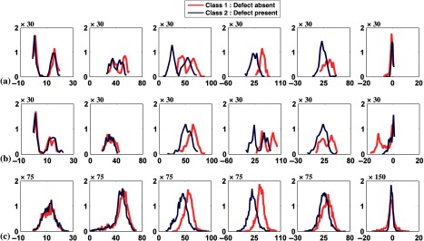
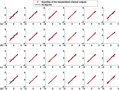
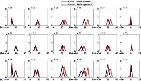
First, we investigated two different anatomies. For each phantom, we generated 100 uptake realizations of noisy projection data for each class, resulting in 200 pairs of defect-absent and defect-present images. In the first experiment, we considered the case of two male phantoms with different sizes. In particular, we used phantoms having the smallest and largest values of all three anatomical parameters (see Fig. 2). In the second experiment, we investigated the effect of gender variation using the phantoms for each gender having the smallest values of the three anatomical parameters (see Fig. 2). For both experiments, when the channel outputs from the two phantoms were pooled, the distribution of the channel outputs was bimodal for some of the channels for both classes as indicated in Figs. 6(a), 6(b), and 7.
Fig. 6.
Histogram plots of the channel outputs with anatomical variability and without signal variability. The axes are as described in Fig. 4. The columns represent the outputs from the six channels defined in Fig. 3. The rows are histogram plots for the cases of (a) the two male phantoms with different sizes, (b) two different genders, and (c) all 54 phantoms. The histograms in rows (a) and (b) used 16 bins while those in row (c) used 64 due to the larger number of feature vectors.
Fig. 7.
Q–Q plots comparing the distributions of standardized channel outputs with the theoretical standard normal distribution with anatomical variability and without signal variability. The axes are as described in Fig. 5. The columns represent the outputs from the six channels defined in Fig. 3. Rows (a) and (b) are for the case of the two male phantoms with different sizes, where plots in (a) represent defect-absent and (b) defect-present data. Rows (c) and (d) are for the case of the two phantoms with different genders, where plots in (c) represent defect-absent and (d) defect-present data.
4.2.2. Mixture of all 54 phantoms
For each of the 54 phantom anatomies, we generated 37 uptake realizations of noisy projection data for each class, resulting in 1998 pairs of defect-absent and defect-present images. When the channel outputs from all 54 different phantoms were pooled, the histograms of the channel outputs were unimodal as shown in Figs. 6(c) and 8. By comparing Figs. 4(b) and 6(c), we observed that the widths of the histograms were wider in the case of 54 anatomical variations than when no anatomical variation was present. The correlation coefficient values, skewness, and kurtosis are reported in Table 3.
Fig. 8.
As Fig. 7 for the case of 54 phantoms, where plots in (a) represent defect-absent and (b) defect-present data.
Table 3.
As Table 1, for the case of anatomical variability (54 phantoms) without signal variability.
| Channel number | |||||||
|---|---|---|---|---|---|---|---|
| 1 | 2 | 3 | 4 | 5 | 6 | ||
| Defect absent | 1.00 | 0.95 | 0.99 | 0.99 | 1.00 | 0.97 | |
| Defect present | 1.00 | 0.95 | 0.99 | 1.00 | 1.00 | 0.94 | |
| Kurtosis | Defect absent | 2.51 | 4.98 | 4.18 | 4.69 | 3.28 | 5.78 |
| Defect present | 2.89 | 5.51 | 3.81 | 3.92 | 3.87 | 11.69 | |
| Skewness | Defect absent | 0.19 | 0.07 | ||||
| Defect present | 0.05 | 0.17 | 0.16 | ||||
4.3. Signal Variability and No Anatomical Variability
In this experiment, different types of signal variations were studied for a single phantom (male with the smallest value for all three anatomical parameters) with uptake variability. We investigated the individual effects of variability in location, extent, and severity.
4.3.1. Variation of defect location
In this experiment, we used both the anterolateral and inferior defect locations with extents and severities both equal to 25%. For each defect location 1000 noisy images were generated, resulting in 2000 pairs of defect-absent and defect-present images. Figures 9(a) and 9(b) show the histogram plots of the channel outputs for the individual defect location; Fig. 9(c) shows the histogram when channel outputs for both locations were pooled. In Fig. 9(c) observe that the distributions of the channel outputs were bimodal for channels 1, 2, and 4 for both the defect-absent and defect-present classes.
Fig. 9.
Histogram plots of the channel outputs with signal location variability and without anatomical variability. The extent and severity of the defects were both equal to 25%. The axes are as described in Fig. 4. The columns represent the outputs from the six channels defined in Fig. 3. The rows are from (a) the anterolateral, (b) inferior, and (c) the mixture of anterolateral and inferior defects. Sixty-four histogram bins were used.
4.3.2. Variation in defect severity
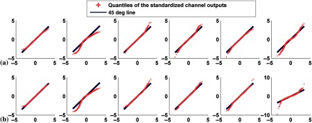
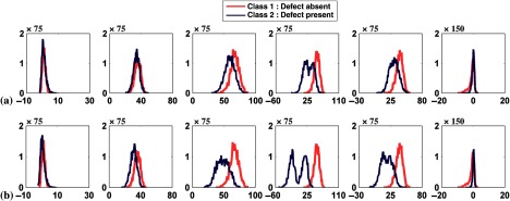
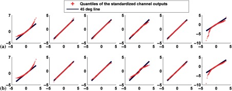
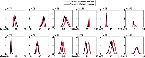
For this experiment, we investigated the effect of varying the defect severity for a fixed location (anterolateral) and extent (25%). We studied two combinations of defect severities: [10%, 25%] and [25%, 50%], respectively. For each defect severity, 1000 images were generated, resulting in 2000 pairs of defect-absent and defect-present images. We observed that the histograms of the channel outputs for pooled data were bimodal for some channels for the defect-present class, as shown in Figs. 10 and 11. For example, the two modes of the histogram from channel 4 were more separated for the combination of the 25% and 50% severity defects. The histograms of the channel outputs for the defect-absent class were unimodal for all channels.
Fig. 10.
Histogram plots of the channel outputs with signal severity variability and without anatomical variability. The extent of the defects was 25% and they were located in the anterolateral wall. The axes are as described in Fig. 4. The columns represent the outputs from the six channels defined in Fig. 3. The rows are from (a) the mixture of defect severities of 10% and 25% and (b) 25% and 50%. Sixty-four histogram bins were used.
Fig. 11.
Q–Q plots comparing the distributions of standardized channel outputs with the theoretical standard normal distribution with signal severity variability and without anatomical variabilities. The extent of the defects was 25% and they were located in the anterolateral wall. The axes are as described in Fig. 5. The columns represent the outputs from the six channels defined in Fig. 3. The rows are for defect-present data, having a mixture of defect severities of (a) 10% and 25% and (b) 25% and 50%.
4.3.3. Variation in defect extent
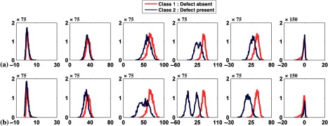
Finally, we investigated the case of variations in defect extent for the anterolateral defect. We combined defects with extents of 5% and 25% for both 25% and 50% severities. For each severity, we generated 1000 images for each defect extent, resulting in 2000 pairs of defect-absent and defect-present images. As shown in Figs. 12 and 13, the distributions of the channel outputs were unimodal for the defect-absent class. However, for the defect-present class, the distribution was bimodal for channel 4 and the separation between the two modes increased with defect severity.
Fig. 12.
Histogram plots of the channel outputs with signal extent variability and without anatomical variability. The defects’ extents were 5% and 25%. They were located at the anterolateral wall. The axes are as described in Fig. 4. The columns represent the outputs from the six channels defined in Fig. 3. The rows represent the (a) 25% and (b) 50% severity cases. Sixty-four histogram bins were used.
Fig. 13.
Q–Q plots comparing the distributions of standardized channel outputs with the theoretical standard normal distribution with signal extent variability and without anatomical variability. The defects’ extents were 5% and 25%. They were located at the anterolateral wall. The axes are as described in Fig. 5. The columns represent the outputs from the six channels defined in Fig. 3. The rows are for the defect-present data having severities of (a) 25% and (b) 50%.
5. Discussion
The data presented in the aforementioned experiments demonstrated that, for the set of realistic medical images used, the MVN assumption of the channel outputs did not hold when some kinds of background and signal variability were present. For the simple case—when neither uptake nor anatomical nor signal variability was present and the only source of randomness was due to quantum noise—the distributions of individual channel outputs were close to normal, except for the highest frequency channel. When uptake variability was introduced, the distribution of individual channel outputs started to deviate from normality.
In the case of a limited number of background or signal variations, the distribution of the channel outputs was bimodal for some channels and unimodal for others. One explanation is that each channel captures data from a different spatial extent. Recall that the defect was centered in the image. Thus, if there is large variability in pixels near the center of the defect for defect-present class (or the corresponding location for defect-absent class), this would be reflected in the distribution of the channel outputs with the possibility of having multimodal outputs from the higher frequency channels (i.e., narrower spatial domain channels). Similarly, if there are large variations in pixels farther from the center of the defect for defect-present class (or the corresponding location for defect-absent class), this would result in the possibility of having multimodal outputs from the lower frequency channels (i.e., wider spatial domain channels). As an example, consider the case of two male phantoms with different sizes [see Fig. 6(a)]. The gallbladder was present only in the image from the phantom with the smallest value for all three anatomical parameters as shown in Figs. 2(a) and 2(e). This represented large variability in the pixels relatively far from the center of the defect and thus had a great impact on the output of the lower frequency channels; consistent with the argument above, the distribution of the channel outputs was bimodal in this case. This observation was true for both defect-absent and defect-present classes.
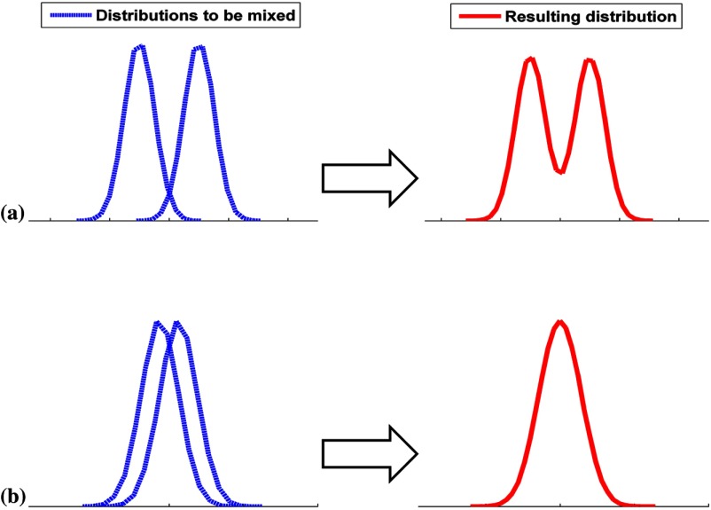
When all 54 phantoms were pooled, the distributions of the channel outputs were unimodal but they still deviate from a normal distribution, as shown in Figs. 6(c) and 8. One explanation for this is that the distribution of the channel outputs for each of the 54 phantoms was different, and the combined distribution thus was a continuous blending of a large number of the individual distributions with different centers and widths in contrast to the case of two phantoms. One way to think about this is as a Gaussian mixture model. The degree to which the resulting distribution is continuous depends on the width and distribution of centers of the individual Gaussians. For instance, consider the case of mixing two unimodal distributions. If the absolute value of the difference in their means (denoted by ) is much larger than the sum of their standard deviations (denoted by ), we expect the combined distribution to be bimodal.47 Figure 14 is a schematic showing the mixture of two Gaussians. When mixing more than two unimodal distributions, the number of modes in the resulting distribution depends on the extent to which the distributions overlap. This is based on the means and the standard deviations of the constituent distributions. It is not immediately evident how the number of phantoms affects the shape of the distribution for a particular channel outputs as this depends on the anatomical parameters of the phantoms as well as the channel used. It would thus appear prudent to check for normality and multimodality before applying model observers.
Fig. 14.
A schematic illustrating the mixture of two unimodal distributions. The rows are from the case of: (a) : the resulting distribution is thus bimodal and (b) : the resulting distribution is thus unimodal.
Furthermore, from the values of the correlation coefficient, skewness, and kurtosis reported in Tables 1–3, we observed that the degree of non-normality of the channel outputs changed from one channel to another. From Figs. 4–13, we observed that the shapes of the distributions from the two classes were different, indicating that the distribution for one class was not simply a shifted version of that for the other class. For example, variation in defect severity (see Fig. 10) produced a bimodal distribution for the defect-present class, while the defect-absent class had a unimodal distribution.
5.1. Central Limit Theorem
Since the channel outputs are the weighted sum of multiple random variables, it is often assumed that the channel outputs are MVN because of the CLT. However, the results presented above showed that this is not the case for the types of variations investigated. In this section, we provide more detailed discussions of reasons that the channel outputs had different degrees of departure from normality.
The simplest form of the CLT states that the arithmetic mean of a large number of independent and identically distributed random variables approaches a normal distribution under certain conditions.1,20,24 The basic assumptions of the CLT can be relaxed to various degrees resulting in different versions of the CLT with different degrees of generality.21–23 The degree of violation of the conditions of the CLT determines how well the mean of the random variables approximates a normal distribution.20,24–26 The details of these versions of the CLT are beyond the scope of this discussion. The key assumptions for the CLT that we will discuss are the (1) arithmetic mean of random variables, (2) large number of random variables, (3) identical distribution of random variables, and (4) independence of random variables. As discussed in the following, all the assumptions were violated simultaneously.
The first and second requirements are that a large number of pixels be summed with equal weights. The degree to which these requirements are satisfied depends on the details of the channel model. For the RSC used, the weights are very unequal and have different signs. The highest channel numbers tend to have very compact channels in the spatial domain, and approach delta functions, as shown in Fig. 3. Thus it is not surprising that the output of the sixth channel often deviated from normality. Furthermore, the different channels represent sets of weights with different degrees of nonuniformity, as shown in Fig. 3. It is clear from the results that the degree of non-normality of the channel outputs varies from one channel to another and sometimes produces bimodality, indicating that the CLT does not always hold (i.e., the channel outputs cannot always be approximated by a normal distribution).
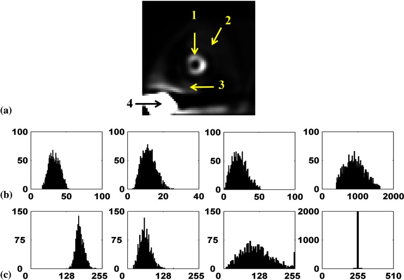
Regarding requirement (3), the random variables are not identically distributed (i.e., they have different means and variances) because they represent pixels with different activities from various organs. If a linear reconstruction method such as FBP is used, the reconstructed images will be MVN when neither background nor signal variability is present (i.e., MVN with different means and variances). When variability is present, the distribution of the pixels may no longer be MVN depending on the type of variability (i.e., possibly non-MVN with different means and variances). Due to their nonlinear nature, windowing and discretization will distort the distribution of the pixels (resulting in not only different means and variances but also different distribution shapes). To study requirement (3), we plotted the histograms of pixel values from four different positions in the image before and after windowing. The four positions were the anterolateral wall of the myocardium, the lung, the liver, and the gallbladder, respectively, with uptake variation without anatomical or signal variability (see Fig. 15). It is clear that the histograms are random variables with different means, standard deviations, and shapes. Before windowing, the shape of the distribution from different pixels was close to normal. After windowing and due to high activity in the gallbladder, its pixels are saturated to a gray level of 255 in the postprocessed MPS image; thus, the resulting histogram was a delta function as shown in Fig. 15(b).
Fig. 15.
(a) A noise-free short-axis image of a male phantom with small body, heart, and subcutaneous adipose thickness. The arrows indicate the four pixel locations used to compute the histograms. The four histograms from locations 1 to 4 are shown from left to right. Plots in (b) and (c) represent the histograms of the pixels (b) before windowing and (c) after windowing. The variations in pixel values are due to noise and uptake variations.
For many realistic medical images, requirement (4) is not satisfied because the pixels of the reconstructed images are correlated.48 Thus, the random variables that are combined are not independent. The postreconstruction low-pass filtering introduces additional correlations. Thus, the fourth requirement of the CLT was also violated. This does not necessarily mean that the channel outputs will be non-MVN. However, the various combinations of assumptions that are violated led, in many cases in this work, to deviation from normality. Figures 16 and 17 show the histograms and the Q–Q plots of the channel outputs with uptake variability for filter cutoffs 0.08 and . These figures show the combined effects of the violation of all the CLT requirements on the degree of deviation from normality.
Fig. 16.
Histogram plots of the channel outputs with uptake variability for different cutoffs. The axes are as described in Fig. 4. The columns represent the outputs from the six channels defined in Fig. 3. The rows are from cutoffs of (a) 0.08 and (b) . Sixty-four histogram bins were used.
Fig. 17.
Q–Q plots comparing the distributions of standardized channel outputs with the theoretical standard normal distribution for different cutoffs. The axes are as described in Fig. 5. The columns represent the outputs from the six channels defined in Fig. 3. The rows are for defect-present data with uptake variability having cutoffs of (a) 0.08 and (b) .
5.2. Rotationally Symmetric Frequency Channels Versus an Equally Weighted Channel
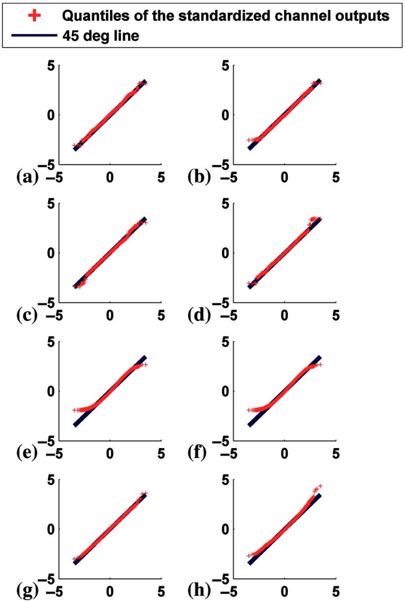
To illustrate the impact of using RSC, which had unequal weights, on the distribution of channel outputs, we considered the case of a uniform channel with equal weights in the spatial domain. The output from this channel represents the arithmetic mean of the images without and with uptake variability for a single phantom anatomy (male with the smallest value of all three anatomical parameters) as well as before and after the windowing step. Figure 18 shows the Q–Q plots for the output from this channel at cutoff frequencies of 0.08 and . This figure shows how the uptake variability and the filtering and windowing steps affected the distribution of the arithmetic mean. First, for the case of no uptake variability, the distribution of the mean was close to normal before and after windowing for both cutoffs (first and second rows of Fig. 18). Second, when uptake variability was present, the distribution of the mean deviates from normality, especially before windowing for both cutoffs (third row of Fig. 18). Finally, when uptake variability was present and the images were windowed, the distribution of the mean was closer to normal for the small cutoff (fourth row of Fig. 18). Thus, fulfilling requirements 1 and 2 of the CLT were not sufficient to ensure normality for some cases.
Fig. 18.
Q–Q plots comparing the distributions of standardized equally weighted channel outputs with the theoretical standard normal distribution for defect-absent class. The axes are as described in Fig. 5. The left and the right columns represent the cutoffs 0.08 and , respectively. The rows are from the cases of: (a) and (b) no uptake variability before windowing, (c) and (d) no uptake variability after windowing, (e) and (f) with uptake variability before windowing, and (g) and (h) with uptake variability after windowing.
5.3. Implications of Non-Normality of Channel Outputs on CHO Performance
Understanding the distribution of the channel outputs could help in the formulation of model observers and strategies for applying these observers in cases of background and signal variability. The principles of this study can also be applied to the case of efficient channels (i.e., channels used to approximate the IO) or the case of anthropomorphic channels (i.e., the CHO used to model human observer performance). The knowledge of the distribution of the channel outputs under various types of variability and processing could help in explaining the behavior of the CHO as compared to the IO and the human observer. For example, the CHO is the HO applied to the channel outputs. Thus, if channel outputs are not MVN, the performance of the HO will not be the same as the IO when these observers are applied to non-MVN channel outputs. In the following, we illustrate the use of the results of this work to develop strategies to apply CHOs to a population of realistic medical images.
For data such as the phantom population used here, the CHO template is estimated with ensemble methods. Since there are a finite number of images in the ensemble, the statistical precision of the CHO and resulting test statistics are limited. To address this, Wunderlich and Noo49–52 proposed an approach to estimate the CHO based on the incorporation of the knowledge of the channel outputs class means. The inclusion of this prior knowledge can help to reduce the statistical variability in the estimates of the CHO performance in case of a small number of images. This approach assumes that the channel outputs from both classes are MVN. However, as noted above, adding background or signal variability could result in violations of the MVN assumption.
The results of this work suggest that it may be desirable to use near continuous distributions of object parameters (e.g., the case of 54 phantoms) in order to avoid multimodal distributions of channel outputs. In case of signal and/or anatomical variability, the data indicate that the model observer study should be conducted in subsets with limited variability. For example, we can train and apply a set of observers to the channel outputs from groups of objects having signals or anatomies that obey or nearly obey the MVN assumption instead of training and applying a single observer to the channel outputs of all the objects.
6. Conclusions
The channel outputs used in CHOs are the weighted sums of many random variables; hence, the CLT is often assumed to imply that they will have MVN distribution. In this study, our goal was to investigate the validity of the MVN assumption of the channel outputs under both hypotheses for a binary classification task. This investigation was performed in the context of realistically simulated and postprocessed MPS images with different kinds of background and signal variations including noise level, anatomical, and signal variability.
The results showed that when neither signal nor anatomical variability was present, the distribution of individual channel outputs was close to normal, except for the highest frequency channel where the distribution was non-normal (negatively skewed). We observed that, for some combinations of variability, especially when the number of variations was small, the distribution of some of the channel outputs was sometimes multimodal. For example, in an image ensemble from two phantom anatomies or two signal locations, bimodal distributions were observed for both defect-absent and defect-present classes. When the variations were sampled from a more continuous distribution, such as a mixture of a large number of phantoms, the channel outputs were unimodal. However, even in these cases, the channel outputs were not always close to a normal distribution. One likely reason for this is that channel outputs computed using realistic medical images do not satisfy many of the requirements of the CLT.
The results reported in this paper showed that the channel outputs from both defect-absent and defect-present classes could deviate from normality and were sometimes multimodal depending on the type of variability. This suggests caution when applying the CHO to realistic medical images. In particular, the distribution of the channel outputs of both classes should be examined. Lastly, the results have implications in terms of strategies for applying the CHO to ensembles of images with background and signal variability.
Acknowledgments
This work was supported by the National Institutes of Health Grant Nos. R01 EB016231 and R01 EB013558. The content is solely the responsibility of the authors and does not necessarily represent the official views of the National Institutes of Health.
Biographies
Fatma E. A. Elshahaby holds BSc and MSc degrees in electronics and electrical communications engineering from Cairo University, Egypt. She also holds an MSc degree in electrical and computer engineering from Johns Hopkins University. Currently, she is pursuing her PhD in electrical and computer engineering at Johns Hopkins University. Her research interests include nuclear medicine imaging and task-based assessment of image quality.
Michael Ghaly is a postdoctoral fellow in the Division of Medical Imaging Physics of the Russell H. Morgan Department Radiology and Radiological Science at Johns Hopkins University. He received his PhD from the Department of Electrical and Computer Engineering at Johns Hopkins University. His research interests include myocardial perfusion SPECT imaging, task-based systems evaluation and optimization, tomographic reconstruction, and photon transport simulations.
Abhinav K. Jha is an instructor in the Division of Medical Imaging Physics of the Russell H. Morgan Department of Radiology and Radiological Sciences at Johns Hopkins University. He received his PhD from the College of Optical Sciences, University of Arizona. His research interests are in the design, optimization, and evaluation of medical imaging systems and algorithms using task-based quantitative image-science approaches.
Eric C. Frey is a professor in the Division of Medical Imaging Physics of the Russell H. Morgan Department Radiology and Radiological Science at Johns Hopkins University, with joint appointments in the Departments of Environmental Health Sciences and Electrical and Computer Engineering. His research is in the area of nuclear medicine, with applications to myocardial, neural and cancer imaging, targeted radiopharmaceutical therapy, and task-based assessment of image quality.
References
- 1.Barrett H. H., Myers K. J., Foundations of Image Science, Wiley, New York: (2004). [Google Scholar]
- 2.Barrett H. H., et al. , “Model observers for assessment of image quality,” Proc. Natl. Acad. Sci. U. S. A. 90(21), 9758–9765 (1993). 10.1073/pnas.90.21.9758 [DOI] [PMC free article] [PubMed] [Google Scholar]
- 3.Barrett H. H., et al. , “Linear discriminants and image quality,” Image Vision Comput. 10(6), 451–460 (1992). 10.1016/0262-8856(92)90030-7 [DOI] [Google Scholar]
- 4.He X., Park S., “Model observers in medical imaging research,” Theranostics 3(10), 774–786 (2013). 10.7150/thno.5138 [DOI] [PMC free article] [PubMed] [Google Scholar]
- 5.Hotelling H., “The generalization of student’s ratio,” Ann. Math. Stat. 2(3), 360–378 (1931). 10.1214/aoms/1177732979 [DOI] [Google Scholar]
- 6.Fisher R. A., “The use of multiple measurements in taxonomic problems,” Ann. Eugen. 7(2), 179–188 (1936). 10.1111/j.1469-1809.1936.tb02137.x [DOI] [Google Scholar]
- 7.Fukunaga K., Introduction to Statistical Pattern Recognition, 2nd ed., Academic Press, New York: (1990). [Google Scholar]
- 8.Barrett H. H., “Objective assessment of image quality: effects of quantum noise and object variability,” J. Opt. Soc. Am. A 7(7), 1266–1278 (1990). 10.1364/JOSAA.7.001266 [DOI] [PubMed] [Google Scholar]
- 9.Park S., et al. , “Channelized-ideal observer using Laguerre–Gauss channels in detection tasks involving non-Gaussian distributed lumpy backgrounds and a Gaussian signal,” J. Opt. Soc. Am. A 24(12), B136–B150 (2007). 10.1364/JOSAA.24.00B136 [DOI] [PMC free article] [PubMed] [Google Scholar]
- 10.Gallas B. D., Barrett H. H., “Validating the use of channels to estimate the ideal linear observer,” J. Opt. Soc. Am. A 20(9), 1725–1738 (2003). 10.1364/JOSAA.20.001725 [DOI] [PubMed] [Google Scholar]
- 11.Myers K. J., Barrett H. H., “Addition of a channel mechanism to the ideal-observer model,” J. Opt. Soc. Am. A 4(12), 2447–2457 (1987). 10.1364/JOSAA.4.002447 [DOI] [PubMed] [Google Scholar]
- 12.Wollenweber S. D., et al. , “Comparison of Hotelling observer models and human observers in defect detection from myocardial SPECT imaging,” IEEE Trans. Nucl. Sci. 46(6), 2098–2103 (1999). 10.1109/23.819288 [DOI] [Google Scholar]
- 13.Sankaran S., et al. , “Optimum compensation method and filter cutoff frequency in myocardial SPECT: a human observer study,” J. Nucl. Med. 43(3), 432–438 (2002). [PubMed] [Google Scholar]
- 14.Gifford H. C., et al. , “Channelized Hotelling and human observer correlation for lesion detection in hepatic SPECT imaging,” J. Nucl. Med. 41(3), 514–521 (2000). [PubMed] [Google Scholar]
- 15.Abbey C. K., Barrett H. H., “Human- and model-observer performance in ramp-spectrum noise: effects of regularization and object variability,” J. Opt. Soc. Am. A 18(3), 473–488 (2001). 10.1364/JOSAA.18.000473 [DOI] [PMC free article] [PubMed] [Google Scholar]
- 16.Park S., et al. , “Efficiency of human and model observers for signal-detection tasks in non-Gaussian distributed lumpy backgrounds,” Proc. SPIE 5749, 138 (2005). 10.1117/12.592238 [DOI] [Google Scholar]
- 17.Park S., et al. , “Efficiency of the human observer detecting random signals in random backgrounds,” J. Opt. Soc. Am. A 22(1), 3–16 (2005). 10.1364/JOSAA.22.000003 [DOI] [PMC free article] [PubMed] [Google Scholar]
- 18.Eckstein M. P., Abbey C. K., “Model observers for signal-known-statistically tasks (SKS),” Proc. SPIE 4324, 91 (2001). 10.1117/12.431177 [DOI] [Google Scholar]
- 19.Eckstein M. P., et al. , “Optimization of model observer performance for signal known exactly but variable tasks leads to optimized performance in signal known statistically tasks,” Proc. SPIE 5034, 123 (2003). 10.1117/12.480344 [DOI] [Google Scholar]
- 20.Rice J. A., Mathematical Statistics and Data Analysis, 3rd ed., Cengage Learning, Boston, MA: (2006). [Google Scholar]
- 21.Weber M., “A weighted central limit theorem,” Stat. Probab. Lett. 76(14), 1482–1487 (2006). 10.1016/j.spl.2006.03.007 [DOI] [Google Scholar]
- 22.Hilhorst H. J., “Central limit theorems for correlated variables: some critical remarks,” Braz. J. Phys. 39(2A), 371–379 (2009). 10.1590/S0103-97332009000400005 [DOI] [Google Scholar]
- 23.Rosén B., “On the central limit theorem for sums of dependent random variables,” Z. Wahrscheinlichkeitstheorie Verw. Geb. 7(1), 48–82 (1967). 10.1007/BF00532097 [DOI] [Google Scholar]
- 24.Wilcox R. R., Fundamentals of Modern Statistical Methods: Substantially Improving Power and Accuracy, 2nd ed., Springer, New York: (2010). [Google Scholar]
- 25.Bartoszyński R., Niewiadomska-Bugaj M., Probability and Statistical Inference, 2nd ed., Wiley, New Jersey: (2008). [Google Scholar]
- 26.Kevei P., “A note on asymptotics of linear combinations of iid random variables,” Period. Math. Hung. 60(1), 25–36 (2010). 10.1007/s10998-010-1025-7 [DOI] [Google Scholar]
- 27.Frey E. C., Gilland K. L., Tsui B. M., “Application of task-based measures of image quality to optimization and evaluation of three-dimensional reconstruction-based compensation methods in myocardial perfusion SPECT,” IEEE Trans. Med. Imaging 21(9), 1040–1050 (2002). 10.1109/TMI.2002.804437 [DOI] [PubMed] [Google Scholar]
- 28.Gilland K. L., et al. , “Comparison of channelized Hotelling and human observers in determining optimum OS-EM reconstruction parameters for myocardial SPECT,” IEEE Trans. Nucl. Sci. 53(3), 1200–1204 (2006). 10.1109/TNS.2006.870088 [DOI] [Google Scholar]
- 29.He X., et al. , “A mathematical observer study for the evaluation and optimization of compensation methods for myocardial SPECT using a phantom population that realistically models patient variability,” IEEE Trans. Nucl. Sci. 51(1), 218–224 (2004). 10.1109/TNS.2004.823331 [DOI] [Google Scholar]
- 30.He X., et al. , “Comparison of 180 degrees and 360 degrees acquisition for myocardial perfusion SPECT with compensation for attenuation, detector response, and scatter: Monte Carlo and mathematical observer results,” J. Nucl. Cardiol. 13(3), 345–353 (2006). 10.1016/j.nuclcard.2006.03.008 [DOI] [PubMed] [Google Scholar]
- 31.He X., Links J. M., Frey E. C., “An investigation of the trade-off between the count level and image quality in myocardial perfusion SPECT using simulated images: the effects of statistical noise and object variability on defect detectability,” Phys. Med. Biol. 55(17), 4949–4961 (2010). 10.1088/0031-9155/55/17/005 [DOI] [PMC free article] [PubMed] [Google Scholar]
- 32.Ghaly M., Links J. M., Frey E. C., “Optimization of energy window and evaluation of scatter compensation methods in myocardial perfusion SPECT using the ideal observer with and without model mismatch and an anthropomorphic model observer,” J. Med. Imaging 2(1), 1–14 (2015). 10.1117/1.JMI.2.1.015502 [DOI] [PMC free article] [PubMed] [Google Scholar]
- 33.Ghaly M., et al. , “Design of a digital phantom population for myocardial perfusion SPECT imaging research,” Phys. Med. Biol. 59(12), 2935–2953 (2014). 10.1088/0031-9155/59/12/2935 [DOI] [PMC free article] [PubMed] [Google Scholar]
- 34.Segars W. P., et al. , “4D XCAT phantom for multimodality imaging research,” Med. Phys. 37(9), 4902–4915 (2010). 10.1118/1.3480985 [DOI] [PMC free article] [PubMed] [Google Scholar]
- 35.Segars W. P., Tsui B. M. W., “MCAT to XCAT: the evolution of 4-D computerized phantoms for imaging research,” Proc. IEEE 97(12), 1954–1968 (2009). 10.1109/JPROC.2009.2022417 [DOI] [PMC free article] [PubMed] [Google Scholar]
- 36.Elshahaby F. E. A., et al. , “The effect of signal variability on the histograms of anthropomorphic channel outputs: factors resulting in non-normally distributed data,” Proc. SPIE 9416, 94160P (2015). 10.1117/12.2081629 [DOI] [Google Scholar]
- 37.Brankov J. G., “Evaluation of the channelized Hotelling observer with an internal-noise model in a train-test paradigm for cardiac SPECT defect detection,” Phys. Med. Biol. 58(20), 7159–7182 (2013). 10.1088/0031-9155/58/20/7159 [DOI] [PMC free article] [PubMed] [Google Scholar]
- 38.Henze N., Zirkler B., “A class of invariant consistent tests for multivariate normality,” Commun. Stat. Theory Methods 19(10), 3595–3617 (1990). 10.1080/03610929008830400 [DOI] [Google Scholar]
- 39.Henze N., Wagner T., “A new approach to the BHEP tests for multivariate normality,” J. Multivar. Anal. 62(1), 1–23 (1997). 10.1006/jmva.1997.1684 [DOI] [Google Scholar]
- 40.Looney S. W., “How to use tests for univariate normality to assess multivariate normality,” Am. Stat. 49(1), 64–70 (1995). 10.1080/00031305.1995.10476117 [DOI] [Google Scholar]
- 41.Dillon W. R., “The performance of the linear discriminant function in nonoptimal situations and the estimation of classification error rates: a review of recent findings,” J. Mark. Res. 16(3), 370–381 (1979). 10.2307/3150711 [DOI] [Google Scholar]
- 42.Rencher A. C., Methods of Multivariate Analysis, 2nd ed., Wiley, New York: (2003). [Google Scholar]
- 43.Kolmogorov A., “Sulla determinazione empirica di una legge di distribuzione,” Gior. Ist. Ital. Attuari 4, 83–91 (1933). [Google Scholar]
- 44.Frieden B. R., Probability, Statistical Optics and Data Testing: A Problem Solving Approach, 3rd ed., Springer Series in Information Sciences, Berlin: (2001). [Google Scholar]
- 45.Jha A. K., et al. , “Task-based evaluation of segmentation algorithms for diffusion-weighted MRI without using a gold standard,” Phys. Med. Biol. 57(13), 4425–4446 (2012). 10.1088/0031-9155/57/13/4425 [DOI] [PMC free article] [PubMed] [Google Scholar]
- 46.Thode H. C., Testing for Normality, 1st ed., CRC Press, New York: (2002). [Google Scholar]
- 47.Schilling M. F., Watkins A. E., Watkins W., “Is human height bimodal?” Am. Stat. 56(3), 223–229 (2002). 10.1198/00031300265 [DOI] [Google Scholar]
- 48.Wilson D. W., Tsui B. M. W., “Noise properties of filtered backprojection and ML-EM reconstructed emission tomographic images,” IEEE Trans. Nucl. Sci. 40(4), 1198–1203 (1993). 10.1109/23.256736 [DOI] [Google Scholar]
- 49.Wunderlich A., Noo F., “Estimation of channelized Hotelling observer performance with known class means or known difference of class means,” IEEE Trans. Med. Imaging 28(8), 1198–1207 (2009). 10.1109/TMI.2009.2012705 [DOI] [PMC free article] [PubMed] [Google Scholar]
- 50.Wunderlich A., Noo F., “New theoretical results on channelized Hotelling observer performance estimation with known difference of class means,” IEEE Trans. Nucl. Sci. 60(1), 182–193 (2013). 10.1109/TNS.2012.2227340 [DOI] [PMC free article] [PubMed] [Google Scholar]
- 51.Wunderlich A., et al. , “Exact confidence intervals for channelized Hotelling observer performance in image quality studies,” IEEE Trans. Med. Imaging 34(2), 453–464 (2015). 10.1109/TMI.2014.2360496 [DOI] [PMC free article] [PubMed] [Google Scholar]
- 52.Wunderlich A., Noo F., Heilbrun M., “New results for efficient estimation of CHO performance,” in Proc. 2nd Int. Conf. on Image Formation in X-ray CT, pp. 153–156 (2012). [Google Scholar]


