Integration of Administrative, Clinical, and Environmental Data to Support the Management of Type 2 Diabetes Mellitus

Abstract

A very interesting perspective of “big data” in diabetes management stands in the integration of environmental information with data gathered for clinical and administrative purposes, to increase the capability of understanding spatial and temporal patterns of diseases. Within the MOSAIC project, funded by the European Union with the goal to design new diabetes analytics, we have jointly analyzed a clinical-administrative dataset of nearly 1.000 type 2 diabetes patients with environmental information derived from air quality maps acquired from remote sensing (satellite) data. Within this context we have adopted a general analysis framework able to deal with a large variety of temporal, geo-localized data. Thanks to the exploitation of time series analysis and satellite images processing, we studied whether glycemic control showed seasonal variations and if they have a spatiotemporal correlation with air pollution maps. We observed a link between the seasonal trends of glycated hemoglobin and air pollution in some of the considered geographic areas. Such findings will need future investigations for further confirmation. This work shows that it is possible to successfully deal with big data by implementing new analytics and how their exploration may provide new scenarios to better understand clinical phenomena.

Big data are data “whose scale, diversity, and complexity require new architecture, techniques, algorithms, and analytics to manage it and extract value and hidden knowledge from it.”¹ As reported in our recent review, diabetes management may gain advantages from the big data revolution at least in 3 related research directions: clinical data mining on large data collections, home monitoring and distributed data management, and monitoring patients’ behavior and the impact of environmental factors.¹

In this article we show a case study aimed at jointly analyzing clinical, administrative, and environmental data of a cohort of around 1.000 patients, with the goal of unraveling potential spatiotemporal correlations between HbA1c and air pollution, as derived from satellites images.

The work has been carried on within the EU-funded MOSAIC project. Mosaic aims at providing new analytics to support the diagnosis and the follow-up of type 2 diabetes mellitus (DM) patients, so to improve their characterization and to help in evaluating the risk of developing complications related to type 2 DM (T2D). The project involves ten clinical and technical partners, from five European countries.

Within the EU funded MOSAIC project, we have created a data warehouse (DW) that integrates clinical information of 1.000 diabetic patients treated by the Fondazione Salvatore Maugeri (FSM) hospital in Pavia with the data gathered for administrative purposes (including visit prescriptions, drug purchases, hospital admission and discharge codes) by the local health care agency of Pavia. The DW provides a comprehensive time-oriented view of the individual patients’ histories.^1,2 One of the interesting features of the MOSAIC data sets is that, thanks to the information derived from secondary data, patients’ addresses are associated to precise municipality codes. Such geo-referencing features open the possibility to connecting environmental data to the clinical ones.

The join analysis of environmental and health-related information has been conceptualized as the Exposome.³ It has been recognized that, although expanding biomedical research capabilities, the combination of these wide-ranging data sources requires innovative approaches not only in data analysis but also in the visualization of their results.

Several epidemiological studies had investigated the association between air pollution and diabetes from different perspectives, and some of them have been recently reviewed.^4-6 Among these studies, some of them are focused on glucose control and on diabetes-related complications than in the onset or the mortality rate of the disease.^7,8 Another recent study⁹ shows a partly consistent link between long-term exposure to air pollution and the risk of T2D. The authors highlight that studies of air pollution exposure and T2D development have generated some significant association findings but also inconsistent results, maybe due to subpopulations and geographic heterogeneity. However, in evaluating the methods applied by previous studies, it become clear that possible enhancements to determine whether environmental factor are causally related to the onset of T2D or T2D metabolic control are related to the need of:

• Retrieving more evidence from longitudinal studies—take into account temporal aspects and fluctuations in chronic populations followed for several years/during the disease arise and progression

• Defining finer-scale models of air pollution

Our work, leveraging on the MOSAIC DW and on big-data enabled approaches to analyze satellites images, moves along the direction of improving the quality of clinical and environmental data analysis.

In our analysis we compute the mean HbA1c of each geographic area and evaluate its relation with air pollution. Since air pollution is a time-dependent variable, that is, it certainly depends on seasons and, in case of industrial pollution, on cycles of production, we performed a dynamic study of the correlation of glycemic control with air pollution. Hence we did not expressly focus on variability, but rather on the correlation between monthly behavior of glycemic control (measured as the HbA1c mean) and air pollution metric (estimated by remote sensing analysis). As also glycemic control may have a seasonal component, to verify if this correlation exists, we estimated and then removed the HbA1c seasonal components.

Data and Methods

Data and Population

The MOSAIC data set gathers two main data streams, previously collected for clinical and management purposes from 2009 to 2013. Clinical data from the FSM hospital consisted of demographic information (gender, birth date, time from diagnosis) physical examinations (BMI, blood pressure), and laboratory data, including HbA1c measurements and lipid profile. Administrative data include patients’ address, hospital admission and discharges, ambulatory encounters, and drug purchases.

We focused our analysis on the inhabitants of the Pavia Province, which is the area managed by the Local Health Care Agency.¹⁰ From the original MOSAIC cohort of 1020 T2D patients, we selected a subpopulation of 840 patients, for whom their addresses correspond to the considered geographic area. The Pavia Province is usually divided (for administrative and geographical reasons) into three main districts (Pavese, Lomellina, and Oltrepo), which in turn are divided into nine counties. Figures 1a and 1b show Pavia Province and its partition into counties.

Figure 1.

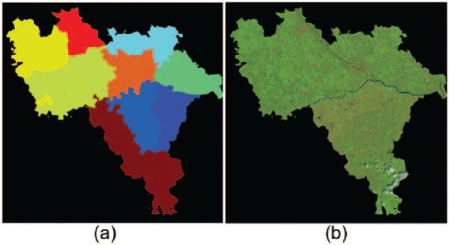
Pavia Province: satellite map (a) and counties (b).

Within this context, we examined whether HbA1c levels of the studied population showed seasonal fluctuations and, in the case these variations were significant, if they are correlated to air pollution measurements as derived from satellites data.

Spatiotemporal Scales

The first step in the analysis was to tackle heterogeneous and diverse dimensionalities of the data streams, to use them in a common analysis framework. Compared to traditional cross-sectional studies, this phase was particularly challenging as we studied the relationship between variables evolving during time. Both HbA1c and air pollution are strongly time-dependent. On one hand, chronic patients are likely to evolve through several disease complexity levels, on the other hand, pollution levels may change due to land transformation, like building new residential areas or changes in industrial strategies.

Therefore, one of the main efforts was to define the level of detail through which derive meaningful patterns and observe events of interest. We considered temporal and spatial aspect of clinical and satellite data. Table 1 shows the dimensionalities of the two data streams, from fine scale to coarse scale.

Table 1.

Spatiotemporal Granularities Schema.

		Finer granularity	→		Coarser granularity
Spatial	Clinical data	Municipality	Districts	County	Pavia Province
	Satellite data	Pixel	Districts	County	Whole world
Temporal	Clinical data	Months (visit frequency)	Seasons		10 years
	Satellite data	Weeks (satellite cycles)	Seasons		5 years

In this context, we selected an approach able to balance aggregated data (over the whole geographic area; for the entire observation period) and punctual data (a pixel value; a single HbA1c measure taken in a certain day). This approach is based on the detection of seasonal variations within counties.

HbAc Longitudinal Analysis

Once geographic boundaries and temporal scales were defined, we calculated average HbA1c values in each county for each year, to assess glycemic control seasonal variations. Differently from other studies^11-14 aimed at providing evidence of cyclic variations in glycemic control in the whole population, the main focus of our approach was to assess seasonal Hab1c variability within each county. We therefore calculated mean HbA1c values grouped by seasons in each county population. As results, seasonal Hab1c levels of the nine geographic areas were defined for each year from 2009 to 2014.

To retrieve significant fluctuations of HbA1c and select the patterns to further investigate, we performed a mixed effect analysis (implemented in the R package; http://cran.r-project.org/web/packages/lme4/index.html).¹⁵ The applied methods allowed selecting significant (P value < .05) HbA1c seasonal geo-localized variations during the observation period.

HbA1c Time-Series Analysis

As already stated, the main aim of this work is to select the counties showing higher HbA1c variations in specific years. To separate the time series of the counties from the HbA1c seasonal component that is present in the entire province, we applied the additive model of seasonal decomposition procedure.^16,17 From un-aggregated time series we extracted monthly variations of HbA1c profiles (Figure 2). The extraction of seasonal adjustment factors allowed identifying months with peaks. Consequently, original time series of each county were adjusted and smoothed by removing this factor.

Figure 2.

Time series decomposition and monthly factor for the whole data set (Pavia Province, 2009-2014). X-axis indicates years, y-axis the monthly mean value of HbA1c.

This procedure was meant to reduce the effects that are present every year and independently from the specific county; for example, the December month has an additive seasonal component of nearly 8 mmol/mol, showing the possible effect of lack of exercise maybe due to the autumn season and worsening of diet due to the winter period in the whole population.

Air Pollution Satellites Maps

The correlation between the presence of black particulate and the recorded temperature can be thoroughly characterized by radiance processes that affect the energy transmission throughout the atmosphere. Specifically, a pollution layer delivers a decrease in the atmospheric transmission factor. This effect impacts the thermal infrared acquisition, since the solar heating is decreased as well. Consequently, the emitted radiance is lower, that is, the signal recorded by the sensor is lower. Simultaneously, the pollution layer absorbs the emitted radiance, that is, causes a strong impoverishment of the energy that is radiated upward. Hence, the aforementioned physical processes contribute to outline the correlation between the increase of pollution and the decrease of apparent temperature. Then, we assume that pollution plays a key role in the thermal pattern of a remotely sensed scene, that is, exploit the air quality maps from the aforementioned images.¹⁸

Several models have assessed the magnitude of these processes and their effects.¹⁹ Collecting the data over the thermal infrared band and plotting them with reference to the black particulate concentration as reported by ground stations, it is apparent as the physical processes that affect the radiance transmission and absorption drive the correlation between air pollution and temperature records. Specifically, the energy that is scattered by the instantaneous field of view is used before any image preprocessing is employed, that is, the contribution provided by the environment is fully considered. The aforesaid reflectance records are called raw counts. Moreover, to provide a thorough and reliable characterization of the aforementioned interplay, while avoiding the contribution delivered by other environmental pollutants, the concentration of particulate matter with aerodynamic diameter smaller than 10 μm (ie, PM10) is considered. Hence, taking into account the overall pattern of the raw counts thermal signal as a function of black particulate concentration, a polynomial fitting model has been implemented to estimate the air quality of the scene.¹⁸

On the other hand, to match the region of the remotely sensed data with the Pavia second order administrative area, we implemented spectral analysis throughout the years 2009-2014. Specifically, to achieve the air quality maps, the data acquired by LandSat L8 mission by means of operational land imager (OLI) and thermal infrared sensor (TIRS) have been considered. Furthermore, the Pavia second order administrative area is spread over a region of 2968.64 km² in northwestern Italy; it counts 189 municipalities.

We collected 35 LandSat images in the above-mentioned temporal interval over this test location, where each LandSat image consists of 2800 × 2800 pixels and has a 30 m spatial resolution. Then, for each temporal series we considered the thermal infrared signals acquired by LandSat 8 over the areas covered by the ground probes that have been taken into account. Then, we have been able to draw a polynomial relationship between black particulate concentrations and sensed reflections. Hence, for each pixel in every temporal series, we apply the polynomial function resulting from the aforementioned fitting process to estimate the air quality, which has been quantized on 50 levels over the black particulate concentration estimate.^18-20

Figure 3 reports the thermal infrared raw counts of the images collected on the four seasons in the 2009-2014 interval as a function of the black particulate PM10 concentration as recorded by the aforementioned ground stations that are located in Pavia and 4 towns within its second order administrative area (ie, Voghera, Vigevano, Parona, Sannazzaro de’ B.). Such area is grouped for health care purposes into three districts, Pavese (including Pavia), Lomellina (comprising Vigevano, Parona and Sannazzaro de’ B.), and Oltrepo’ (including Voghera). Apparently, Figure 3 shows how the black particulate concentration impacts on the recorded reflectance signals according to the aforementioned thermal infrared effects provided by air pollution. Thus, it is possible to infer air quality maps by properly processing the remotely sensed images according to the scheme that has been previously introduced. Specifically, we aim at characterizing the air quality of the given scene according to the quantization that is proposed at the bottom of Figure 3. Finally, Figure 3 displays also the polynomial fitting between black particulate concentration and raw counts provided by remotely sensed thermal infrared imagery as a solid black line. It is worth to note that the aforementioned fitting can be considered as very accurate and reliable, as its confidence coefficient R² reached the value of .9.

Figure 3.

Raw counts of the thermal infrared data of LandSat L8 images acquired over path 194 row 29 orbit on the 4 seasons in the 2009-2014 interval as a function of the black particulate PM10 concentration as recorded by the Pavia second order administrative area ground stations (located in Pavia, Voghera, Vigevano, Parona, and Sannazzaro de’ B.). Polynomial fitting between black particulate concentration and raw counts of the thermal infrared imagery is also reported: its confidence coefficient R² reached the value of .9.

Results

Characteristics of Studied Population and Counties

Tables 2 to 4 report the basic characteristics of the patients taken into consideration in the 5 years period, including sex, age, time from diagnosis, BMI, HbA1c, distribution per residence address, and values of HbA1c and PM10 per county. It is possible to notice an uneven distribution of sex and patient distribution in the districts and a very slight worsening of the clinical conditions. Mean HbA1c and Air pollution values vary within the counties, while there is no apparent correlation between the two.

Table 2.

Population Characteristics at Baseline and Follow-Ups.

	Baseline (2009)		Follow-up (2009-2014)
	Mean	SD	Mean	SD
BMI	29.31	4.84	29.68	5.25
HbA1c (mmol/mol)	52.44	12.10	54.47	12.15
Age, years	63.86	9.94	65.32	9.92
Time from diagnosis, years	8.92	8.80	9.66	8.61

Table 4.

Air Pollution Values in the Counties.

District	County	Mean HbA1c values (mmol/mol)	Mean air pollution values (PM10 µg/m3)
Pavese	Certosa	53.26	25.17
Pavese	Corteolona	55.11	24.83
Pavese	Pavia	53.75	25.13
Lomellina	Garlasco	56.70	27.25
Lomellina	Mortara	50.93	23.78
Lomellina	Vigevano	62.66	20.77
Oltrepo	Broni	60.30	25.43
Oltrepo	Casteggio	54.56	25.71
Oltrepo	Voghera	57.70	20.91

Table 3.

Population Characteristics at Baseline.

	Follow-up (2009-2014), 840 pts
Gender (%)
Female	40.96
Male	59.04
Smoking habit (%)
Yes (current and former)	51.08
No	48.92
Residence address (%)
Pavese	69.05
Lomellina	13.33
Oltrepo	17.62

Significant HbA1c Variations and Correlation With Air Pollution

After having applied time series decomposition methods to the data of the whole area, and having removed the shared seasonality factors, we ran the mixed effect model to select those counties and years showing significant HbA1c fluctuations among seasons. The selected counties and years are shown in Table 5. Subsequently, we obtained air quality values and maps from the LandSat images using the same spatiotemporal scale. Figure 4 shows the results for years 2011 and 2012.

Table 5.

Counties and Years for Which Mean HbA1c Seasonal Values Were Significantly Different From the Mean.

District	County	Year	P value
Pavese	Certosa	2011	.00088
Pavese	Certosa	2012	.00034
Pavese	Pavia	2011	.00005
Pavese	Pavia	2012	.00009
Lomellina	Garlasco	2011	.00046
Oltrepo	Casteggio	2012	.00921

Figure 4.

Air quality maps for 2011 and 2012. The same air quality color map in Figure 3 applies here.

The next steps of the analysis were devoted to compare these finding in each area and period of interest to detect possible correlations between Hb1c variations and changes in air pollution. In particular, we wanted to evaluate if, in certain counties, notable seasonal fluctuations of HbA1c can be correlated with the air pollution pattern in a certain year.

We found correlations in all counties reported in Table 4 (Certosa, Pavia, Garlasco, and Casteggio). In the following we will detail the results obtained in Pavia County, which is the one with the largest number of patients, since it is where the FSM hospital is located. Furthermore, Pavia County has the most homogenous geography.

Table 6 shows the P values of the HbA1c patterns calculated through the mixed effect model test for each year as well as the correlation between the HbA1c mean seasonal values and seasonal air pollution.

Table 6.

Results of Mixed Effect Model Analysis for Each Year in Pavia County and Correlation of HbA1c and Air Quality Values.

	Year	HbA1c patterns	HbA1c air quality correlation
Pavia	2009	n.s.	−.029
Pavia	2010	<.05	.66
Pavia	2011	<<.01	.94
Pavia	2012	<<.01	.81
Pavia	2013	<.01	.83
Pavia	2014	ns	.37

Once the seasonal component has been removed, it is necessary to understand if there are temporal patterns in both HbA1c and air pollution, and if these temporal pattern are still correlated.

Figure 5 shows that when there are significant temporal patterns in the residual HbA1c, such patterns are correlated to air pollution, and that the more this temporal pattern are significant the higher is the correlation.

Figure 5.

HbA1c pattern P values (in log scale) and their correlations with seasonal air pollution patterns.

As an example, we can see (Figure 6) that in Pavia County during 2011 HbA1c and air pollution values followed the same trend:

Figure 6.

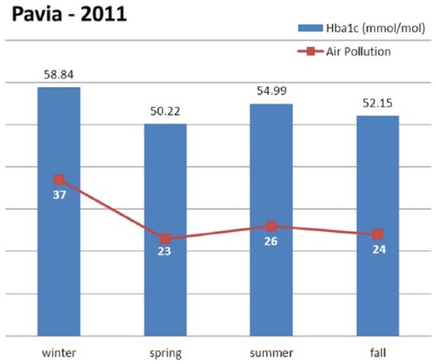
HbA1c and air pollution trends in Pavia County during 2011. The air pollution estimates are delivered in terms of a digitalized scale retrieved from the air quality class metric in Figure 3 as quantized in 50 intervals.

• HbA1c, compared with the year mean value (54.05 mmol/mol), shows higher values during winter, lower values in spring and fall, and slightly higher values in summer.

• Air pollution (on a 0-50 scale), compared with the year mean value (27.5 mmol/mol), shows the same trend.

Discussion

It is of course important to highlight that the analysis shown in this article is a proof of concept. In particular, we have clearly shown that, thanks to data availability and big data technologies, it is now possible to jointly study heterogeneous data, such as health care and air pollution information extracted from satellites. This provides an unprecedented opportunity to improve our understanding of phenomena by extracting unseen temporal and spatial correlations.

In the case study taken into consideration, we hypothesize the presence of a relationship between the HbA1c seasonal patterns and air pollution patterns in some areas of the Pavia Province. Such hypothesis has some clinical justifications,⁸ although the evidence supporting it needs further confirmation. The analysis of the data carried on in the Pavia Province certainly supports the presence of spatiotemporal correlation patterns.

We are of course aware of the possible biases that this approach may entail:

1. As we based our analysis on retrospective data derived from periodic visit patients underwent, we don’t have repeated measures for each subject for each season (1 single measure of each patient in each season) and there are possible confounding effects due to scheduled visits for more complicated patients; moreover, the areas under consideration have different population densities. Other confounding effects may derive from the treatments to which the chronic population is exposed and from patients’ compliance to therapies.

2. HbA1c values represent the summary of the patients’ glucose metabolism in the previous months. Therefore, the average seasonal values include a delayed clinical effect that causes an overlap between seasons. As such, the correlations would need to be verified with a larger population and testing also cross-correlation indexes on a time continuous scale.

Conclusions

The availability of large data collections concerning long-term monitoring of diabetes patients is a strong push toward the definition of “diabetes analytics” platforms. While several solutions are now available to interpret home-monitoring data, in particular in type 1 diabetes, there is need of defining new methods and tools able to extract useful information from large sets of heterogeneous information, such as clinical, administrative and environmental data. Rather interestingly, such information may be readily available by combining the content of electronic medical records with open data, such as satellites images. In this article we have shown an example of large-scale diabetes analytics, which can be exploited to generate interesting hypotheses as well as to highlight temporal and spatial patterns in diabetes control. Future steps will involve the definition of software tools and control dashboard that will include in the analytic platforms advanced visualization solutions for the benefit of health care providers and decision makers.

References

- 1. Bellazzi R, Dagliati A, Sacchi L, Segagni D. Big data technologies: new opportunities for diabetes management. J Diabetes Sci Technol. 2015;9(5):1119-1125. [DOI] [PMC free article] [PubMed] [Google Scholar]
- 2. Dagliati A, Sacchi L, Bucalo M, Segagni D, Zarkogianni K, Martinez-Millana A. A data gathering framework to collect type 2 diabetes patients data. In: IEEE-EMBS international conference on Biomedical and Health Informatics (BHI), Valencia, 1-4 June 2014, pp.244-247. [Google Scholar]
- 3. Martin Sanchez F, Gray K, Bellazzi R, Lopez-Campos G. Exposome informatics: considerations for the design of future biomedical research information systems. J Am Med Inform Assoc. 2014;21(3):386-390. [DOI] [PMC free article] [PubMed] [Google Scholar]
- 4. Rajagopalan S, Brook RD. Air pollution and type 2 diabetes mechanistic insights. Diabetes. 2012;61:3037-3045. [DOI] [PMC free article] [PubMed] [Google Scholar]
- 5. Thiering E, Heinrich J. Epidemiology of air pollution and diabetes. Trends Endocrinol Metab. 2015;26(7):384-394. [DOI] [PubMed] [Google Scholar]
- 6. Janghorbani M, Momeni F. Systematic review and metaanalysis of air pollution exposure and risk of diabetes. Eur J Epidemiol. 2014;29(4):231-242. [DOI] [PubMed] [Google Scholar]
- 7. Chuang K, Yan Y, Chiu S, Cheng T. Long-term air pollution exposure and risk factors for cardiovascular diseases among the elderly in Taiwan. Occup Env Med. 2011;68(2):64-68. [DOI] [PubMed] [Google Scholar]
- 8. Tamayo T, Rathmann W, Krämer U, Sugiri D, Grabert M, Holl RW. Is particle pollution in outdoor air associated with metabolic control in type 2 diabetes? PLOS ONE 2014;9(3):e91639. [DOI] [PMC free article] [PubMed] [Google Scholar]
- 9. Park SK, Adar SD, O’Neill MS, et al. Long-term exposure to air pollution and type 2 diabetes mellitus in a multiethnic cohort. Am J Epidemiol. 2015;181(5):327-336. [DOI] [PMC free article] [PubMed] [Google Scholar]
- 10. Dalle Carbonare S, Cerra C, Bellazzi R. Development and representation of health indicators with thematic maps. Stud Health Technol Inform. 2012;180:220-224. [PubMed] [Google Scholar]
- 11. Gikas A, Sotiropoulos A, Pastromas V, Papazafiropoulou A, Apostolou O, Pappas S. Seasonal variation in fasting glucose and HbA1c in patients with type 2 diabetes. Prim Care Diabetes. 2009;3(2):111-114. [DOI] [PubMed] [Google Scholar]
- 12. Hill NR, Peters CJ, Thompson RJ, Matthews DR, Hindmarsh PC. Cyclical variation in HbA1c values during the year: clinical and research implications. Diabetes Care. 2013;36(10):175-176. [DOI] [PMC free article] [PubMed] [Google Scholar]
- 13. Sakura H, Tanaka Y, Iwamoto Y. Seasonal fluctuations of glycated hemoglobin levels in Japanese diabetic patients. Diabetes Res Clin Pract. 2010;88(1):65-70. [DOI] [PubMed] [Google Scholar]
- 14. Tseng CL, Brimacombe M, Xie M, et al. Seasonal patterns in monthly hemoglobin A1c values. Am J Epidemiol. 2005;161(6):565-574. [DOI] [PubMed] [Google Scholar]
- 15. Baayen RH, Davidson DJ, Bates DM. Mixed-effects modeling with crossed random effects for subjects and items. J Mem Lang. 2008;59(4):390-412. [Google Scholar]
- 16. Cleveland RB, Cleveland WS, McRae JE, Terpenning I. STL: a seasonal-trend decomposition procedure based on loess. J Off Stat. 1990;6(1):3-73. [Google Scholar]
- 17. Keeling CD, Bacastow RB, Bainbridge AE, et al. Atmospheric carbon dioxide variations at Mauna Loa Observatory, Hawaii. Tellus. 1976;28(6):538-551. [Google Scholar]
- 18. Wald LB. Observing air quality over the city of Nantes by means of LandSat thermal infrared data. Int J Remote Sens. 1999;20(5):947-959. [Google Scholar]
- 19. Wald L, Basly L, Baleynaud J. Satellite data for the air pollution mapping. In: Proceedings of the 18th EARSeL symposium on operational remote sensing for sustainable development, Enschede, The Netherlands, 11-14 May 1998, pp.133-139. [Google Scholar]
- 20. Marinoni A, Gamba P. Big data for human-environment interaction assessment: challenges and opportunities. In: Proceedings of the ESA Big Data Space conference (BiDS), Frascati, Italy, November 2014, pp.1-4. [Google Scholar]