Attracting cavities for docking. Replacing the rough energy landscape of the protein by a smooth attracting landscape

Abstract

Molecular docking is a computational approach for predicting the most probable position of ligands in the binding sites of macromolecules and constitutes the cornerstone of structure‐based computer‐aided drug design. Here, we present a new algorithm called Attracting Cavities that allows molecular docking to be performed by simple energy minimizations only. The approach consists in transiently replacing the rough potential energy hypersurface of the protein by a smooth attracting potential driving the ligands into protein cavities. The actual protein energy landscape is reintroduced in a second step to refine the ligand position. The scoring function of Attracting Cavities is based on the CHARMM force field and the FACTS solvation model. The approach was tested on the 85 experimental ligand–protein structures included in the Astex diverse set and achieved a success rate of 80% in reproducing the experimental binding mode starting from a completely randomized ligand conformer. The algorithm thus compares favorably with current state‐of‐the‐art docking programs. © 2015 The Authors. Journal of Computational Chemistry Published by Wiley Periodicals, Inc.

Introduction

Molecular docking is a computational approach for predicting the most probable binding geometries of small molecules on macromolecular targets. Docking programs, which predict possible structures for ligand–target complexes and sometimes estimate the corresponding binding affinities, constitute the cornerstone of structure‐based computer‐aided drug design (SB‐CADD). A docking program generally consists of a sampling algorithm and a scoring function.1, 2, 3 The sampling algorithm generates possible positions for the ligand on the protein surface, while the scoring function evaluates the goodness‐of‐fit to rank these putative binding modes and finally identifies the one most likely to correspond to the native, experimental, binding mode.

A large number of sampling algorithms have been developed over the last decades. They can roughly be divided into three major categories: incremental reconstruction, stochastic search, and simulation approaches.2

In incremental reconstruction, the molecule is divided into a single rigid fragment and several shells of flexible extensions. The rigid fragment, selected for its ability to make the highest number of interactions with the receptor or for its central position in the ligand, is docked first. The flexible moieties are then reconnected incrementally.4, 5, 6 A variant consists in decomposing the molecule into several fragments that are docked independently and later fused into the active site.7, 8, 9, 10, 11, 12

Stochastic methods consider the ligand as a whole. Here, the degrees of freedom for the ligand docking, e.g., the global translation and rotation of the ligand in Cartesian space and the values of the bond lengths, bond angles, and dihedral angles are energy optimized using different approaches such as evolutionary algorithms (EA),13, 14, 15, 16, 17 Monte Carlo (MC) algorithms,18, 19, 20, 21 or swarm intelligence (SI) approaches.22, 23, 24, 25

Simulation approaches consist in molecular dynamics simulations and geometry optimization methods to minimize the energy of the ligand–target complex. These approaches are generally unable to cross high‐energy barriers of ligand–protein interaction. Therefore, the ligand–target complex geometry is often trapped in local energy minima corresponding to nonnative binding geometries,26 although it was shown recently that the global minimum can be determined using replica exchange simulations in some cases.27 As a consequence, simulation approaches are seldom used as stand‐alone sampling algorithms. However, they can efficiently improve other search methods by locally refining poses suggested by MC‐, EA‐, or SI‐based algorithms, for instance. This approach is used, for example, in AutoDock,15 AutoDock Vina,19 ICM,28 DOCK,10 or EADock.6, 13, 14

Energy minimization algorithms yield an inefficient sampling procedure as the energy landscape is dominated by the 1/r ⁻¹² repulsive component of the Lennard–Jones potential, with no driving force toward the protein surface. To circumvent this problem, we tuned the energy landscape by replacing the rough repulsive protein landscape by a smooth attractive landscape generated by virtual attracting points placed on a cloud surrounding the protein. In this so‐called attracting cavity landscape, the energy minimizations not only drive the system very efficiently toward binding cavities but are also much faster since the atoms of the protein are no longer present. Once the algorithm has found a favorable conformation in the attracting cavity landscape, the ligand conformation can be optimized in the actual protein landscape to provide the final adjustments and to obtain a reliable energy value. Here, we describe a simple ligand–protein docking algorithm, called “Attracting Cavities” (AC). The sampling procedure of AC is constituted only of ligand energy minimizations in the attracting cavity landscape, and its scoring function is based on the CHARMM29 force field and the FACTS solvation model.30 Although AC has been tested for rigid‐protein docking, it can be modified to account for the flexibility of the protein.

After describing the method, we test AC on the 85 experimental ligand–protein structures of the Astex diverse set31 and compare to state‐of‐the art docking programs.

Methods

Docking algorithm of the attracting cavities approach

In the AC approach, the direct docking of a small molecule in the “actual” energy landscape of the protein (blue arrow in Fig. 1) is replaced by the following procedure (red arrows in Fig. 1):

Figure 1.

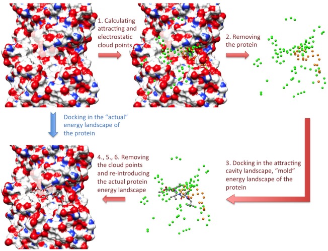
AC algorithm. The attracting and electrostatic cloud points are shown as green and orange spheres, respectively. The numbering of the arrows corresponds to the description of the algorithm given in the text.

1. First, two sets of points situated in the cavities and at the surface of the protein are calculated. The points of the first set, called the attracting cloud, are fitted with the attractive part of a Lennard–Jones potential. The points of the second set, called the electrostatic cloud, are fitted not only with the same attractive part of a Lennard‐Jones potential but also with a charge mimicking the electrostatic potential created by the protein charges on that point.

2. The protein is then removed, while the cloud points are kept, creating a “mold” potential of the protein.

3. The ligand conformation is stretched by applying 500 steps of the adopted‐basis Newton Raphson (ABNR) energy minimization algorithm after imposing a +0.2e charge on all atoms. The ligand native partial charges are reintroduced after this minimization, before performing the sampling. The ligand principal axes are aligned with the x, y, and z axes, and the ligand is subsequently centered on each point of the attracting cloud, in all the orientations obtained by systematic and combinatorial rotations along the x, y, and z directions. The rotation step can be 45°, 60°, or 90°, defining the sampling thoroughness. Starting from each position and orientation, the ligand is minimized by 1500 steps of ABNR algorithm, in the energy landscape created by the two clouds. The simple potential energies created by the points of the attracting and electrostatic clouds create a smooth and mainly attractive potential. This allows the ligand to easily reach positions corresponding to local energy minima (e.g., fitting inside protein cavities with complementary shape and charges) by energy minimization. A soft‐core correction is applied to the electrostatic and van der Waals potentials of the cloud points to prevent energetic divergence when ligand atoms are superimposed to them.

4. Then, the cloud points are removed, and the protein force field is reintroduced in two steps. First, the ligand, starting from each position determined in step 3, is energy‐minimized by 1000 steps of ABNR while the protein is described by a soft‐core potential. This procedure intends to correct steric clashes caused by reintroduction of the protein.

5. Subsequently, the ligand, starting from each position determined in step 4, is energy‐minimized using 200 steps of ABNR in the protein energy landscape, as established by the CHARMM22 or CHARMM27 force field without any correction. The ligand is flexible during the minimization procedures of steps 4 and 5.

6. Finally, the ligand positions generated in step 5 are ranked according to the EADock13 scoring function32, 33 that accounts implicitly for solvation energy. Binding modes are clustered based on their Cartesian coordinates, with a 2 Å cluster radius. For this, the top‐ranked binding mode is chosen as center for the first cluster. Binding modes closer than 2 Å from it are assigned to this first cluster. The next most favorably ranked binding mode is chosen as the center for the second cluster, and its neighbors are assigned to this second cluster. This procedure continues until all binding modes have been assigned to a cluster. Lastly, a maximum of eight members are kept in each cluster. The remaining members, corresponding to the less favorably scored binding mode in each cluster, are discarded to limit the size of the output. The score of a cluster corresponds to the average energy of its three top‐scored members, to limit the risk that a few complexes penalize the whole cluster. This clustering and scoring procedure was taken from that of EADock,13 which shares the same scoring function. EADock was developed and benchmarked using the Ligand Protein Databank (LPDB)34 and not the Astex dataset. Therefore, this procedure was not optimized to increase the success rate of AC on the Astex dataset, limiting the risk of overfitting.

Determination of attracting cloud points

A simple geometric algorithm is used to define the points of the attracting cloud. First, the search space, which is defined as an orthorhombic box whose center and size are chosen by the user, is filled with a 1 Å cubic lattice. Each lattice point is surrounded by two spheres of radius R _in and R _out, with R _out > R _in. A grid point is chosen to be an attracting point if the number of protein heavy atoms in the inner sphere (N _in) is null, if the number of protein heavy atoms in the outer sphere (N _out) is larger than a chosen threshold value (N _Thr), and if it is not closer than 1.5 Å from another attracting point (Fig. 2). R _in, R _out, and N _Thr are parameters of the method, while N _in and N _out are calculated values for a given position in space.

Figure 2.

Algorithm to determine the attracting cloud points. Brown crosses represent example grid points surrounded by their inner (brown) and outer (green) spheres of radius R _in (3.2 Å) and R _out, (8.0 Å) respectively. Protein atoms are shown as van der Waals spheres. A grid point is elected attracting point if the number of protein heavy atoms in the inner sphere (N _in) is null, if the number of protein heavy atoms in the outer sphere is larger than N _Thr, and if it is not closer than 1.5 Å from another attracting point. Large values of N _Thr (70 and above) strictly concentrate attracting points in protein cavities, while smaller values (50 to 60) extend the distribution to less concave regions of the protein surface. Even smaller N _Thr values allow covering the entire surface of the protein, including convex regions. [Color figure can be viewed in the online issue, which is available at wileyonlinelibrary.com.]

The N _in = 0 condition excludes points within the volume occupied by the protein. A value of 3.2 Å was determined for R _in. This is 0.2 Å smaller than the smallest sum of van der Waals radii for two protein heavy atoms in the CHARMM force field, i.e., 2 × 1.7 Å for two backbone oxygen atoms. This value was used to fill even small yet relevant cavities with attracting points. The second condition, N _out ≥ N _Thr, concentrates the attracting points close to the protein and provides a simple mean to fine‐tune the sampling procedure so that docking focuses more on deep protein cavities or, on the contrary, also includes less concave regions, such as shallow grooves on the protein surface (Figs. 2 and 3). Large values of N _Thr concentrate attracting points in protein cavities, while smaller values extend the distribution to less concave portions of the protein surface. Very small N _Thr values allow covering the entire surface of the protein, including convex regions. Focusing the sampling algorithm on protein cavities increases the docking speed but might lead to sampling failures in case the experimental binding mode is not inside a well‐defined and buried binding pocket. A value of 8 Å was arbitrarily chosen for R _out. This value of R _out was found to be large enough to locate a significant number of protein atoms (N _out) in the corresponding sphere and small enough to consider only the topology of the protein around the lattice point. Since the effect of the R _out and N _Thr values are linked, we only tested the influence of N _Thr. Values of 50, 60 and 70 for N _Thr were found to provide the best compromise between speed and sampling thoroughness given this R _out value.

Figure 3.

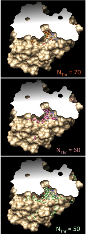
Distribution of attracting points on the surface of HSP90 (2BSM in the PDB), as a function of N _Thr. Attracting points calculated using N _Thr = 70, 60, and 50 are shown as orange, pink, and green spheres, respectively. The experimental position of the HSP90 ligand is shown in thick line to locate the binding pocket. N _Thr = 70 concentrates the attracting points in the binding pocket, while N _Thr = 50 extends the distribution to all protein invaginations. The distributions were calculated with R _in = 3.2 Å and R _out = 8.0 Å. [Color figure can be viewed in the online issue, which is available at wileyonlinelibrary.com.]

Determination of electrostatic cloud points

The points of the electrostatic cloud are chosen in the close vicinity of the protein surface. First, the orthorhombic search space is filled with a 1.5 Å cubic lattice. To be further considered, a lattice point must be situated at a distance larger than R_p + 0.3 Å from any protein atom (where R_p is the van der Waals radius of the protein atom) and smaller than R_p + 0.6 Å from at least one protein atom. The pseudo‐charge of each retained lattice point, C _lp, is calculated as C _lp = ζ × E_p, where E_p is the electrostatic potential created by the protein on the point, and ζ = 0.01e kcal⁻¹ mol. Finally, the lattice point is selected as part of the electrostatic cloud if the absolute value of its charge, C _lp, is larger than 1.2e. This limits the number of points in the electrostatic cloud so as to create a smooth energy landscape.

Energy calculation and scoring

All energy calculations were performed with the CHARMM29 Molecular Mechanics package versions 34a1 and 36b1. The proteins and ions were modeled using the all‐atom CHARMM2235 force field, while the ligands were modeled using topology and parameters obtained from our SwissParam server32 (www.swissparam.ch). Noticeably, the CHARMM27 potential energy function can be used in place of CHARMM22 without changes in the AC code and does not affect docking results, energy estimation, or success rate.

Docking poses were ranked according to the free energy of the complex calculated using the molecular mechanics—generalized Born surface area method (MM‐GBSA). The scoring function, $\Delta G_{\text{score}}$, can be written as

$$\Delta G_{\text{score}}=E_{\mathrm{i}\text{ntra},\text{lig}}+E_{\mathrm{i}\text{ntra},\text{prot}}+E_{\text{vdw}}+E_{\text{elec}}+\Delta G_{\text{solv},\text{elec}}+\Delta G_{\text{solv},\text{np}}$$

where $E_{\mathrm{i}\text{ntra},\text{lig}}$ and $E_{\mathrm{i}\text{ntra},\text{prot}}$ are the internal energies of the ligand and the protein, respectively; $E_{\text{vdw}}$ and $E_{\text{elec}}$ are the van der Waals and Coulomb electrostatic energies of interaction between the ligand and the protein, respectively; $\Delta G_{\text{solv},\text{elec}}$ is the electrostatic solvation energy of the complex calculated with FACTS30; and $\Delta G_{\text{solv},\text{np}}$ is the nonpolar solvation energy that is estimated as being proportional to the solvent accessible surface area of the complex. We used a solute dielectric constant of 2, a nonpolar surface tension coefficient of 0.015 kcal mol⁻¹ Å⁻² and a 12 Å cutoff on nonbonded interactions. These values were found previously to provide the best performance in docking experiment using the abovementioned scoring function, which is described in detail in Zoete et al.33

Preparation of the Astex diverse set for validation and benchmarking

We used the Astex diverse set,31 comprising 85 high‐quality experimental structures of ligand–protein complexes, to validate and benchmark the approach. This set has recently been used to test several well‐established docking approaches and, therefore, allows a comparison of the AC algorithm with a large number of docking programs.36, 37, 38, 39, 40, 41, 42, 43

Setup of the 85 complexes for use with CHARMM was performed as follows. Each experimental structure was downloaded from the Protein Databank44 (www.rcsb.org). Structures were visually inspected with the UCSF Chimera visualization program.45 Incomplete side chains were corrected by UCSF Chimera using the Dunbrack rotamer library.46 Titratable groups were considered in their standard protonation state at neutral pH. The protonation state of histidine residues was defined based on inspection of their environment. Missing hydrogen atoms in the crystal structure were added using the HBUILD47 procedure of CHARMM. Water molecules and noncomplexed ions were removed.

Before starting the docking process, the crystal structures were minimized using 100 steps of steepest descent algorithm, while applying a 5 kcal mol⁻¹ A⁻² constraint on all heavy atoms. This short energy minimization was used to remove clashes arising from the X‐ray structures and hydrogen atom placement without affecting the protein conformation. The root‐mean‐square deviation (RMSD) between the starting and final conformations, calculated for all heavy atoms, was always lower than 0.15 Å. The ligand was removed before starting the docking process. When several copies of the ligand were present in the system, we redocked the one originally chosen in the Astex diverse set and kept all other copies in the protein structure during the docking.

Docking with AC, Autodock 4.2, and Autodock Vina

Docking with AC was performed as described earlier. The search space was defined as a cubic box with an edge length of 25 Å, centered on the geometrical center of the experimental pose of the ligand. Several docking campaigns were performed, with different values of the N _Thr parameter (50, 60, or 70) for the determination of the attracting cloud, different values of the rotation step (45°, 60°, and 90°) for the seeding procedure, and different starting conformations of the ligand. Two different starting conformations were used: the native conformation of the experimental binding mode or a conformation generated by Open Babel,48 version 2.3, from the SMILES of the ligand. The latter was used to assess the ability of the approach to redock the ligand starting from a random conformation generated by a standard chemoinformatics package and not from a simple randomization of the dihedral angles starting from the bioactive conformation as is often done in benchmark studies. This approach stands for a much more realistic application, since it assesses the ability of the approach to optimize also the value of the bond lengths and angles and the conformation of nonplanar cycles during the docking. The configuration of asymmetrical carbon atoms and double bonds generated by Open Babel were visually checked and corrected when necessary to preserve the chirality as found in the co‐crystallized ligand.

To complete the comparison of AC with well‐established docking software, we benchmarked Autodock 4.215 and Autodock Vina19 on the Astex diverse set. These two programs are among the most cited open‐source and freely available docking programs.49, 50 For the sake of comparison, the same 25 ų cubic search space was defined as for AC. We used the default values for the parameters of both programs, with the exception of the sampling parameters. For Autodock, we used two different sets of sampling parameters: 100 genetic algorithm runs with a maximum of 12,500,000 energy evaluations, and 200 genetic algorithm runs with a maximum of 25,000,000 energy evaluations. For Autodock Vina, three different exhaustiveness values were set: 8, 100 and 1000.

Determination of success rate

The success rate was defined as the ability of the docking program to reproduce the experimental binding mode within 2 Å RMSD. Two success rates were calculated, at rank 1 and at rank 5, depending on whether the experimental binding mode was reproduced by the top‐scored calculated cluster of binding modes or by one of the five top‐scored ones. The RMSD between the calculated and experimental binding modes was measured using heavy atoms only and taking the ligand symmetry into account using the approach described by Trott and Olson.19

Results and Discussion

In the first step of the AC algorithm, the rough “actual” energy landscape of the protein is replaced by a smooth attractive energy landscape. Figure 4 illustrates this concept. The energy minimization of a ligand submitted to the attractive energy landscape (Fig. 4C) is expected to guide the ligand toward the protein binding site, even when starting from a remote position. On the contrary, the existence of several high‐energy regions in the actual energy landscape of the protein (Fig. 4B), which correspond to steric clashes with the protein, prevents the existence of a long‐range driving force toward the binding site. Note that energies are given in log‐scale in Figure 4B but not in Figure 4C.

Figure 4.

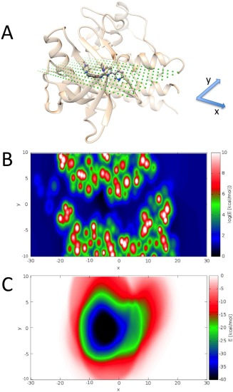
Comparison between the “actual” energy landscape of the protein and the attracting cavity landscape. A) Experimental structure of the Imatinib/c‐Kit complex (PDB44 ID 1T4665). C‐Kit is displayed as a beige ribbon and Imatinib in ball and stick representation. Green dots show the plane on which the “actual” or the attracting cavivity energy landscapes were calculated. (B) Log‐scale of the “actual” energy landscape of the protein. (C) Attracting cavity energy landscape, calculated as described in the Methods section for an aliphatic carbon atom with a charge of −0.09 e. The energy minimum corresponds to the center of the binding site. The attracting cavity energy landscape offers a smooth driving force for energy minimization, contrarily to the rough actual energy landscape. Heat maps were obtained using the gnuplot program (http://www.gnuplot.info).

Table 1 shows the success rate obtained by AC, using different sampling conditions and ligand initial conformations. When the AC approach uses the bioactive ligand conformer during the initial ligand positioning, the success rate for the top‐ranked binding mode in reproducing the X‐ray native binding mode ranges from 83.5% to 88.2%. Not surprisingly, the success rate is higher when the thoroughness of the sampling is increased by applying smaller rotation steps during the initial ligand positioning. In about 95% of the cases, the native binding mode was found within the five top‐ranked docking solutions. This illustrates the good performance of the scoring function, which is able to rank the native binding mode first in about 90% of the cases when the native binding mode is indeed present among the docking poses. Importantly, although starting from the experimental conformer provides an advantage for the sampling approach, this does not correspond to a rigid body ligand docking. Indeed, during the docking process, the ligand is prepositioned on the points of the attracting cloud, which unless by chance does not contain the geometrical center of the ligand in the experimental structure. In addition, the ligand is energy‐minimized during the docking and does not retain its bioactive conformation.

Table 1.

Success rate, in %, considering only the top‐ranked binding mode (Rank 1) or the 5 top‐ranked binding modes (Rank 5) and average CPU time for one docking run, in minutes, on a single Xeon E5440 2.83 GHz.

		Random conformer		X‐ray conformer
Software	Conditions	Rank1	Rank5	Rank1	Rank5	CPU Time (min)
Attracting Cavities	NThr =70 + 90 deg rot./(25 Å)3 box	81.2	90.6	84.7	95.3	134
	NThr =60 + 90 deg rot./(25 Å)3 box	75.3	89.4	83.5	94.1	210
	NThr =50 + 90 deg rot./(25 Å)3 box	74.1	83.5	83.5	92.9	360
	NThr =70 + 60 deg rot./(25 Å)3 box	83.5	91.8	84.7	94.1	460
	NThr =60 + 60 deg rot./(25 Å)3 box	77.7	87.1	87.1	96.5	730
	NThr =50 + 60 deg rot./(25 Å)3 box	81.2	91.8	87.1	95.3	1250
	NThr =70 + 45 deg rot./(25 Å)3 box	82.4	92.9	87.1	95.3	1000
	NThr =60 + 45 deg rot./(25 Å)3 box	81.2	91.8	88.2	94.1	1600
	NThr =50 + 45 deg rot./(25 Å)3 box	81.2	92.9	87.1	95.3	2650
Autodock Vina19	Exhaustivity = 8/(25 Å)3 box	62.3	74.1	76.5	90.6	4
	Exhaustivity = 100/(25 Å)3 box	65.9	77.7	80.0	91.8	35
	Exhaustivity = 1000/(25 Å)3 box	65.9	78.8	81.2	91.8	195
Autodock 4.215	run100; pop_size=150; num_evals=12,500,000/(25 Å)3 box	47.1	65.9	55.3	78.8	200
	run200; pop_size=150; num_evals=25,000,000/(25 Å)3 box	45.6	65.9	55.3	80.0	1050
ICM28	Search space is an orthorhombic box, extending 4 Å from the native binding mode in each direction. 10 runs.	9136	95 [a]36	NA	NA	NA
Surflex‐Dock53	??	6637	NA	NA	NA	NA
FRED54	??	7038	NA	NA	NA	NA
DOCK610	Search space is extending 8 Å from heavy atoms in native binding mode	70.339	NA	76.439	NA	NA
	Search space is extending 10 Å from heavy atoms in native binding mode	65.239	NA	NA	NA	NA
MOE Docker55	??	8040	NA	NA	NA	NA
Glide SP51, 52	Search space dimension = 14 + 0.8x (max separation of ligand atoms in Å)	8241	NA	NA	NA	NA
GOLD16	Search space defined as the residues with at least one heavy atom within 6 Å from the native binding mode of the ligand. Important water molecules kept.	8742	NA	NA	NA	NA
LEAD Finder56	Success if 10 runs within 2 Å out of 20.	74.143	NA	NA	NA	NA

A success is defined as the ability to reproduce the experimental binding mode of a protein‐ligand complex within 2 Å RMSD. For attracting cavities (AC), the N _Thr parameter determines the thoroughness of the AC sampling procedure; N _Thr=70 concentrates the sampling efforts on cavities, while N _Thr=50 samples the entire protein surface (see Methods). The rotation step of the initial ligand positioning procedure is also given, in degrees.

[a] Rank3 instead of Rank5.

??, no precise indication was given about the search space and the docking parameters in the literature; NA, not available.

When the memory effect of the ligand geometry is totally erased by recreating a 3D conformer with Open Babel from the ligand SMILES, i.e., from a 1D chemical structure notation, the success rate ranges from 74% to 84% for the top‐ranked docking solutions and 84% to 93% within the five top‐ranked docking solutions. The success of a docking is not determined by the differences between the native and the randomized conformations. Indeed, for the 69 docking successes obtained starting from a randomized conformation and using N _Thr = 50 and 45° rotation steps during the sampling, the RMSD calculated on the heavy atoms between the native and starting randomized conformers (RMSD_start) ranges from 0.07 to 3.71 Å (with a median RMSD_start of 1.6 Å). RMSD_start was larger than 2 Å for 17 ligands. For the 16 docking failures in the same conditions, RMSD_start ranges from 0.12 to 3.66 Å (with a median RMSD_start of 1.8 Å). RMSD_start was larger than 2 Å for 6 ligands. This indicates that, despite the absence of a specific dihedral optimization during the docking, the conformational sampling of the ligand provided by simple energy minimization in the AC environment is sufficient to generate native‐like conformations and binding modes in most cases, even when starting from remote conformers (Fig. 5A).

Figure 5.

Examples of docking success and failure. (A) Top: ligand conformation in the native binding mode (left) compared with the randomized conformation (right) for 1YWR66. The RMSD between the two conformations calculated on the heavy atoms after fitting is 3.7 Å. Bottom: comparison between the experimental binding mode (ball and stick) and the top‐ranked binding mode calculated with AC (cyan stick). The RMSD between the two binding modes is 1.0 Å, corresponding to a docking success. (B) Top: ligand conformation in the native binding mode (left) compared with the randomized conformation (right) for 1HVY67. The RMSD between the two conformations calculated on the heavy atoms after fitting is 3.2 Å. Bottom: comparison between the experimental binding mode (ball and stick) and the top‐ranked binding mode calculated with AC (cyan stick). The RMSD between the two binding modes is 2.8 Å, corresponding to a docking failure. [Color figure can be viewed in the online issue, which is available at wileyonlinelibrary.com.]

When a large rotation step is applied during the sampling (i.e., 90°, see Methods), a low value of N _Thr, which focuses the sampling in protein cavities, provides a higher success rate compared to larger N _Thr values, which extend the search on less concave regions. This is easily explained by the fact that most of the ligands in the Astex test set are buried in deep cavities: the limited sampling offered by a 90° rotation step is sufficient if the search is limited to well‐defined cavities, but somewhat insufficient if extended to the whole protein surface. When the sampling is strengthened by applying smaller rotation steps (i.e., 60° or 45°) high success rates are also obtained when the entire surface of the protein is included (N _Thr = 50). Therefore, a sound choice for N _Thr and the rotation steps enables the user saving time during the docking with AC by focusing the search in cavities if the ligand is known to be deeply buried or extending the search to the entire protein surface with equivalent efficiency otherwise.

We have chosen to validate the AC approach on the Astex diverse set31 of ligand‐protein complexes since several docking algorithms, i.e., ICM,28 Glide SP,51, 52 GOLD,16 Surflex‐Dock,53 FRED,54 DOCK6,10 MOE Docker,55 and LEAD Finder,56 were benchmarked on this test set in a recent series of concerted articles.36, 37, 38, 39, 40, 41, 42, 43

To complete the comparison, we also benchmarked AutoDock 4.2 and Autodock Vina, since they are currently the most‐cited free and open‐source docking programs.49, 50 For AutoDock and AutoDock Vina, the docking was performed using exactly the same starting conformations of the ligand and the same search space as for AC. Several values of the sampling parameters were used to test the performance of the programs in different conditions. Docking parameters and search spaces were different for the other software and are briefly mentioned in Table 1, when known. When starting from the bioactive conformer, the success rate of Autodock Vina ranges from 76.5% to 81.2% for the top‐ranked calculated binding modes, as a function of the search exhaustiveness, and from 90.6% to 91.8% when considering the five top‐ranked binding modes. These results are comparable to the 80% success rate recently published for the same benchmark set in similar conditions.57 When starting from a ligand conformation generated by Open Babel, the rank1 and rank5 success rates range from 62.3% to 65.9% and from 74.1% to 78.8%, respectively. Using large values for the sampling parameters, Autodock 4.2 success rate at rank1 and rank5 is around 55% and 80%, respectively, when starting from the bioactive conformer, and 47% and 66% when starting from a conformation generated by Open Babel. These results show the existence of a memory effect in the success rates of Autodock 4.2 and Autodock Vina regarding the ligand starting geometry, although these programs are generally considered to experience little or no such effect. We think that starting the docking from a ligand conformer generated by a chemoinformatics package, rather than just randomizing the dihedral angles as it is often done, provides a more realistic assessment of the program performance. Indeed, this process mimics real docking campaigns where the ligand geometry is usually generated by chemoinformatics programs with 1D or 2D chemical definitions as input. This procedure requires the docking program to also optimize the bond lengths, bond angles, and the conformation of nonaromatic cycles during the sampling process. Noticeably, the performance of Autodock Vina on this benchmark set depends little on the value of the exhaustiveness parameter.

Table 2 provides the number of sampling and scoring failures for each AC, Autodock 4.2, and Autodock Vina run. A run was considered a sampling failure when no docking pose within the five top‐ranked clusters has a RMSD from the X‐ray binding mode lower than 2 Å. We considered only the five top‐ranked clusters rather than the entire population of poses, since this would artificially favor AC, which can output many very diverse poses including the highest energy ones. If a run was not a sampling failure, it was considered a scoring failure if no docking pose with a RMSD from the X‐ray binding mode lower than 2 Å was ranked first. When starting from the bioactive conformer, the fraction of sampling and scoring failures of the different AC runs (from 3.5% to 7.1% and from 6.3% to 11.3%, respectively) are comparable yet somewhat lower than that of Autodock Vina (from 8.2% to 9.4% and from 11.5% to 15.6%, respectively) and significantly smaller than that of Autodock 4.2 (from 20.0% to 21.2% and from 29.9% to 30.9%, respectively). When starting from a random conformer, the fraction of sampling failures increases twofold for AC (from 7.1% to 16.5%), threefold for Autodock Vina (from 21.2% to 26.9%), and significantly for Autodock 4.2 (34.1%). The rate of scoring failures is unchanged for Autodock 4.2 and slightly higher for AC (from 9.0% to 11.3%, with one run at 15.8%) and for Autodock Vina (from 15.2% to 16.4%). Only nine test cases lead to 80% of AC sampling failures. These complexes are characterized by either direct contact between the ligand and a metal ion, Zn (1HQ2), or several water molecules bridging the ligand–protein interactions (1W1P, 1XOQ, 1MEH, 1SQ5, 1HVY, and 1N2J). These explicit water molecules were removed prior to the docking. Sampling failures occur systematically when starting from the random conformer in only two test cases: 1HVY and 1VCJ. Similarly, only nine test cases lead to 80% of the scoring failures. In four of them, i.e., 1P2Y, 1JD0, 1OQ5, and 1R1H, the ligand is interacting directly with a metal ion (Zn, or the Fe atom of a heme moiety). Other cases, i.e., 1N2J, 1GM8, 1G9V, 1HVY, and 1MEH, are characterized by a large number of ligand–protein interactions bridged by water molecules. The Astex test set contains one case where the ligand is in direct interaction with a heme Fe atom and two cases with a Mg atom, which all lead to docking failures. In 13 cases, where the ligand is in contact with a Zn atom, AC obtains a success rate of 70% (so lower compared with the entire Astex test set). This difficulty to predict binding modes in proteins with important metal atoms in the binding site is a known limitation of the scoring function employed here. This can be corrected using a morse‐like metal binding potential (MMBP)58 or a QM/MM rescoring.59 In summary, nearly all sampling and scoring failures of AC could be attributed to the presence of a metal ion in the binding site or the fact that numerous important water molecules were removed before the docking. In all other complexes tested, AC provided satisfactory results.

Table 2.

Sampling and scoring failures for each AC, Autodock Vina, and Autodock 4.2 run.

		Random conformer, n (%)		X‐ray conformer, n (%)
Software	Conditions	Samp. Fail.	Scor. Fail.	Samp. Fail.	Scor. Fail.
Attracting Cavities	NThr =70 + 90 deg rot.	8/85 (9.4)	6/77 (7.8)	4/85 (4.7)	9/81 (11.1)
	NThr =60 + 90 deg rot.	9/85 (10.6)	12/76 (15.8)	5/85 (5.9)	9/80 (11.3)
	NThr =50 + 90 deg rot.	14/85 (16.5)	8/71 (11.3)	6/85 (7.1)	8/79 (10.1)
	NThr =70 + 60 deg rot.	7/85 (8.2)	7/78 (9.0)	5/85 (5.9)	8/80 (10.0)
	NThr =60 + 60 deg rot.	11/85 (12.9)	8/74 (10.8)	3/85 (3.5)	8/82 (9.8)
	NThr =50 + 60 deg rot.	7/85 (8.2)	9/78 (11.5)	4/85 (4.7)	7/81 (8.6)
	NThr =70 + 45 deg rot.	6/85 (7.1)	10/79 (12.7)	4/85 (4.7)	7/81 (8.6)
	NThr =60 + 45 deg rot.	7/85 (8.2)	9/78 (11.5)	5/85 (5.9)	5/80 (6.3)
	NThr =50 + 45 deg rot.	6/85 (7.1)	10/79 (12.7)	4/85(4.7)	7/81 (8.6)
Autodock Vina19	Exhaustivity = 8	22/85 (26.9)	10/63 (15.9)	8/85 (9.4)	12/77 (15.6)
	Exhaustivity = 100	19/85 (22.4)	10/66 (15.2)	7/85 (8.2)	10/78 (12.8)
	Exhaustivity = 1000	18/85 (21.2)	11/67 (16.4)	7/85 (8.2)	9/78 (11.5)
Autodock 4.215	run100; pop_size=150; num_evals=12,500,000	29/85 (34.1)	16/56 (28.6)	18/85 (21.2)	20/67 (29.9)
	run200; pop_size=150; num_evals=25,000,000	29/85 (34.1)	17/56 (30.4)	17/85 (20.0)	21/68 (30.9)

In comparison, six test cases lead to systematic sampling failures with Autodock Vina, regardless of the starting conformation or sampling exhaustivity. They are characterized by the direct interaction of the ligand with a heme Fe atom (1P2Y) or several important water molecules in the active site (1G9V, 1SQ5, 1W1P, 1GM8, and 1HVY). They account for 40% of the sampling failures of Autodock Vina. However, 11 additional test cases lead to a systematic sampling error when starting from a random conformer, while leading to a docking success or a scoring failure when starting from the bioactive conformation: 1L2S, 1L7F, 1MMV, 1MZC, 1N2J, 1OWE, 1Q41, 1T46, 1U4D, 1YWR, and 2BM2. Fourteen test cases account for 90% of the scoring failures of Autodock Vina. Some are characterized by the direct interaction of the ligand with a Zn atom (1JD0, 1R55) or important water molecules in the active site (1MEH, 1UOU, 1N2V, and 1U4D). For other test cases (1YGC, 1IG3, 1L2S, 1GPK, 1Q1G, 1Q41, 1XM6, and 2BR1), the native pose was not ranked first, but its score was only 0.1 to 0.6 kcal/mol higher than the one of the top‐ranked pose. This could not be attributed to the absence of an important water molecule during the docking, the presence of a metal ion nor a crystal contact in the X‐ray structure and is, thus, likely to indicate some limitation of the scoring function, which is difficult to predict.

In its current implementation, AC is 30 to 50 times slower than Autodock Vina when the fastest sampling parameters are used for both programs (Table 1), making AC more suitable for a limited number of docking runs for which high precision is required, than for high‐throughput virtual screening.

In summary, AC compares well with AutoDock Vina and AutoDock 4.2 in reproducing the experimental binding modes of the Astex diverse set under similar conditions. AC also provides better results than Surflex‐Dock, FRED, DOCK, and LEAD Finder, despite the fact that, in some cases, these programs concentrated their effort on a smaller search space or identified the best prediction using another criterion than the best score. AC performance is comparable with that of MOE Docker and Glide SP. ICM outperformed all docking programs on this benchmark set, with a 91% success rate for the top‐ranked calculated binding mode; however, the search space is significantly smaller.

Although the success rate of AC on the Astex test set is satisfying, several improvements can be proposed. Currently, the ligand conformation is optimized only by simple energy minimizations. The reported results show that this is sufficient in most cases, but this procedure is sometimes unable to perform the large rearrangement between the starting conformation of the ligand provided by the user and the bioactive one (Fig. 5). Combining a dihedral optimization with the present algorithm should significantly enhance its performance to this regard. Several ways to increase the speed of AC will be investigated: a grid‐based evaluation of the ligand–protein interaction energy and a better consideration of the ligand and binding‐site shapes to filter the initial poses submitted to energy minimization. In addition, the use of the CHARMM force field and the CHARMM package to estimate ligand–protein interactions opens the way for including not only protein flexibility but also on‐the‐fly QM/MM docking.59

Conclusion

A new docking algorithm, called AC, was presented and tested. The idea behind AC is to replace the rough energy landscape of the protein by a smooth attractive energy landscape generated by virtual attracting points surrounding the protein surface. We demonstrated that simple energy minimizations in this smooth landscape, followed by additional minimizations in the actual protein energy landscape, become an efficient sampling algorithm for docking. The scoring function of AC is based on the CHARMM force field and the FACTS solvation model. The use of this universal scoring ensures the transferability of our results to other type of macromolecular targets (e.g., DNA) and to other type of ligands (e.g., molecular fragments).

AC uses a new simple algorithm to identify protein cavities, which allows fine‐tuning the sampling procedure to focus more on deep protein cavities or, on the contrary, to include less concave regions.

The approach was assessed on the 85 ligand–protein complexes of the Astex diverse set. AC achieved a success rate of about 80% in reproducing the experimental binding mode within 2Å RMSD, starting from a completely randomized ligand conformer. The algorithm thus compares favorably with current state‐of‐the‐art docking programs.

The realistic prediction of ligand–receptor binding geometries is an important task in SB‐CADD. It has been observed that consensus scoring, which consists in rescoring docking poses with several scoring functions, performs better in identifying the native binding mode than the best stand‐alone scoring algorithm.60, 61, 62 It has also been shown that combining scoring functions of different types (e.g., empirical and knowledge based) provides a better performance than combining scoring functions of similar types.63 More recently, Houston and Walkinshaw showed that consensus docking, i.e., combining different sampling algorithms and not only different scoring functions improves the reliability of docking in virtual screening.64 AC is of particular interest in the context of consensus docking since it is based on the combination of a unique sampling algorithm and a universal physics‐based scoring function.

How to cite this article: Zoete V., Schuepbach T., Bovigny C., Chaskar P., Daina A., Röhrig U. F., Michielin O.. J. Comput. Chem. 2016, 37, 437–447. DOI: 10.1002/jcc.24249

References

- 1. Sousa S. F., Ribeiro A. J. M., Coimbra J. T. S., Neves R. P. P., Martins S. A., Moorthy N. S. H. N., Fernandes P. A., Ramos M. J., Curr. Med. Chem., 2013, 20, 2296. [DOI] [PubMed] [Google Scholar]
- 2. Zoete V., Grosdidier A., Michielin O., J. Cell. Mol. Med. 2009, 13, 238 DOI:10.1111/j.1582-4934.2008.00665.x. [DOI] [PMC free article] [PubMed] [Google Scholar]
- 3. Grinter S. Z., Zou X., Molecules. 2014, 19, 10150 DOI:10.3390/molecules190710150. [DOI] [PMC free article] [PubMed] [Google Scholar]
- 4. Rarey M., Kramer B., Lengauer T., Klebe G., J. Mol. Biol. 1996, 261, 470 DOI:10.1006/jmbi.1996.0477. [DOI] [PubMed] [Google Scholar]
- 5. Claussen H., Buning C., Rarey M., Lengauer T., J. Mol. Biol. 2001, 308, 377. DOI:10.1006/jmbi.2001.4551. [DOI] [PubMed] [Google Scholar]
- 6. Grosdidier A., Zoete V., Michielin O., J. Comput. Chem. 2011, 32, 2149 DOI:10.1002/jcc.21797. [DOI] [PubMed] [Google Scholar]
- 7. Cecchini M., Kolb P., Majeux N., Caflisch A., J. Comput. Chem. 2004, 25, 412 DOI:10.1002/jcc.10384. [DOI] [PubMed] [Google Scholar]
- 8. Kuntz I. D., Blaney J. M., Oatley S. J., Langridge R., Ferrin T. E., J. Mol. Biol. 1982, 161, 269. [DOI] [PubMed] [Google Scholar]
- 9. Ewing T. A., Makino S., Skillman A. G., Kuntz I., J. Comput. Aided Mol. Des. 2001, 15, 411. [DOI] [PubMed] [Google Scholar]
- 10. Lang P. T., Brozell S. R., Mukherjee S., Pettersen E. F., Meng E. C., Thomas V., Rizzo R. C., Case D. A., James T. L., Kuntz I. D., RNA. 2009, 15, 1219 DOI:10.1261/rna.63609. [DOI] [PMC free article] [PubMed] [Google Scholar]
- 11. Welch W., Ruppert J., Jain A., Chem. Biol. 1996, 3, 449. [DOI] [PubMed] [Google Scholar]
- 12. Bohm H. J., J. Comput. Aided Mol. Des. 1992, 6, 593. [DOI] [PubMed] [Google Scholar]
- 13. Grosdidier A., Zoete V., Michielin O., Proteins. 2007, 67, 1010 DOI:10.1002/prot.21367. [DOI] [PubMed] [Google Scholar]
- 14. Grosdidier A., Zoete V., Michielin O., J. Comput. Chem. 2009, 30, 2021 DOI:10.1002/jcc.21202. [DOI] [PubMed] [Google Scholar]
- 15. Morris G. M., Huey R., Lindstrom W., Sanner M. F., Belew R. K., Goodsell D. S., Olson A. J.. J. Comput. Chem. 2009, 30, 2785 DOI:10.1002/jcc.21256. [DOI] [PMC free article] [PubMed] [Google Scholar]
- 16. Jones G., Willett P., Glen R. C., Leach A. R., Taylor R., J. Mol. Biol. 1997, 267, 727 DOI:10.1006/jmbi.1996.0897. [DOI] [PubMed] [Google Scholar]
- 17. Verdonk M. L., Cole J. C., Hartshorn M. J., Murray C. W., Taylor R. D., Proteins. 2003, 52, 609 DOI:10.1002/prot.10465. [DOI] [PubMed] [Google Scholar]
- 18. McMartin C., Bohacek R., J. Comput. Aided Mol. Des., 1997, 11, 333. [DOI] [PubMed] [Google Scholar]
- 19. Trott O., Olson A. J., J. Comput. Chem. 2010, 31, 455 DOI:10.1002/jcc.21334. [DOI] [PMC free article] [PubMed] [Google Scholar]
- 20. Totrov M., Abagyan R., Proteins. 1997, 1, 215. [DOI] [PubMed] [Google Scholar]
- 21. Liu M., Wang S., J. Comput. Aided Mol. Des., 1999, 13, 435. [DOI] [PubMed] [Google Scholar]
- 22. Liu Y., Zhao L., Li W., Zhao D., Song M., Yang Y., J. Comput. Chem. 2012, 34, 67 DOI:10.1002/jcc.23108. [DOI] [PubMed] [Google Scholar]
- 23. Chen H. M., Liu B. F., Huang H. L., Hwang S. F., Ho S. Y., J. Comput. Chem. 2007, 28, 467 DOI:10.1002/jcc.20542. [DOI] [PubMed] [Google Scholar]
- 24. Namasivayam V., Günther R., Chem. Biol. Drug Des. 2007, 70, 475 DOI:10.1111/j.1747-0285.2007.00588.x. [DOI] [PubMed] [Google Scholar]
- 25. Meier R., Pippel M., Brandt F., Sippl W., Baldauf C., J. Chem. Inf. Model. 2010, 50, 879 DOI:10.1021/ci900467x. [DOI] [PubMed] [Google Scholar]
- 26. Sousa S. F., Fernandes P. A., Ramos M. J., Proteins. 2006, 65, 15 DOI:10.1002/prot.21082. [DOI] [PubMed] [Google Scholar]
- 27. Luitz M. P., Zacharias M., J. Chem. Inf. Model. 2014, 54, 1669 DOI:10.1021/ci500296f. [DOI] [PubMed] [Google Scholar]
- 28. Abagyan R., Totrov M., Kuznetsov D., J. Comput. Chem. 1994, 15, 488 DOI:10.1002/jcc.540150503. [Google Scholar]
- 29. Brooks B. R., Brooks C. L., Mackerell A. D., Nilsson L., Petrella R. J., Roux B., Won Y., Archontis G., Bartels C., Boresch S., Caflisch A., Caves L., Cui Q., Dinner A. R., Feig M., Fischer S., Gao J., Hodoscek M., Im W., Kuczera K., Lazaridis T., Ma J., Ovchinnikov V., Paci E., Pastor R. W., Post C. B., Pu J. Z., Schaefer M., Tidor B., Venable R. M., Woodcock H. L., Wu X., Yang W., York D. M., Karplus M., J. Comput. Chem. 2009, 30, 1545 DOI:10.1002/jcc.21287. [DOI] [PMC free article] [PubMed] [Google Scholar]
- 30. Haberthür U., Caflisch A., J. Comput. Chem. 2008, 29, 701 DOI:10.1002/jcc.20832. [DOI] [PubMed] [Google Scholar]
- 31. Hartshorn M. J., Verdonk M. L., Chessari G., Brewerton S. C., Mooij W. T. M., Mortenson P. N., Murray C. W., J. Med. Chem. 2007, 50, 726 DOI:10.1021/jm061277y. [DOI] [PubMed] [Google Scholar]
- 32. Zoete V., Cuendet M. A., Grosdidier A., Michielin O., J. Comput. Chem. 2011, 32, 2359 DOI:10.1002/jcc.21816. [DOI] [PubMed] [Google Scholar]
- 33. Zoete V., Grosdidier A., Cuendet M., Michielin O., J. Mol. Recognit. 2010, 23, 457 DOI:10.1002/jmr.1012. [DOI] [PubMed] [Google Scholar]
- 34. Roche O., Kiyama R., Brooks C. L., J. Med. Chem. 2001, 44, 3592. [DOI] [PubMed] [Google Scholar]
- 35. MacKerell A. D., Bashford D., Bellott, Dunbrack R. L., Evanseck J. D., Field M. J., Fischer S., Gao J., Guo H., Ha S., Joseph‐McCarthy D., Kuchnir L., Kuczera K., Lau F. T. K., Mattos C., Michnick S., Ngo T., Nguyen D. T., Prodhom B., Reiher W. E., Roux B., Schlenkrich M., Smith J. C., Stote R., Straub J., Watanabe M., Wirkiewicz‐Kuczera J., Yin D., Karplus M., J. Phys. Chem. B, 1998, 102, 3586. [DOI] [PubMed] [Google Scholar]
- 36. Neves M. A. C., Totrov M., Abagyan R., J. Comput. Aided Mol. Des. 2012, 26, 675 DOI:10.1007/s10822-012-9547-0. [DOI] [PMC free article] [PubMed] [Google Scholar]
- 37. Spitzer R., Jain A. N., J. Comput. Aided Mol. Des. 2012, 26, 687 DOI:10.1007/s10822-011-9533-y. [DOI] [PMC free article] [PubMed] [Google Scholar]
- 38. McGann M., J. Comput. Aided Mol. Des. 2012, 26, 897 DOI:10.1007/s10822-012-9584-8. [DOI] [PubMed] [Google Scholar]
- 39. Brozell S. R., Mukherjee S., Balius T. E., Roe D. R., Case D. A., Rizzo R. C., J. Comput. Aided Mol. Des. 2012, 26, 749 DOI:10.1007/s10822-012-9565-y. [DOI] [PMC free article] [PubMed] [Google Scholar]
- 40. Corbeil C. R., Williams C. I., Labute P., J. Comput. Aided Mol. Des., 2012, 26, 775 DOI:10.1007/s10822-012-9570-1. [DOI] [PMC free article] [PubMed] [Google Scholar]
- 41. Repasky M. P., Murphy R. B., Banks J. L., Greenwood J. R., Tubert‐Brohman I., Bhat S., Friesner R. A., J. Comput. Aided Mol. Des. 2012, 26, 787 DOI:10.1007/s10822-012-9575-9. [DOI] [PubMed] [Google Scholar]
- 42. Liebeschuetz J. W., Cole J. C., Korb O., J. Comput. Aided Mol. Des., 2012, 26, 737 DOI:10.1007/s10822-012-9551-4. [DOI] [PubMed] [Google Scholar]
- 43. Novikov F. N., Stroylov V. S., Zeifman A. A., Stroganov O. V., Kulkov V., Chilov G. G., J. Comput. Aided Mol. Des. 2012, 26, 725 DOI:10.1007/s10822-012-9549-y. [DOI] [PubMed] [Google Scholar]
- 44. Berman H. M., Nucleic Acids Res. 2000, 28, 235 DOI:10.1093/nar/28.1.235. [DOI] [PMC free article] [PubMed] [Google Scholar]
- 45. Pettersen E. F., Goddard T. D., Huang C. C., Couch G. S., Greenblatt D. M., Meng E. C., Ferrin T. E., J Comput Chem 2004, 25, 1605 DOI:10.1002/jcc.20084. [DOI] [PubMed] [Google Scholar]
- 46. Dunbrack R. L., Curr. Opin. Struct. Biol., 2002, 12, 431. [DOI] [PubMed] [Google Scholar]
- 47. Brünger A. T., Karplus M., Proteins 1988, 4, 148 DOI:10.1002/prot.340040208. [DOI] [PubMed] [Google Scholar]
- 48. O'Boyle N. M., Banck M., James C. A., Morley C., Vandermeersch T., Hutchison G. R., J. Cheminform. 2011, 3, 33 DOI:10.1093/nar/gkp324. [DOI] [PMC free article] [PubMed] [Google Scholar]
- 49. Yuriev E., Agostino M., Ramsland P. A., J. Mol. Recognit., 2011, 24, 149 DOI:10.1002/jmr.1077. [DOI] [PubMed] [Google Scholar]
- 50. Yuriev E., Ramsland P. A., J. Mol. Recognit., 2013, 26, 21, 79. DOI:10.1002/jmr.26. [DOI] [PubMed] [Google Scholar]
- 51. Friesner R., Banks J., Murphy R., Halgren T., Klicic J., Mainz D., Repasky M., Knoll E., Shelley M., Perry J., Shaw D., Francis P., Shenkin P., J. Med. Chem. 2004, 47, 1739 DOI:10.1021/jm0306430. [DOI] [PubMed] [Google Scholar]
- 52. Halgren T., Murphy R., Friesner R., Beard H., Frye L., Pollard W., Banks J., J. Med. Chem. 2004, 47, 1750 DOI:10.1021/jm030644s. [DOI] [PubMed] [Google Scholar]
- 53. Jain A. N., J. Comput. Aided Mol. Des. 2007, 21, 281 DOI:10.1007/s10822-007-9114-2. [DOI] [PubMed] [Google Scholar]
- 54. Warren G. L., Andrews C. W., Capelli A. M., Clarke B., LaLonde J., Lambert M. H., Lindvall M., Nevins N., Semus S. F., Senger S., Tedesco G., Wall I. D., Woolven J. M., Peishoff C. E., Head M. S., J. Med. Chem., 2006, 49, 5912 DOI:10.1021/jm050362n. [DOI] [PubMed] [Google Scholar]
- 55. Molecular Operating Environment (MOE). Chemical Computing Group, Montreal, Quebec, Canada, 2011.
- 56. Stroganov O. V., Novikov F. N., Stroylov V. S., Kulkov V., Chilov G. G., J. Chem. Inf. Model. 2008, 48, 2371 DOI:10.1021/ci800166p. [DOI] [PubMed] [Google Scholar]
- 57. Ruiz‐Carmona S., Alvarez‐Garcia D., Foloppe N., Garmendia‐Doval A. B., Juhos S., Schmidtke P., Barril X., Hubbard R. E., Morley S. D., PLoS Comput. Biol. 2014, 10, e1003571 DOI:10.1371/journal.pcbi.1003571. [DOI] [PMC free article] [PubMed] [Google Scholar]
- 58. Röhrig U. F., Grosdidier A., Zoete V., Michielin O., J. Comput. Chem. 2009, 30, 2165 DOI:10.1002/jcc.21244. [DOI] [PubMed] [Google Scholar]
- 59. Chaskar P., Zoete V., Röhrig U. F., J Chem Inf Model 2014, 54, 3137 DOI:10.1021/ci5004152. [DOI] [PubMed] [Google Scholar]
- 60. Charifson P. S., Corkery J. J., Murcko M. A., Walters W. P., J. Med. Chem. 1999, 42, 5100 DOI:10.1021/jm990352k. [DOI] [PubMed] [Google Scholar]
- 61. Guo J., Hurley M. M., Wright J. B., Lushington G. H., J. Med. Chem. 2004, 47, 5492 DOI:10.1021/jm049695v. [DOI] [PubMed] [Google Scholar]
- 62. Stahl M., Rarey M., J. Med. Chem. 2001, 44, 1035 DOI:10.1021/jm0003992. [DOI] [PubMed] [Google Scholar]
- 63. Cheng T., Li X., Li Y., Liu Z., Wang R., J. Chem. Inf. Model. 2009, 49, 1079 DOI:10.1021/ci9000053. [DOI] [PubMed] [Google Scholar]
- 64. Houston D. R., Walkinshaw M. D., J. Chem. Inf. Model. 2013, 53, 384 DOI:10.1021/ci300399w. [DOI] [PubMed] [Google Scholar]
- 65. Mol C. D., Dougan D. R., Schneider T. R., Skene R. J., Kraus M. L., Scheibe D. N., Snell G. P., Zou H., Sang B. C., Wilson K. P., J. Biol. Chem. 2004, 279, 31665 DOI:10.1074/jbc.M403319200. [DOI] [PubMed] [Google Scholar]
- 66. Golebiowski A., Townes J. A., Laufersweiler M. J., Brugel T. A., Clark M. P., Clark C. M., Djung J. F., Laughlin S. K., Sabat M. P., Bookland R. G., VanRens J. C., De B., Hsieh L. C., Janusz M. J., Walter R. L., Webster M. E., Mekel M. J., Bioorg. Med. Chem. Lett. 2005, 15, 2285 DOI:10.1016/j.bmcl.2005.03.007. [DOI] [PubMed] [Google Scholar]
- 67. Phan J., Koli S., Minor W., Dunlap R. B., Berger S. H., Lebioda L., Biochemistry. 2001, 40, 1897 DOI:10.1021/bi002413i. [DOI] [PubMed] [Google Scholar]