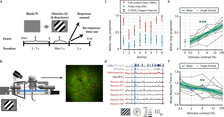
Figure 1. Mice perform a go/no-go task during in vivo calcium imaging.

(a) Task schematic showing the time course of a single trial. In each trial, one of a combination of eight different directions and five contrasts, or a 0% contrast probe trial (isoluminant gray blank screen) was presented (ratio 1:5 of 0%-contrast-probe:stimulus trials). When mice made a licking response during stimulus presentation, the visual stimulus was turned off and sugar water was presented. (b) Schematic of experimental setup. During task performance, we recorded eye movements with an infrared-sensitive camera, licking responses, and running on a treadmill. (c) All eight animals performed statistically significant stimulus detection during neural recordings, as quantified by non-overlapping 2.5th–97.5th Clopper–Pearson (CP) percentile confidence intervals (95% CI) (p<0.05) of behavioral response proportions for 0% and 100% contrast probe trials. (d) Example of simultaneously recorded behavioral measures, population heterogeneity, mean population dF/F₀, and traces of neurons labeled in panel (b) Vertical colored bars represent stimulus presentations; width, color, and saturation represent duration, orientation, and contrast, respectively. (e, f) Animals showed significant increases in behavioral response (behav. resp.) proportion (linear regression analysis, see ‘Materials and methods’, p<0.001) (e) and reductions in reaction time (p<0.01); (f) with higher stimulus contrasts. Shaded areas show the standard error of the mean. Statistical significance: **p<0.01; ***p<0.001.

DOI: http://dx.doi.org/10.7554/eLife.10163.003

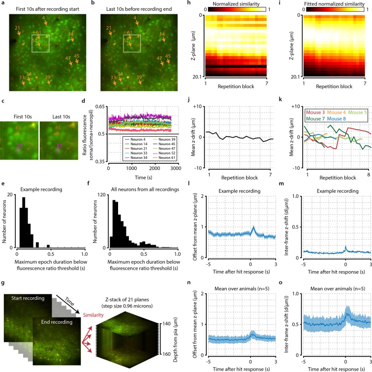
Figure 1—figure supplement 1. Neuronal signals are stable over time.

(a, b) Example from one animal showing the average of all recorded frames during the first 10 s after imaging onset (a) and during the last 10 s before the end of the recording (b). The locations of 10 randomly selected neurons are marked by orange arrows, and the white-colored rectangles depict the area enlarged in panel (c). (c) Enlarged subsection of the images shown in (a) and (b) showing the outlines of cells 52 and 61. Note the similarity of the cell bodies and their outlines. (d) Down-sampled traces showing the ratio of soma versus neuropil fluorescence of the 10 randomly selected neurons shown in panels (a) and (b) over duration of the entire recording (see ‘Materials and methods’). All traces remain above the equiluminance threshold of 0.5, indicating that these neurons’ somata remain visible and do not disappear due to bleaching or slow z-drift. (e) Histogram showing the maximum epoch duration of dropping below the equiluminance threshold of 0.5 for all neurons from the example session of (a–d). None of the cells remain undetectable for longer than 0.5 s. (f) as (e) but for all cells from all recordings. None of the cells have a prolonged period (>1.0 s) of being undetectable, indicating stability of the neuronal signals over time. (g) Schematic showing procedure of z-drift calculation for example animal. For each repetition block of 48 trials, we compared the similarity of 100 frames (~4 s) in the beginning, middle, and end of each stimulus repetition set to slices recorded at different cortical depths (step size 0.96 µm). (h) Similarity values normalized between [0-1] for each time point show a small and slow z-drift over the entirety of the recording. (i) To quantify this drift, we fitted each time point with a Gaussian. (j) The mean of the fitted Gaussian shows that maximum drift in z-direction for this animal did not exceed 4 µm. (k) Data for all animals of which we recorded z-stacks (n=5/8). Animals 2 (not shown) and 7 showed excessive z-drift, so we split their recordings into two populations (see ‘Materials and methods’). Within a single recorded population, z-drift never exceeded 8 µm for any animal. (l–o) Frame-by-frame analysis of fast z-shifts during entire recordings show that z movement rarely exceeds more than a couple of microns. (l) Example recording showing mean ± standard error across trials in offset from mean z-plane as a function of time after hit response (licking). Shortly after the behavioral response, a peak in variability can be observed. However, note that for all analyses we only included epochs before the licking response; the period of neural responses with potential contamination from z-shifts will, therefore, not influence our results. (m) Example frame-by-frame shift in microns (mean ± standard error across trials) shows a similar time course as the mean z-offset. (n, o) Same as panels (l) and (m), but showing mean ± standard error across animals (n=5).

DOI: http://dx.doi.org/10.7554/eLife.10163.004