Ozone Trends and their Relationship to Characteristic Weather Patterns

Abstract

Background

Local trends in ozone concentration may differ by meteorological conditions. Furthermore, the trends occurring at the extremes of the Ozone distribution are often not reported even though these may be very different than the trend observed at the mean or median and they may be more relevant to health outcomes.

Aims

Classify days of observation over a 16 year period into broad categories that capture salient daily local weather characteristics. Determine the rate of change in mean and median O₃ concentrations within these different categories to assess how concentration trends are impacted by daily weather. Further examine if trends vary for observations in the extremes of the O₃ distribution.

Methods

We used k-means clustering to categorize days of observation based on the maximum daily temperature, standard deviation of daily temperature, mean daily ground level wind speed, mean daily water vapor pressure and mean daily sea-level barometric pressure. The five cluster solution was determined to be the appropriate one based on cluster diagnostics and cluster interpretability. Trends in cluster frequency and pollution trends within clusters were modeled using Poisson regression with penalized splines as well as quantile regression.

Results

There were five characteristic groupings identified. The frequency of days with large standard deviations in hourly temperature decreased over the observation period, whereas the frequency of warmer days with smaller deviations in temperature increased. O₃ trends were significantly different within the different weather groupings. Furthermore, the rate of O₃ change for the 95^th percentile and 5^th percentile was significantly different than the rate of change of the median for several of the weather categories.

Conclusions

We found that O₃ trends vary between different characteristic local weather patterns. O₃ trends were significantly different between the different weather groupings suggesting an important interaction between changes in prevailing weather conditions and O₃ concentration.

1. INTRODUCTION

Regulations and technological improvements implemented over the past decades have caused marked improvement in air quality over many areas in the United States. In particular, pollutant trends over the Northeastern United States have been shown to be decreasing for many important pollutants including PM_2.5, NO₂, SO₂ and CO (1–3). Trends for median O₃ concentrations have a more mixed result, with some studies suggesting decreases while others suggest no significant trends (4–7). There is also evidence that background O₃ concentrations have been increasing, perhaps due to an increase in conditions that are favorable to O₃ formation such as higher temperature and shifts in the NOx/VOC ratio (5,8,9). A good understanding of the factors driving long-term changes in O₃ concentration is crucial in order to better inform policy decisions.

The strong seasonal patterns in ambient O₃ concentrations have been well described worldwide as well as in the North Eastern United States (10,11). The seasonality in O₃ concentrations is related both to the effects of meteorological conditions on rates of O₃ formation as well as to changes in the availability of precursors. The meteorological factors relating to O₃ formation are intensity of solar radiation, cloud cover, temperature, water vapor pressure and boundary layer height. Changes in prevailing wind directions exhibit seasonal dependence and also determine the sources and concentrations of transported O₃ precursors (12).

Local spring-time ozone maxima have been observed at many remote locations, thought to be less impacted by anthropogenic emissions (13,14). Two-main processes are thought to contribute to these spring time maxima. These are Stratosphere-troposphere exchange (STE) of O₃ rich stratospheric air into the troposphere as well as increases in solar-radiation acting on O₃ precursors that have accumulated over the winter period (15). Profound STE events resulting in significant O₃ intrusion into the troposphere are generally associated with extreme weather events, such as thunderstorms which can be identified through local weather variables such as local wind speed, water vapor pressure, barometric pressure and fluctuations in ground-level temperatures (16). Stagnation, which generally occurs in the North-Eastern United States in the height of summer, is characterized by low wind speed and high ambient temperature, leads to extremely favorable conditions for O₃ formation (17).

Concentrations of anthropogenic O₃ precursors show a strong seasonal dependence as well. The decomposition rate of peroxyacetylinitrate (PAN), an important sink for both NO_x and radicals, is highly dependent on ambient temperature (18). Isoprene emissions from plants, a major VOC precursor to O₃, have also been shown to be highly temperature dependent (19). Lastly, NO_x concentrations are generally higher in winter because the reduced oxidative capacity of the atmosphere results in longer residence time. Since these important precursors are strongly influenced by temperature, this is yet another important facet of the complex relationship between temperature and O₃ formation.

Larger time-scale changes in weather may also have an impact on O₃ concentrations. Over the past 3 decades, clear trends in weather conditions, including extreme temperature events, total precipitation and humidity have been observed (20,21). Furthermore, changes in synoptic weather patterns, such as changes in the strength of the North Atlantic Oscillation, El Niño–Southern Oscillation, as well as changes in the frequency of the Mid-Latitude Cyclone may contribute to altering concentrations of transported air pollutants over New England (22,23).

Considering weather conditions when performing trend analysis for O₃ is therefore crucial. Commonly, temperature and wind speed are accounted for as a main effect in the regression model used to calculate trend (24). Including a wider range of meteorological variables in a regression model can be problematic due to issues of correlation between weather variables. Different approaches have been used to resolve this problem including smoothing over a larger spatial area (25), neural network models (26), cluster analysis and classification tree approaches (27,28) and probabilistic models (29).

In order to better understand how trends in air pollution are impacted by short- and long-term scale changes in climate we propose to classify days of observation in a 16 year period based on the multivariate relationship between local weather variables. Within each of these identified groups, we will perform a trend analysis of O₃ over the time period. This approach allows us to identify how the O₃ concentrations are changing independently of long-term changes in local weather patterns. Differences in trends within each weather pattern group will also be examined for quantiles of the O₃ distribution. Observed differences in trend can then be ascribed to changes that are independent of weather patterns such as changes in emissions of VOC and NO_x precursors to O₃ formation.

2. METHODS

The different steps undertaken in this methods section are summarized in Figure 1.

Figure 1.

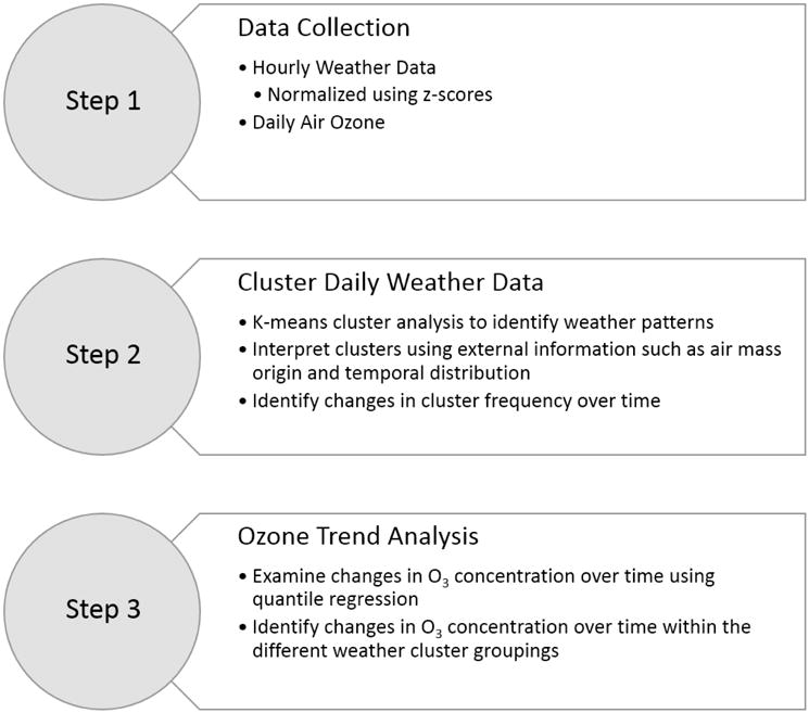
Methods summary chart

2.1 Data

The weather data used in this study included hourly measurements recorded at the Boston Logan airport as provided by the National Oceanic and Atmospheric Administration (NOAA) database. The data used were collected during 1995–2010 and 24-hour averages were estimated for days with at least 75% completeness in the hourly data. From 1995–2010, O₃ data measured at 4 sites within the metropolitan Boston, MA, area were obtained from the US EPA’s aerometric information retrieval system. We computed city wide averages to better capture regional distribution. Although the focus of this paper is the ozone trends, concentrations of NO₂, NO_x, SO₂ and BC were also retrieved from US EPA’s aerometric information retrieval system to aid interpretation of the results. Trend analysis for these pollutants was performed, in order to compare with the O₃ results.

The weather variables used in the cluster analysis included maximum daily temperature, standard deviation of daily temperature, mean daily ground level wind speed, mean daily water vapor pressure (absolute water content of the air), and mean daily sea-level pressure. These weather variables are used to characterize different physical properties thus their distributions and units are different. For this reason their values were converted to z-scores which were used for clustering. There were 87 days excluded from the analysis due to more than 25% missing hourly data.

2.2 Clustering

Clusters were identified using k-means cluster analysis, Hartigan-Wong algorithm (30). We allowed for values of k (number of clusters) to range between 2 and 10. To ensure that the solution selected is stable and not a local minimum, the k-means algorithm was run 1,000 times with 1,000 different random initial seeds. The solution with the lowest sum of squares within (SSW) was retained as the best solution for the given conditions. The large number of initial seed values helped to ensure that the solution did not correspond to a local minimum (31). For all values of k, the algorithm converged within 300 iterations.

The number of clusters (k) was selected using three main criteria. The first was the desire to pick a solution that yielded a reasonable total SSW value (keeping in mind that SSW decreases as the number of clusters decreases). The second was a desire to minimize pollutant concentration variability within the clusters of a given solution and the third was to identify clusters that were interpretable based on our knowledge of weather patterns in the Boston area.

The k-means algorithm used was implemented in the kmeans function of the stats package in R v. 2.15.2.

2.3 Comparing Clustering Solutions

The Rand Index is a measure of similarity between two different partitions of the same data set. This indexranges between 0 and 1 where 0 indicates that two data clusters do not agree on any pair of points and 1 indicating that the data clusters are exactly the same. The Rand Index represents a weight of the sites classified together in the two solutions versus the sites classified separately. In this paper, we used the adjusted Rand Index in order to compare different clustering solutions. First proposed by (32) the adjusted Rand Index corrects the Rand Index for the random chance that pairs are classified together. Steinley et al. (2004) suggested that an adjusted Rand Index greater than 0.9 reflected excellent agreement, values greater than 0.8 reflected good agreement, values greater than 0.65 indicated moderate agreement and less than 0.65 indicated poor agreement (33).

2.4 Back-Trajectory Analysis

Back-trajectory paths were calculated using the HYSPLIT model (v. 4.9) developed by National Oceanic and Atmospheric Administration (NOAA). The meteorological archive used was the Eta Data Assimilation System with 40 km resolution (EDAS40). For every hour of every day from 2004 to 2009, an 84 hour back-trajectory was computed in HYSPLIT from the starting coordinates of the sampling site and a vertical height of 750 m. The vertical movement of air parcels within the system was modeled using an isentropic assumption (34–36). Unfortunately, because the EDAS40 data begins in 2004, it was not possible to obtain earlier back-trajectory information in the same projection space.

The back-trajectory information begins in 2004 as this was the first year available at this higher grid resolution. We use these data as a representative sample of our data set which ranges from 1995–2010. This approach is also supported by the sensitivity analysis which shows no great changes in the clustering results over the early and later parts of the study period as discussed below.

2.5 Trend analysis

Trend analysis of yearly cluster frequency was performed using both a generalized additive Poisson model with a penalized spline term representing the year, in order to allow for non-linear trends. The penalized spline was calculated using the MGCV package in R v. 2.15.2.

O₃ trends were described using a linear regression model, controlling for seasonality using sine and cosine functions and day of week as an indicator variable. In addition, a quantile regression model was used to model differences in trends for different quantiles of O₃ concentrations over time. This model also controlled for seasonality with sine and cosine functions as well as day of week using an indicator variable. Quantile regression was first proposed by Koenker (1978) as a robust alternative to traditionally used mean estimator (37). In addition, quantile regression allows us to estimate the trend for different quantiles in the data, allowing us to observe changes in the extremes of the dataset, e.g., trends in baseline pollution and regional smog episodes. Quantile regression was performed using the quantreg package in R v. 2.15.2.

3. RESULTS

3.1 Selecting k

We selected the number of clusters (k) to be 5. Figure 2 (a) shows the fractional change in SSW for increases in k from 2 to 10. As k increases the value of the SSW decreases; however, the decrease slows significantly after k=5. In part this justifies selecting 5 as the number of clusters.

Figure 2.

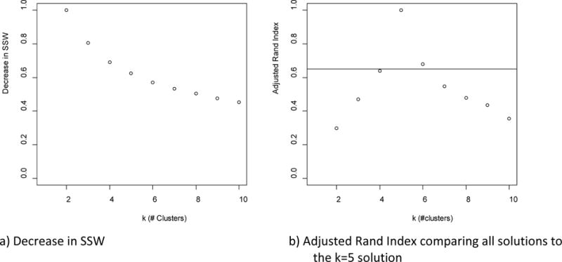
Selecting the number of clusters (k)

We also considered the 4 and 6 cluster solution. However, the 5 cluster solution proved to be more interpretable based on general knowledge of weather patterns throughout the Boston year. The 5 cluster solution showed a clear seasonal pattern which was a goal when we were seeking to partition this data.

3.2 Cluster Descriptions

The clusters were sorted based on the number of days per cluster, from largest to smallest. Important meteorological and chemical characteristics of each cluster are presented in Table 1. The monthly distribution of each cluster is presented in Figure 3 (a). Interpretation of the clusters is based on their mean characteristics.

Table 1.

Summary of the 5 clusters (bolded rows represent variables used in clustering)

	Cluster 1 – 1523 Days Winter Low Boundary Layer	Cluster 2 – 1308 Days Summer Moderate Weather	Cluster 3 – 1145 Days Winter High Boundary Layer	Cluster 4 – 946 Days Summer Regional Pollution Event	Cluster 5 – 834 Days Transition High SD of Temp.
	Mean (SD)	Mean (SD)	Mean (SD)	Mean (SD)	Mean (SD)
Temp (C)	2 (5)	16 (4)	4 (6)	23 (3)	13 (6)
max T past 3 days (C)	7 (6)	21 (6)	9 (7)	26 (4)	16 (7)
max T today (C) SD Hourly Temp (C)	6 (5)       2 (1)	19 (4)       2 (1)	8 (6)       2 (1)	29 (3)       3 (1)	20 (6)       4 (1)
(mbar)	5 (2)	14 (4)	6 (3)	20 (4)	9 (3)
Sea-Level Pressure (mbar)	1022 (6)	1016 (6)	1007 (7)	1013 (5)	1017 (7)
Ozone (ppb)	18 (9)	22 (9)	24 (9)	35 (12)	27 (11)
8-hour max ozone (ppb)	26 (10)	32 (11)	31 (9)	52 (17)	39 (14)
Wind Speed (m/s)	5 (1)	4 (1)	7 (2)	5 (1)	5 (1)
Boundary Layer Height (m)	686 (329)	620 (226)	1086 (399)	785 (224)	801 (312)
PM2.5 (ug/m3)	10 (5)	10 (5)	7 (4)	16 (9)	10 (5)
Sulfur Dioxide (ppb)	7 (4)	3 (2)	4 (3)	3 (2)	4 (3)
Nitrogen Dioxide (ppb)	23 (7)	19 (6)	17 (6)	19 (7)	21 (8)
Nitrogen Monoxide (ppb)	24 (20)	15 (11)	12 (8)	9 (6)	16 (12)
Black Carbon (ug/m3)	0.9 (0.6)	1.0 (0.6)	0.6 (0.4)	1.1 (0.6)	0.9 (0.6)
Precipitation per day (mm)	1 (5)	3 (10)	6 (12)	2 (7)	1 (4)

Figure 3.

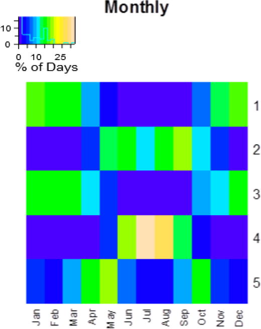
Distribution of clusters

Clusters 1 and 3 occur primarily in the winter months. Cluster 1 is characterized by high sea-level pressure and low boundary layer height, whereas cluster 3 is characterized by lower sea-level pressure, higher precipitation and higher boundary layer. Cluster 1 is higher in NO and BC whereas cluster 3 is higher in O₃. The higher concentration of primary pollutants in cluster 1 may be reflective of decreased mixing on those days due to a lower boundary height.

Clusters 2 and 4 are primarily in warm weather clusters. Cluster 4 occurred in June, July and August whereas cluster 2 was more spread out in time from May until October. The mean daily temperature of cluster 4 is 23 °C, as compared to 16 °C for cluster 2, and the water vapor pressure is significantly higher in cluster 4. The meteorological conditions occurring in Cluster 4 are consistent with summer time regional pollution events due to photochemical transformation of pollutants. This is confirmed by the elevated PM_2.5 and O₃ concentrations as well as very high maximum 8-hr O₃ and the low NO concentrations in cluster 4.

Cluster 5 occurs in the transition months (spring and fall) and is characterized by moderate temperatures (13 °C) and moderate O₃ and PM_2.5. In addition, the standard deviation of the hourly temperature values is highest in Cluster 5 than other clusters suggesting strong diurnal temperature differences.

In order to determine the persistence of different clusters, we calculated the number of consecutive days belonging to the same cluster (cluster runs). Figure 3 (b) shows that the median number of consecutive days ranges between 1 and 2. There are infrequent episodes that occur where consecutive days can be as high as 16. Cluster 5 seems to have the fewest such consecutive days.

3.3 Wind Directions

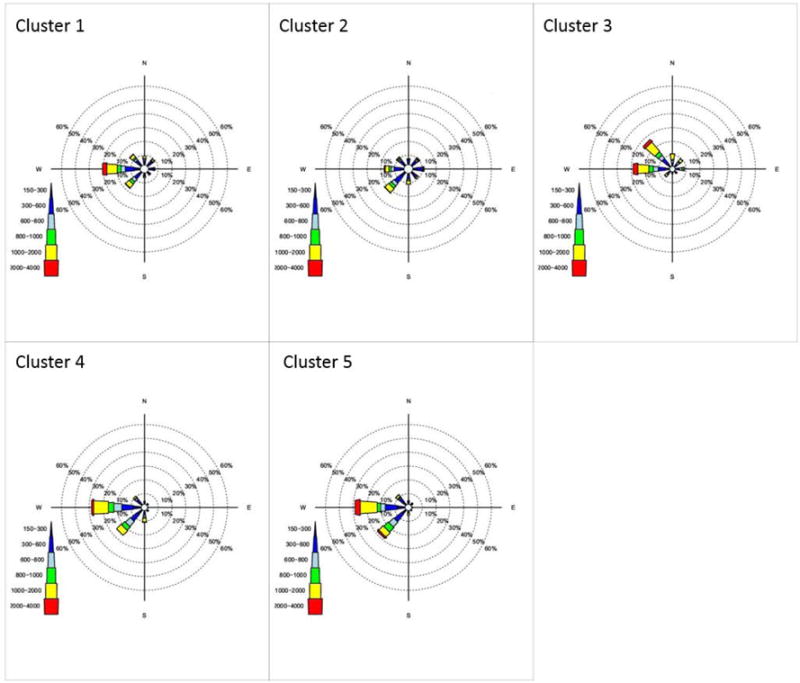
Ground-level hourly wind direction measurements were available for every day of observation. We compared the percent of hours within 8 direction quadrants for each cluster. Figure 4 shows the results of this analysis. In cluster 1, 45% of the ground level wind directions were from the N-W quadrant. For cluster 2, 22% of the hourly wind directions were from the NE-E direction. Cluster 3 had 55% of the ground wind coming from the SW-NW direction. Cluster 4 had 60% of the wind coming from the S-W direction and cluster 5 had ground level wind directions ranging from S to NW. Because ground level wind direction does not necessarily indicate the direction of the prevailing winds, and potentially the origin of transported pollutants, we also wanted to plot hourly back-trajectories for the days in our observation period.

Figure 4.

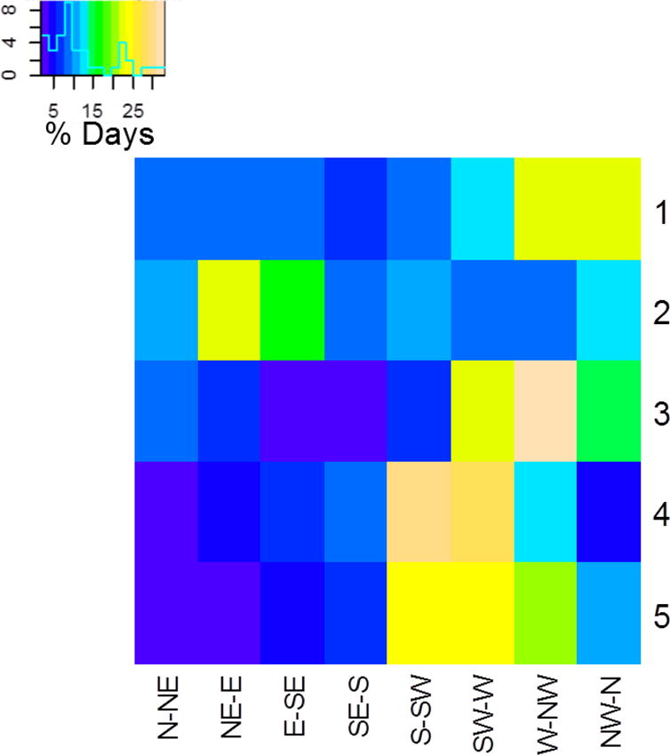
Percent of observed hours within each direction bin by cluster

Figure 5 shows the distance and location from Boston of all the hourly back-trajectories that were less than 1,500 meters above ground level in the 72 hours prior to arriving in Boston. The visualization was done with the heR.misc package (38). This figure further demonstrates the differences between clusters that were observed in the same season. The winter clusters have very different profiles with cluster 3 (associated with high boundary layer height) showing a significant contribution of air masses from the NW. The summer clusters also have very different profiles with Cluster 4 (regional pollution) showing a strong contribution from air masses to the West of Boston that is not seen in Cluster 2. The transition season cluster has similar patterns of back-trajectories as Cluster 4 (regional pollution).

Figure 5.

Back-trajectory analysis 0–72 hours prior to sampling day and 0m–1000m from ground level.

3.4 Sensitivity Analysis

For the cluster analysis, we wanted to determine the sensitivity of the solution to the initial conditions. Firstly, we determined how sensitive the solution was to the number of clusters selected. As shown in Figure (b), the 4 and 6 cluster solution moderately agrees with the 5 cluster solution, whereas for other k values, the cluster solution is significantly different and less interpretable.

We also confirmed that clustering the data from the beginning of the observation period and the end of the observation period would not produce significantly different results. For this analysis, the dataset was separated into two parts, one with dates prior to 1/1/2003 and the second with dates starting at 1/1/2003. The two datasets were clustered into 5 clusters as described above. These two solutions were compared to the initial clustering that was obtained using the entire dataset. Comparing the early and late datasets to the solution obtained from all the years combined shows excellent comparability (adjusted Rand index of 0.95 and 0.88, respectively). Therefore, we conclude that it is appropriate to cluster and interpret the data over the entire observation period.

We examined how sensitive the solution was to missing days of observation in the data set. We randomly removed 10% of the days (576 days) to create 100 new datasets. We then clustered these 100 datasets and compared the results to our solution using the adjusted Rand index. The mean adjusted Rand index across all the datasets is 0.97 (sd=0.06).

3.5 Trend in yearly weather patterns

A trend analysis of the yearly frequency of each cluster as a function of the year of observation was performed. The use of a penalized spline to model the trend allows for non-linear relationships. The results are presented in Figure 6. There are no clear trends for clusters 1, 3 and 4. However, there is strong evidence that there is a linear decrease in the frequency of cluster 5 (1.3% per year) which corresponds to transition days and a linear increase in the frequency of cluster 2 (1 % per year) which corresponds to mild summer days.

Figure 6.

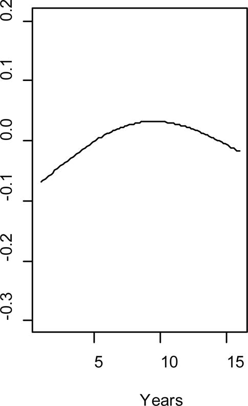
Trend in cluster frequency over time

3.6 Pollutant Trends

First, we examined the overall trend in concentrations of O₃, NO₂, SO₂, BC and PM_2.5 over the entire observation period without accounting for cluster groupings (Figure 7) using both linear regression and quantile regression. We further examined the differences in the trends for O₃ by cluster. The results for O₃ are presented in Figure 8. The trend values and standard errors are presented in Table 2. There are important differences in the trends both across clusters as well as across quantiles for the same cluster. Across all the clusters, the background concentrations of O₃ are increasing over time, although the magnitude of this difference is much smaller for Cluster 4 than the other clusters. The trends in the 95^th percentile values of O₃ are quite different over the different clusters. Cluster 4 has the strongest decline in the 95^th percentile value of O₃ (−0.69 ppb/year) whereas Cluster 5 has the strongest increase in the 95^th percentile value of O₃ (0.42 ppb/year). The differences in trend by cluster were also examined for the other pollutants, but there were no significant trend differences by cluster, results are not presented here.

Figure 7.

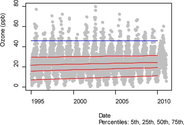
Quantile regression and linear regression of O₃, NO₂, SO₂, BC and PM_2.5 by year

Figure 8.

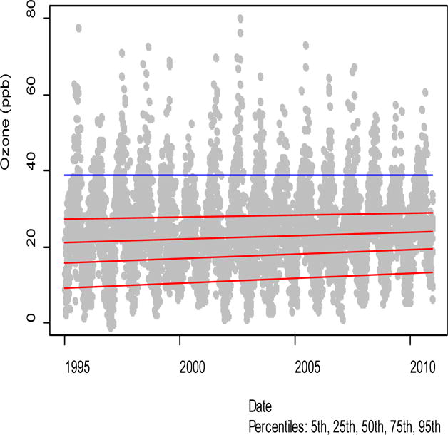
Trend analysis of Ozone by Cluster

Table 2.

Rate of change of Ozone from 1999–2010

	Cluster 1		Cluster 2		Cluster 3		Cluster 4		Cluster 5		Overall
Quantile	Change per year (ppb/year)	Standard Error	Change per year (ppb/year)	Standard Error	Change per year (ppb/year)	Standard Error	Change per year (ppb/year)	Standard Error	Change per year (ppb/year)	Standard Error	Change per year (ppb/year)	Standard Error
0.05	0.36	0.07	0.38	0.07	0.31	0.11	0.10	0.11	0.24	0.10	0.27	0.03
0.25	0.28	0.05	0.25	0.05	0.26	0.07	−0.02	0.11	0.21	0.06	0.24	0.03
0.5	0.30	0.04	0.23	0.05	0.09	0.05	−0.06	0.10	0.11	0.08	0.18	0.03
0.75	0.28	0.04	0.11	0.07	0.07	0.05	−0.28	0.12	0.18	0.08	0.11	0.03
0.95	0.23	0.07	−0.08	0.10	−0.15	0.08	−0.69	0.25	0.42	0.14	0.02	0.05

Grey entries are not statistically different than 0 (p>=0.05)

In order to better understand the relative impact of changes in weather frequency vs changes in concentration within weather cluster, we calculated the change in O₃ concentration attributable to each process, over the 16 years of observation, as shown in Equation 1.

$$d[O_3]={\displaystyle \sum \{\frac{d{D}_i}{365d}\ast \overline{{[O_3]}_i}\ast 16y+d{[O_3]}_i\ast \frac{{\overline{D}}_i}{365d}\}}$$ Equation 1

Where

• d[O₃] is the change in O₃ over 16 years

• dD_i is the change in the number of days in cluster i over 16 years

• $\overline{{[O_3]}_i}$ is the median concentration of O₃ within cluster i

• d[O₃]_i is the change in concentration of O₃ within cluster i over the 16 year period

• $\frac{{\overline{D}}_i}{365d}$ is the average number of days (per year) belonging to cluster i

Results of this analysis are presented in Table 3. In general, the change in yearly concentration attributable to change in concentration within cluster is much higher than changes in concentration attributable to changes in yearly frequency. In addition, we can see that the change in trend for the baseline is much higher than for the median. The 95^th percentile concentration of O₃ is decreasing overall, but this is mainly due to important decreases in the 95^th concentration trend of Cluster 4. We also observe that clusters 1 and 2 are both strongly contributing to the overall increasing trend in O₃ concentration throughout the year. This analysis is instructive in contrasting how changes in weather and changes in rates of formation of O₃ are driving the overall differences being observed.

Table 3.

The change in O₃ (ppb) attributable to changes in cluster frequency and changes in concentration within cluster over the 16 year period of observation

Change in MEDIAN O3 (ppb) over the 16 year period
	Cluster 1	Cluster 2	Cluster 3	Cluster 4	Cluster 5	OVERALL CHANGE
Due to Δ Frequency	0.23	0.66	−0.06	−0.23	−0.86	−0.26
Due to Δ Concentration	1.30	0.88	0.36	−0.01	0.23	2.76
TOTAL	1.53	1.54	0.30	−0.24	−0.63	2.51

Change in 5th Percentile O3 (ppb) over the 16 year period
	Cluster 1	Cluster 2	Cluster 3	Cluster 4	Cluster 5	OVERALL CHANGE
Due to Δ Frequency	0.07	0.26	−0.03	−0.12	−0.32	−0.13
Due to Δ Concentration	1.36	0.98	1.05	0.20	0.45	4.04
TOTAL	1.43	1.24	1.03	0.08	0.13	3.91

Change in 95th Percentile O3 (ppb) over the 16 year period
	Cluster 1	Cluster 2	Cluster 3	Cluster 4	Cluster 5	OVERALL CHANGE
Due to Δ Frequency	0.46	1.14	−0.10	−0.38	−1.43	−0.31
Due to Δ Concentration	1.03	−0.39	−0.34	−1.79	0.44	−1.05
TOTAL	1.49	0.75	−0.44	−2.17	−0.99	−1.36

We determined that including categorical values for month instead of describing seasonality as a periodic function did not significantly affect the trend estimates. We also examined whether the assumption of linearity in the trends of O₃ was reasonable by also modeling the trends using basis splines. There was no evidence of strong deviation from linearity.

4. DISCUSSION

The weather clusters identified represent 5 main daily weather types that occur in the Boston area. These categories are based on the maximum daily temperature, standard deviation of the daily temperature, ground level wind speed, water vapor pressure, and the sea level pressure. Examining the trends in O₃ concentration within each of these characteristic meteorological groupings allows for a better understanding of the trend of O₃ over time, independent of trends in climate and changes in the duration and start of seasonal conditions. Furthermore, our results demonstrate that modeling mean O₃ values does not provide adequate information on O₃ trends at the extremes. This has been previously demonstrated in other instances (39). The overall trend in baseline O₃ (0.27 ± 0.07 ppb/year) as determined by the quantile regression of the 5^th percentile in O₃ concentration over the time-period agrees with those of other studies reporting trends in O₃ baseline over the West Coast of Ireland, (0.31 ± 0.12 ppb/year) (40) and off the West Coast of the USA, 0.5–0.8 ppb/year (9).

We know that weather strongly influences O₃ formation and removal. Examining the trend in O₃ concentrations within the 5 identified clusters allows for the investigation of the relationship changes in O₃ concentrations independent of changes in weather patterns. Over the 16 year time-period, the sensitivity analysis confirmed that the cluster types did not change significantly rather there has been a clear change in the yearly frequency of the clusters over time. There was a decrease in the frequency of cluster 5 (1.3% per year) and an increase in the frequency of cluster 2 (1 % per year). Cluster 2 corresponds to warmer days in the summer with higher nighttime temperatures, while cluster 5 corresponds to days in the transition seasons with lower nighttime temperatures and mild daytime temperatures. Therefore, we have observed a decrease in transition season days and an increase of days with summer characteristics in the spring and fall seasons. Furthermore, cluster 2 corresponds to days with Easterly winds. Although 16 years of data is a short time to make any inference about long-term changes in temperature trends, this observation does coincide with climate change studies that note a decrease in the daily standard deviation of temperature being recorded during the winter and transition seasons in the northeast (41,42).

Classifying based on daily weather allows for important trends to be observed. In particular, baseline concentrations on stagnant summer days remain unchanged. By contrast, baseline concentration in mild summer conditions are increasing more rapidly than dataset as a whole (0.38 ± 0.14 ppb/year). Winter clusters also show strong increases in baseline O₃ concentrations. The high boundary layer winter days (Cluster 3) show slight decreases (−0.15 ± 0.14 ppb/year) in upper quantiles of O₃. These days are characterized by low pressure, air masses from the NW and high precipitations. The decrease in maximum O₃ concentrations is possibly due to increases in winter precipitation over the NE that have been observed in climate change studies (43). Winter days with low boundary layer height show an increase of 0.23 ± 0.13 ppb/year in the 95^th percentile. These days are associated with low precipitation and higher concentrations of primary pollutants, including NO. The increase in the 95^th percentile concentrations of O₃ may indicate that over time on these days, O₃ formation is increasingly limited by NO_x concentrations. Ozone concentration on transition season days have increases in the 95^th percentile at a rate of 0.42 ± 0.26 ppb/year. This agrees with observations of recent increases in spring maxima O₃ concentrations (13). Significant decrease in O₃ in the upper quantiles of Cluster 4 (−0.70 ± 0.55 ppb/year) agrees with previous evidence that effective emission controls have decreased summertime smog episodes over NE North America (3).

Comparing this clustering method to examining O₃ trends by season demonstrates the added value in categorizing days based on observed weather patterns rather than by fixed seasonal time periods. Figure 9 shows the results of the trend analysis of O₃ by season. The increase in transition season maxima is not at all visible with this analysis method. Furthermore, differences between low and high pressure days are also not evident. The decrease in higher quantile values in the stagnant summer conditions is captured however, perhaps because these days tend to be highly concentrated within the summer months. The magnitude of the decrease in trend is decreased as compared to the clustering method. We also performed a second analysis which additionally controlled for daily temperature as well as season and observed no significant differences between this model and the model that only accounted for season.

Figure 9.

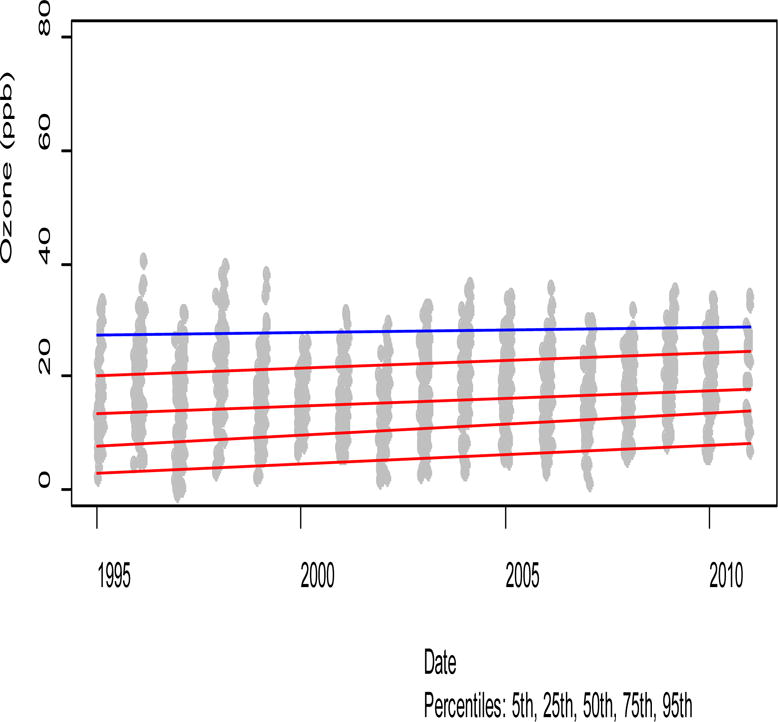
Trends in O₃ by Season

The results of the trends in frequency and the trends in O₃ concentration within cluster were combined in order to assess their respective contributions on total O₃ concentration (Table 3). The overall change in O₃ concentration is strongly driven by changes occurring within clusters 1 and 2. Both these clusters have markedly low mixing heights as compared to the other clusters. In addition, they both have significantly higher concentrations of NO. The increase in O₃ observed here appears to be associated with photochemistry of locally emitted pollutants as opposed to regional transported pollutants.

In addition, the results of Table 3 suggest that there is an overall increase in the 95^th percentile of O₃ in the transition weather group. This trend is particularly concerning given recent analyses suggest increased susceptibility to air pollution in the spring time. Within 10 Canadian cities, springtime weather was associated with a stronger response to O₃ among the elderly. In addition, they observed higher RR estimates in the springtime (44). Likewise, stronger associations between air pollution and mortality and morbidity have been observed in the springtime (45,46).

For comparison we estimated the trends of other pollutants. The trends of NO_x, SO₂, BC and PM_2.5 in this time period are shown in. For these four pollutants, the quantile regression results indicate a stronger decrease for the higher percentile values than for the low level values, indicating that background concentrations are not changing as quickly as the higher concentrations. This suggests that emission controls are having a positive impact on high ground level concentrations. Although not shown here, there is no observable difference in the trends of these pollutants by cluster, suggesting that the trends in these pollutants are not weather dependent.

Because the NO_x/VOC ratio is an important factor in the rate of formation of O₃ we wanted to investigate whether the differences observed for the different weather clusters are related weather dependent trends in this ratio. When accounting for daily NO_x concentration in the trend analysis, the trends for clusters 1, 2, 3 and 5 become insignificant or marginally positive. On the other hand, the trends of O₃ within cluster 4 remain consistent with those observed when not accounting for NO_x. This suggests that other than in stagnant summer conditions, cluster specific changes in O₃ were associated with similar decreases in NO_x. This is due to the reaction of ozone with NO. This mechanism is more important during the winter and the night when the atmosphere is more stable and the local primary emissions containing NO have more impact on the transported ozone. However, this mechanism becomes less important during the summer episodes when ozone formation is enhanced and there is more vertical mixing.

5. Conclusions

The method presented here groups days of observation into meaningful and interpretable groupings that reflect characteristic weather patterns. These groupings can then be used to examine changes in O₃ concentrations over time. Seasonal analysis has been successfully used to identify differences in pollutant trends as well as differences in response to air pollution. However, this method allows for greater precision in identifying the exact calendar days that represent a cohesive weather grouping. The use of quantile regression allows for the identification of important trends that are occurring at the extremes of the distribution and that may be missed in a mean regression. These changes that are occurring at the extremes can be extremely important and yield information that is relevant to policy and decision making. The analysis demonstrates the effectiveness of emission control policies to diminish maximum summertime O₃ concentrations. However, it also demonstrates that baseline O₃ concentrations are significantly increasing, particularly in winter and moderate summer conditions. Furthermore, there is evidence that there is the need for increased O₃ controls in the transition months in order to curb the rising trend in maximum values.

References

- 1.Kelly VR, Lovett GM, Weathers KC, Likens GE. Trends in atmospheric concentration and deposition compared to regional and local pollutant emissions at a rural site in southeastern New York, USA. Atmos Environ. 2002;36(10):1569–1575. [Google Scholar]
- 2.Fann N, Risley D. The public health context for PM2. 5 and ozone air quality trends. Air Quality, Atmosphere & Health. 2013;6(1):1–11. [Google Scholar]
- 3.Parrish DD, Singh HB, Molina L, Madronich S. Air quality progress in North American megacities: a review. Atmos Environ. 2011;45(39):7015–7025. [Google Scholar]
- 4.Lin CC, Jacob DJ, Fiore AM. Trends in exceedances of the ozone air quality standard in the continental United States, 1980–1998. Atmos Environ. 2001;35(19):3217–3228. [Google Scholar]
- 5.Cooper O, Parrish D, Stohl A, Trainer M, Nédélec P, Thouret V, et al. Increasing springtime ozone mixing ratios in the free troposphere over western North America. Nature. 2010;463(7279):344–348. doi: 10.1038/nature08708. [DOI] [PubMed] [Google Scholar]
- 6.Bojkov RD, Bishop L, Fioletov VE. Total ozone trends from quality-controlled ground-based data (1964–1994) Journal of Geophysical Research: Atmospheres (1984–2012) 1995;100(D12):25867–25876. [Google Scholar]
- 7.Logan J, Staehelin J, Megretskaia I, Cammas J, Thouret V, Claude H, et al. Changes in ozone over Europe: Analysis of ozone measurements from sondes, regular aircraft (MOZAIC) and alpine surface sites. Journal of Geophysical Research: Atmospheres (1984–2012) 2012;117(D9) [Google Scholar]
- 8.Chan E, Vet R. Baseline levels and trends of ground level ozone in Canada and the United States. Atmospheric Chemistry & Physics. 2010;10:8629–8647. [Google Scholar]
- 9.Jaffe D, Ray J. Increase in surface ozone at rural sites in the western US. Atmos Environ. 2007;41(26):5452–5463. [Google Scholar]
- 10.Bloomer BJ, Vinnikov KY, Dickerson RR. Changes in seasonal and diurnal cycles of ozone and temperature in the eastern US. Atmos Environ. 2010;44(21):2543–2551. [Google Scholar]
- 11.Logan JA. Tropospheric ozone: Seasonal behavior, trends, and anthropogenic influence. Journal of Geophysical Research: Atmospheres (1984–2012) 1985;90(D6):10463–10482. [Google Scholar]
- 12.Schichtel BA, Husar RB. Eastern North American transport climatology during high-and low-ozone days. Atmos Environ. 2001;35(6):1029–1038. [Google Scholar]
- 13.Monks PS. A review of the observations and origins of the spring ozone maximum. Atmos Environ. 2000;34(21):3545–3561. [Google Scholar]
- 14.Allen DJ, Dibb JE, Ridley B, Pickering KE, Talbot RW. An estimate of the stratospheric contribution to springtime tropospheric ozone maxima using TOPSE measurements and beryllium-7 simulations. Journal of geophysical research. 2003;108(D4):8355. [Google Scholar]
- 15.Vingarzan R. A review of surface ozone background levels and trends. Atmos Environ. 2004;38(21):3431–3442. [Google Scholar]
- 16.Stohl A, Bonasoni P, Cristofanelli P, Collins W, Feichter J, Frank A, et al. Stratosphere-troposphere exchange: A review, and what we have learned from STACCATO. Journal of Geophysical Research: Atmospheres (1984–2012) 2003;108(D12) [Google Scholar]
- 17.Banta RM, Senff CJ, White AB, Trainer M, McNider RT, Valente RJ, et al. Daytime buildup and nighttime transport of urban ozone in the boundary layer during a stagnation episode. Journal of geophysical research. 1998;103(D17):22519–22,544. [Google Scholar]
- 18.Sillman S, Samson PJ. Impact of temperature on oxidant photochemistry in urban, polluted rural and remote environments. Journal of Geophysical Research: Atmospheres (1984–2012) 1995;100(D6):11497–11508. [Google Scholar]
- 19.Petron G, Harley P, Greenberg J, Guenther A. Seasonal temperature variations influence isoprene emission. Geophys Res Lett. 2001;28(9):1707–1710. [Google Scholar]
- 20.Peterson TC, Zhang X, Brunet-India M, Vázquez-Aguirre JL. Changes in North American extremes derived from daily weather data. Journal of Geophysical Research. 2008;113(D7):D07113. [Google Scholar]
- 21.Simmons A, Willett K, Jones P, Thorne P, Dee D. Low-frequency variations in surface atmospheric humidity, temperature, and precipitation: Inferences from reanalyses and monthly gridded observational data sets. Journal of Geophysical Research: Atmospheres (1984–2012) 2010;115(D1) [Google Scholar]
- 22.Leibensperger EM, Mickley LJ, Jacob DJ. Sensitivity of US air quality to mid-latitude cyclone frequency and implications of 1980–2006 climate change. Atmospheric Chemistry and Physics. 2008;8(23):7075–7086. [Google Scholar]
- 23.Doherty R, Stevenson D, Johnson C, Collins W, Sanderson M. Tropospheric ozone and El Niño–Southern Oscillation: Influence of atmospheric dynamics, biomass burning emissions, and future climate change. Journal of geophysical research. 2006;111(D19):D19304. [Google Scholar]
- 24.Lou Thompson M, Reynolds J, Cox LH, Guttorp P, Sampson PD. A review of statistical methods for the meteorological adjustment of tropospheric ozone. Atmos Environ. 2001;35(3):617–630. [Google Scholar]
- 25.Tai A, Mickley L, Jacob D, Leibensperger E, Zhang L, Fisher J, et al. Meteorological modes of variability for fine particulate matter (PM2. 5) air quality in the United States: implications for PM2. 5 sensitivity to climate change. Atmos Chem Phys. 2012;12:3131–3145. [Google Scholar]
- 26.Hooyberghs J, Mensink C, Dumont G, Fierens F, Brasseur O. A neural network forecast for daily average PM10 concentrations in Belgium. Atmos Environ. 2005;39(18):3279–3289. [Google Scholar]
- 27.Davis J, Eder B, Nychka D, Yang Q. Modeling the effects of meteorology on ozone in Houston using cluster analysis and generalized additive models. Atmos Environ. 1998;32(14–15):2505–2520. [Google Scholar]
- 28.Huang L, Smith RL. Meteorologically-dependent trends in urban ozone. Environmetrics. 1999;10(1):103–118. [Google Scholar]
- 29.Cox WM, Chu S. Meteorologically adjusted ozone trends in urban areas: a probabilistic approach. Atmospheric Environment.Part B.Urban Atmosphere. 1993;27(4):425–434. [Google Scholar]
- 30.Hartigan J, Wong M. A k-means clustering algorithm. Journal of the Royal Statistical Society C. 1979;28(1):100–108. [Google Scholar]
- 31.Steinley D. K-means clustering: A half-century synthesis. Br J Math Stat Psychol. 2006;59(1):1–34. doi: 10.1348/000711005X48266. [DOI] [PubMed] [Google Scholar]
- 32.Hubert L, Arabie P. Comparing partitions. Journal of classification. 1985;2(1):193–218. [Google Scholar]
- 33.Steinley D. Properties of the Hubert-Arable Adjusted Rand Index. Psychological Methods; Psychological Methods. 2004;9(3):386. doi: 10.1037/1082-989X.9.3.386. [DOI] [PubMed] [Google Scholar]
- 34.Draxler R, Rolph G. HYSPLIT (HYbrid Single-Particle Lagrangian Integrated Trajectory) model access via NOAA ARL READY. NOAA Air Resources Laboratory; Silver Spring: 2003. website ( http://www.arl.noaa.gov/ready/hysplit4.html) [Google Scholar]
- 35.Rolph GD, Draxler RR. Sensitivity of Three-Dimensional Trajectories to the Spatial and Temporal Densities of the Wind Field. J Appl Meteorol. 1990;29:1043–1054. [Google Scholar]
- 36.Rolph G. Real-time Environmental Applications and Display sYstem (READY) NOAA Air Resources Laboratory, Silver Spring; Silver Spring, MD: 2003. Website ( http://www.arl.noaa.gov/ready/hysplit4.html) [Google Scholar]
- 37.Koenker R, Bassett G., Jr Regression quantiles. Econometrica: journal of the Econometric Society. 1978:33–50. [Google Scholar]
- 38.Klepeis NE. The Human Exposure Research Software Package (heR) 2004 [Google Scholar]
- 39.Bradley RS, Griffiths ML. Variations of twentieth-century temperature and precipitation extreme indicators in the northeast United States. J Clim. 2007;20(21):5401–5417. [Google Scholar]
- 40.Brown PJ, Bradley RS, Keimig FT. Changes in Extreme Climate Indices for the Northeastern United States, 1870–2005. J Clim. 2010;23(24):6555–6572. [Google Scholar]
- 41.Vanos JK, Cakmak S, Bristow C, Brion V, Tremblay N, Martin SL, et al. Synoptic weather typing applied to air pollution mortality among the elderly in 10 Canadian cities. Environ Res. 2013 doi: 10.1016/j.envres.2013.08.003. [DOI] [PubMed] [Google Scholar]
- 42.Zanobetti A, Schwartz J. The Effect of Fine and Coarse Particulate Air Pollution on Mortality: A National Analysis. Environ Health Perspect. 2009 Jun;117(6):898–903. doi: 10.1289/ehp.0800108. [DOI] [PMC free article] [PubMed] [Google Scholar]
- 43.Franklin M, Schwartz J. The impact of secondary particles on the association between ambient ozone and mortality. Environ Health Perspect. 2008;116(4):453. doi: 10.1289/ehp.10777. [DOI] [PMC free article] [PubMed] [Google Scholar]