Occupational Exposure to PM_2.5 and Incidence of Ischemic Heart Disease

Supplemental Digital Content is available in the text.

Abstract

Background:

We investigated the incidence of ischemic heart disease (IHD) in relation to accumulated exposure to particulate matter (PM) in a cohort of aluminum workers. We adjusted for time varying confounding characteristic of the healthy worker survivor effect, using a recently introduced method for the estimation of causal target parameters.

Methods:

Applying longitudinal targeted minimum loss-based estimation, we estimated the difference in marginal cumulative risk of IHD in the cohort comparing counterfactual outcomes if always exposed above to always exposed below a PM_2.5 exposure cut-off. Analyses were stratified by sub-cohort employed in either smelters or fabrication facilities. We selected two exposure cut-offs a priori, at the median and 10th percentile in each sub-cohort.

Results:

In smelters, the estimated IHD risk difference after 15 years of accumulating PM_2.5 exposure during follow-up was 2.9% (0.6%, 5.1%) using the 10th percentile cut-off of 0.10 mg/m³. For fabrication workers, the difference was 2.5% (0.8%, 4.1%) at the 10th percentile of 0.06 mg/m³. Using the median exposure cut-off, results were similar in direction but smaller in size. We present marginal incidence curves describing the cumulative risk of IHD over the course of follow-up for each sub-cohort under each intervention regimen.

Conclusions:

The accumulation of exposure to PM_2.5 appears to result in higher risks of IHD in both aluminum smelter and fabrication workers. This represents the first longitudinal application of targeted minimum loss-based estimation, a method for generating doubly robust semi-parametric efficient substitution estimators of causal parameters, in the fields of occupational and environmental epidemiology.

Studies of the health effects of occupational exposures can be misleading due to time-varying confounding, a component of the healthy worker survivor effect.^1,2 Robins and colleagues^3,4 have developed methods, known as G-methods, designed to generate unbiased estimates in the presence of time-varying confounders on the causal pathway. Although developed in the mid-1980s and applied in other settings,^5,6 it was not until recently that methodologies, such as the parametric G formula,⁸ inverse probability weighting of marginal structural models,⁹ and G-estimation of accelerated failure time models,¹⁰ were applied to address this problem in occupational studies.

These methods adjust for time-varying confounding by building prediction models for either the exposure assignment or the disease outcome. An alternative approach is to model both processes, giving the investigator two opportunities to correct for the time-varying confounding. Such methods are known as doubly robust, referring to the fact that they provide unbiased results if either of the two processes are modeled correctly.¹¹ Longitudinal targeted minimum loss-based estimation (TMLE)¹² is a more recently developed G-method which provides a doubly robust substitution estimator that allows for flexible modeling of selected likelihood components.^13,14

Particulate matter (PM) with an aerodynamic diameter of less than 2.5 μm (PM_2.5) is recognized as a major contributor to the global burden of heart disease, with the strongest evidence for direct cigarette smoke and air pollution sources.^15,16 We apply longitudinal TMLE to estimate the incidence of ischemic heart disease (IHD) under hypothetical interventions on accumulated exposure to PM_2.5 in a large population of actively employed aluminum manufacturing workers. Earlier research on heart disease in this cohort^17,18 demonstrated a positive association between IHD incidence and current exposure to PM_2.5 using both conventional survival methods and inverse weighted marginal structural models.

Unlike most occupational cohorts,¹⁹ time-varying information on personal characteristics, such as cigarette smoking, body mass index (BMI), as well as measures of underlying cardiovascular health were available for this study. Variables on the causal pathway between exposure at an earlier time period and heart disease can serve as confounders of the effect of accumulated exposure on risk of heart disease.²⁰ Workers with better health tend to accrue more exposure through the preferential movement of workers with worse health to both lower exposed jobs as well as out of the work force.^1,2 If poorer health was caused by prior exposure, standard statistical methods will not generate consistent estimates of the effect of accumulated exposure.²¹ We therefore investigated the relation between accumulated exposure to PM_2.5 and IHD using longitudinal TMLE in this dataset in an attempt to estimate the causal effect of exposure absent the biasing influence of the healthy worker survivor effect.

METHODS

The Study Population and Outcome

Hourly workers employed at one of 11 US aluminum smelters and fabrication facilities for more than 2 years between January 1, 1996, and December 31, 2012, who were also enrolled in the company health plan, were eligible for inclusion in the analysis. Before 2003, we assumed that all employed workers were enrolled in the company health plan; 97% of them filed a claim during this period. After 2003, when the company changed providers, active worker rolls were checked against an eligibility roster to determine enrollment. Eligible workers, regardless of hire date, were followed for incidence of IHD after a 2-year washout period, implemented to remove prevalent cases of heart disease from the cohort. Follow-up for each worker began at the later of January 1, 1998, or 2 years after hire and ended at termination of employment.

Workers were assigned to the smelter or fabrication sub-cohorts if they had ever held a job in the respective facility types. The analysis was stratified due to differences in composition and level of PM_2.5 between the two. Incident IHD was defined by any of the following events: (1) insurance billing claim for a indicative procedure, such as revascularization, angioplasty, or a bypass, (2) face-to-face visit with a provider with a relevant International Classification of Diseases (ICD) diagnosis code, (3) hospitalization for more than 2 days with the relevant ICD admitting code, or (4) matching record of death from the National Death Index with a relevant cause of death.

All research protocols were approved by the Office for the Protection of Human Subjects at the University of California at Berkeley.

Exposure Assessment

The details of the exposure assessment have been previously described by Noth et al.²² Each job was associated with a time-invariant exposure level to total particulate matter (TPM) based upon 8,385 personal samples collected by the company at 11 facilities between 1980 and 2011. Within eight of the facilities, additional samples were collected by our research team to determine the %PM_2.5 in the TPM. The %PM_2.5 was then multiplied by the TPM estimate to determine the mean concentration of PM_2.5 associated with a particular job. Additional modeling and expert judgment were used to generate estimates of TPM and %PM_2.5 from jobs without measured values. Each worker’s assigned exposure for a given year was the exposure level associated with the job held on January 1st of that year.

Each job was assigned a confidence level by industrial hygienists and researchers reflecting the method used to determine the exposure level. As in previous analyses,^17,18 this analysis was restricted to subjects who ever held a job with a high confidence level. This indicates that at least one of the worker’s TPM estimates that determined PM_2.5 exposure concentrations was based upon a measurement (i.e., not modeled). Exposure was treated as a binary variable to ensure that counterfactual intervention regimens were well represented in the cohort. Binary exposure was defined by a cut-off at either the median or 10th percentile of all PM_2.5 exposures across follow-up time within each sub-cohort.

Covariates

Human resource records were the source for worker’s age, sex, race, facility location, time since hire, job title, and job grade. Claims files from the primary health care provider were used to identify dates of diagnosis for four conditions associated with cardiovascular risk: diabetes, hypertension, dyslipidemia, and obesity. Claims files were also parsed by a proprietary algorithm (D_xCG Software; Verisk Health, Salt Lake City, UT) to compute a “risk score.” The risk score estimated an individual’s future likelihood of using medical services and served as a time-varying measure of overall worker health. The continuous measure was converted into deciles for the analysis. The risk score has been shown to predict a variety of health outcomes including mortality in the higher deciles.^23,24 Smoking and BMI information was collected at occupational medicine clinics on site at each location.

Statistical Methods

Longitudinal TMLE allows for the estimation of cumulative incidence of disease in a cohort following a specified intervention regimen.¹² We used a dichotomous definition of exposure; PM_2.5 levels above a cut-off were defined as “exposed” and those below the cut-off as “unexposed.” A priori, we chose two cut-offs calculated separately in each sub-cohort, one at the median exposure and one at the 10th percentile. We estimated the effect of remaining at work and in the same PM_2.5 exposure category throughout follow-up until retirement age on the IHD incidence in the cohort.

We compared the estimated cumulative incidence of IHD in the worker population if, during each year of follow-up, they had all been exposed above the cut-off to the estimated cumulative incidence in the same population if always exposed below the cut-off. Both intervention regimens included an intervention that prevents censoring. We defined censoring in this population as leaving work before normal retirement age: younger than 55 years old. Workers whose histories were truncated due to end of administrative follow-up or leaving work when older than 55 years retained these truncated histories under all intervention regimens. While predictive factors of the outcome may also affect the probability that workers leave work after retirement age, an attempt to prevent censoring due to this cause would not be sufficiently supported in the data because too few workers would remain at work, as well as having questionable relevance in the real world.^25,26

A description and derivation of the statistical properties of the longitudinal TMLE was written by van der Laan and Gruber.¹² This procedure uses representations of the target parameter and influence curve first proposed by Bang and Robins.²⁷ A more detailed explanation of the estimator properties and the analysis procedure is contained in the eAppendix (http://links.lww.com/EDE/A928). Our target parameter of interest is the mean cumulative incidence of IHD at each specific time point , among workers following a defined intervention regimen, , where t = 1 indicates the first year of follow-up (third year of work). For instance, following intervention regimen, represents exposure to PM_2.5 above the cut-off and being uncensored at each time point. The target parameter is for equal to or , where is an indicator of heart disease diagnosis prior to year t and the subscript indicates that this is a counterfactual outcome under intervention regimen . Each estimation procedure was performed separately for each intervention regimen, sub-cohort and time t = 1,…15.

First, for a given t, we estimated the true exposure assignment mechanism, or the probability of workers being exposed above a cut-off at time point k, given the observed past, including the treatment and censoring history and other measured covariates, which we denote We similarly generated an estimate for the censoring mechanism , which estimated the probability of a worker younger than 55 years leaving work in time period k given the observed past. For each of the four estimation procedures (two sub-cohorts with two binary exposure definitions), fits of the g models and were generated using all person-years where, at time k, the worker had followed the regimen of interest up to time point .

We then estimated a series of nested conditional regressions, each predicting the probability of outcome at any time point between k and t. Successive regressions were nested in that each predicted either the outcome of the previous th regression or the observed failure event. Each was individually targeted toward the parameter of interest, ensuring that the estimator of the mean outcome under this regimen is consistent when the g models are consistently estimated, even when the outcome regressions are all misspecified.¹⁴ The final result is a marginal estimate of the cumulative incidence of IHD among the cohort after t years of follow-up had regimen been followed by all workers.

We fit main-term logistic regressions for each of the exposure, censoring, and outcome models, inserting as predictors all listed covariates as measured at the end of the most recent time period as well as 1-year lagged measurements of diagnoses indicators, risk score, and binary exposure. For higher values of t, there were few subjects at risk, which created the potential for overfitting of the outcome model. We used bi-directional stepwise regression by Akaike Information Criterion to perform variable selection for outcome models with fewer than 250 cases²⁸ while forcing risk score and current exposure into the model. This allowed for more parsimonious models and higher variance in model error, needed to make the targeting step effective.

We performed this series of iterative regressions separately for each time period (t = 1,...,15) to create estimates of the cumulative incidence of disease among the whole population at time t. These 15 estimates were then used to create marginal incidence curves which estimate the experience of the cohort over the entire length of follow-up under the specified intervention regimen. We then calculated rate ratios and differences and corresponding confidence intervals, using influence-curve based variance estimates,¹² comparing the regimens with exposures above the cut-off to the regimens with exposures below. The analysis was performed using the ltmle²⁹ package in R version 3.0.2 (R Foundation, Vienna, Austria).

Complete information was not available on all of the covariates of interest for all workers. Smoking status was missing for 51% of person-years, BMI for 23%, marital status for 2%, and risk score for 15%. We used multiple imputation to impute values for these missing data in five datasets with the proc mi procedure in SAS 9.3 (SAS Institute, Cary, NC), and included all measured covariates in the prediction model. Results from these five analyses were combined using Rubin’s rules^30,31 to calculate adjusted point estimates and variances.

RESULTS

The original cohort contained 16,991 subjects working in smelters and fabrication facilities (140,179 person-years). The restriction to include only workers in whom confidence of exposure measurement was high resulted in 13,529 workers and 112,293 person-years, roughly 80% of the original cohort. The analyses were based on the smelter sub-cohort of 5,527 workers (46,723 person-years) and the fabrication sub-cohort of 7,211 workers (61,375 person-years). The 680 workers who worked in both a smelter and fabrication facility were included in both sub-cohorts. In smelters, the median PM_2.5 concentration was 1.77 mg/m³ and the 10th percentile was 0.16 mg/m³. In fabrication, the median PM_2.5 concentration was 0.20 mg/m³ and the 10th percentile was 0.06 mg/m³.

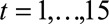
The baseline demographic characteristics by facility type and exposure categories as defined by cut-offs are shown in Tables 1 and 2. In both smelters and fabrication facilities, workers exposed above the median have lower frequencies of cardiovascular risk factors and other measures of overall health than workers exposed below, although the rates of IHD are similar or slightly higher among the exposed. The mean risk score decile among the smelter workers exposed above the median cut-off was 4.6 versus 5.0 for those exposed below the median. At the 10th percentile cut-off, these differences become more stark, with a mean risk score of 4.7 for those exposed above and 5.7 below. In the fabrication, workers had mean risk scores of 4.9 among those exposed above and 5.3 below for the median cut-off and 5.1 above and 5.2 below for the 10th percentile cut-off.

TABLE 1.

Smelter Worker Cohort Demographics, Time Varying Covariates, and Outcomes by PM2.5 Exposure Cut-off and Exposure Level at Baseline

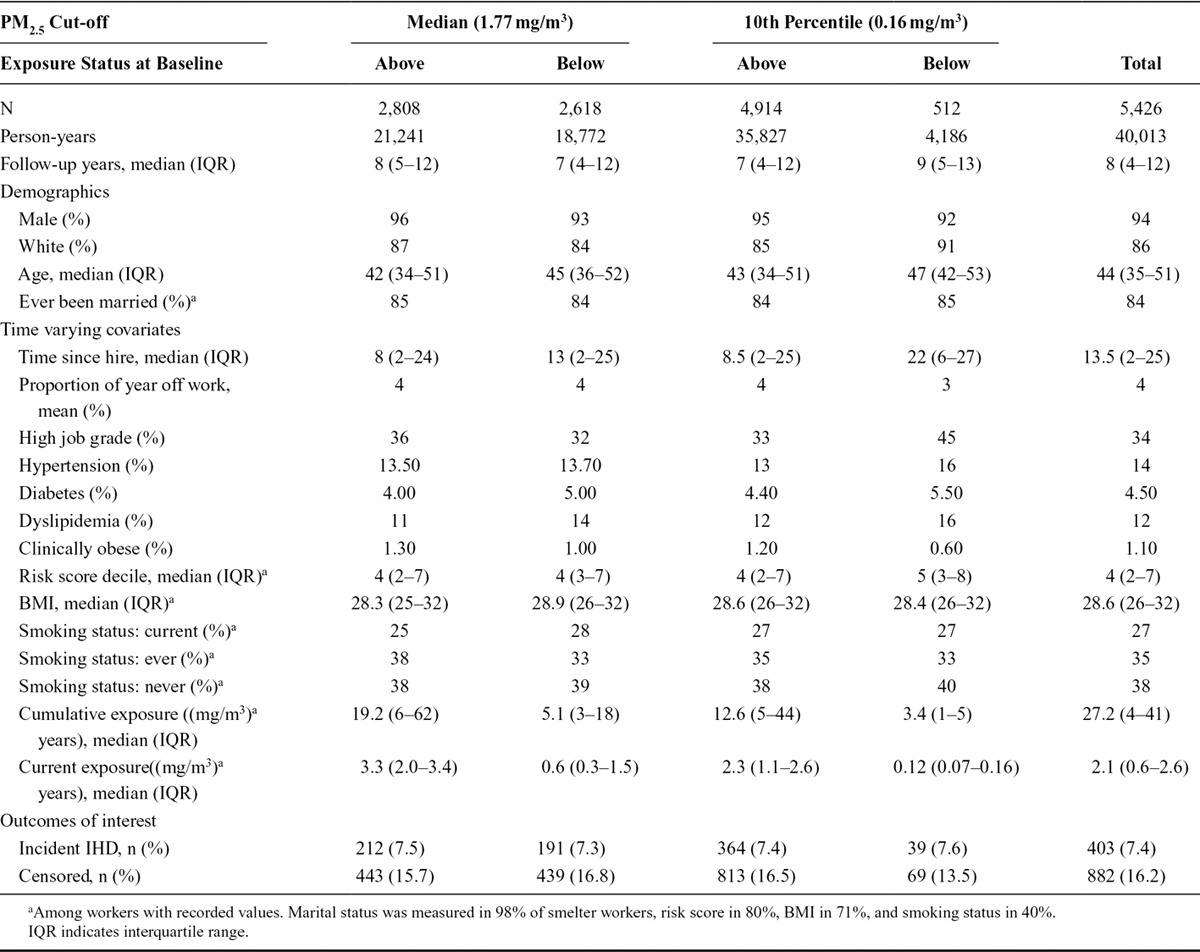
TABLE 2.

Fabrication Worker Cohort Demographics, Time Varying Covariates and Outcomes by PM2.5 Exposure Cut-off and Exposure Level at Baseline

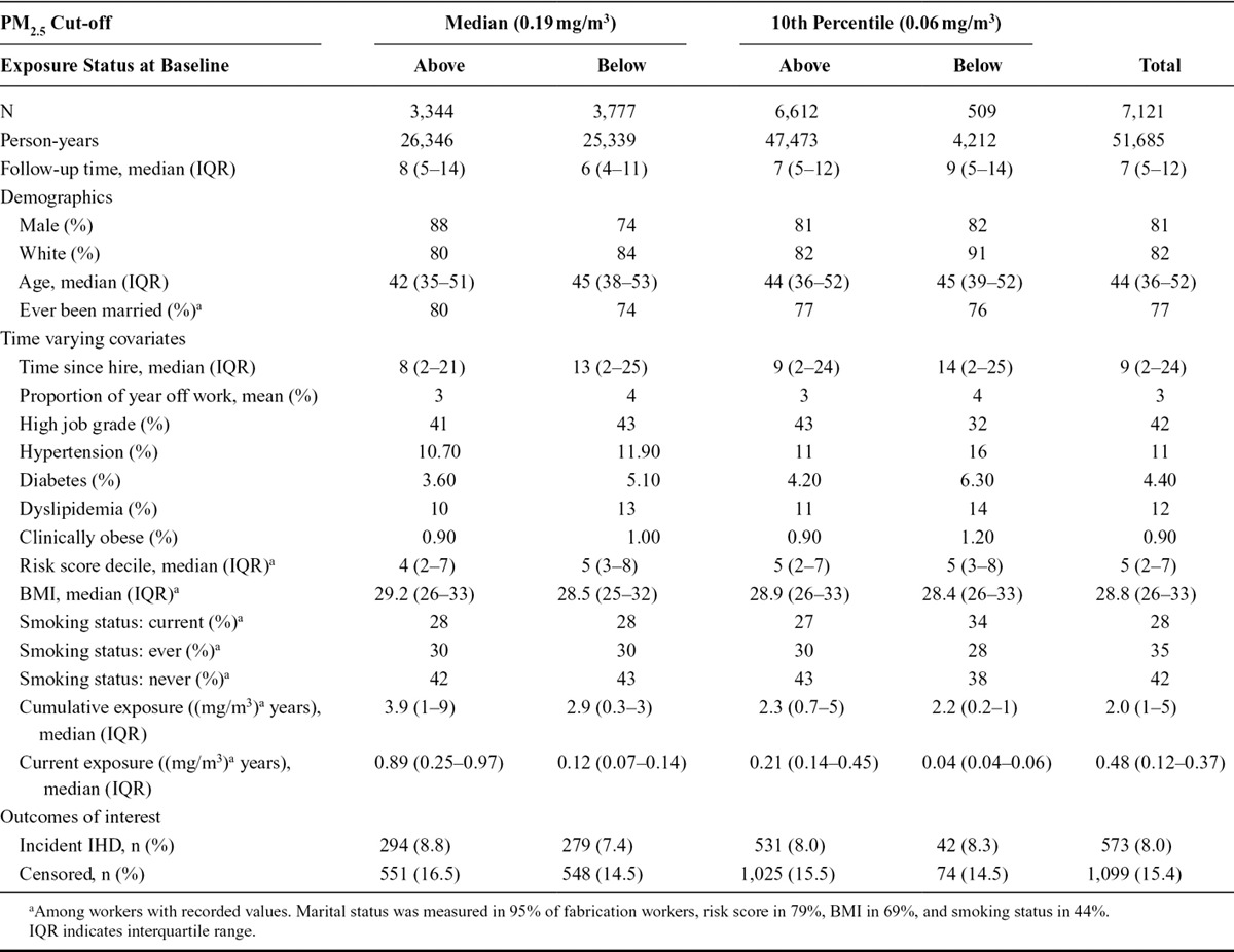
Table 3 presents the smelter and fabrication worker populations and incident disease counts by year of follow-up, with and without the restriction to those following the intervention regimen of staying in the same exposure category (for the median cut-off). This restriction resulted in the loss of 14% of the person-years and 12% of the incident cases from the fabrication analysis and in the loss of 17% of the person-years and 16% of the incident cases from the smelter analysis.

TABLE 3.

Worker Cohort Membership and Incident Ischemic Heart Disease Cases by Year of Follow-up and Facility Type for All Workers and Only Workers Exposed Consistently to Either Above or Below the Median (Fabricators: 0.19 mg/m3; Smelters: 1.77 mg/m3) Level of PM2.5

Figures 1, 2, 3 and 4 contain the marginal cumulative incidence curves estimated for each of the four exposure groups. Each curve estimates the percentage of the cohort that would remain undiagnosed with heart disease by the end of follow-up had all workers followed the intervention regimen.

FIGURE 1.

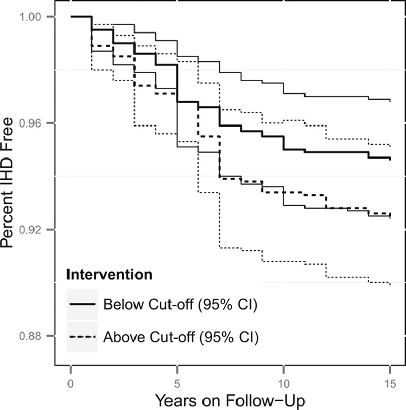
Estimated cumulative survival from IHD and 95% confidence intervals, adjusted for measured baseline and time-varying risk factors, among the smelter worker population if continuously exposed versus unexposed at the median cut-off of 1.77 mg/m³. The thick lines represent the point estimates, whereas the thinner lines represent the 95% confidence intervals, with the line types (dotted vs. solid) indicating if the estimate is for above or below the cut-off.

FIGURE 2.

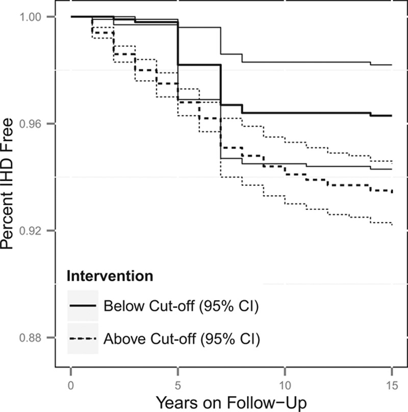
Estimated cumulative survival from IHD and 95% confidence intervals, adjusted for measured baseline and time-varying risk factors, among the smelter worker population if continuously exposed versus unexposed at the 10th percentile cut-off of 0.16 mg/m³. The thick lines represent the point estimates, whereas the thinner lines represent the 95% confidence intervals, with the line types (dotted vs. solid) indicating if the estimate is for above or below the cut-off.

FIGURE 3.

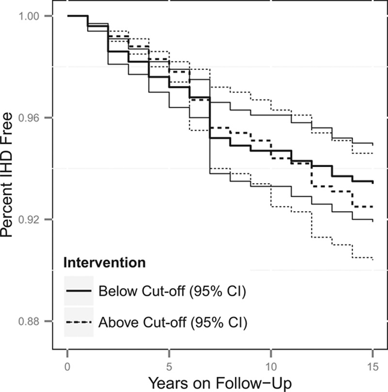
Estimated cumulative survival from IHD and 95% confidence intervals, adjusted for measured baseline and time-varying risk factors, among the fabricator worker population if continuously exposed versus unexposed at the median cut-off of 0.20 mg/m³. The thick lines represent the point estimates, whereas the thinner lines represent the 95% confidence intervals, with the line types (dotted vs. solid) indicating if the estimate is for above or below the cut-off.

FIGURE 4.

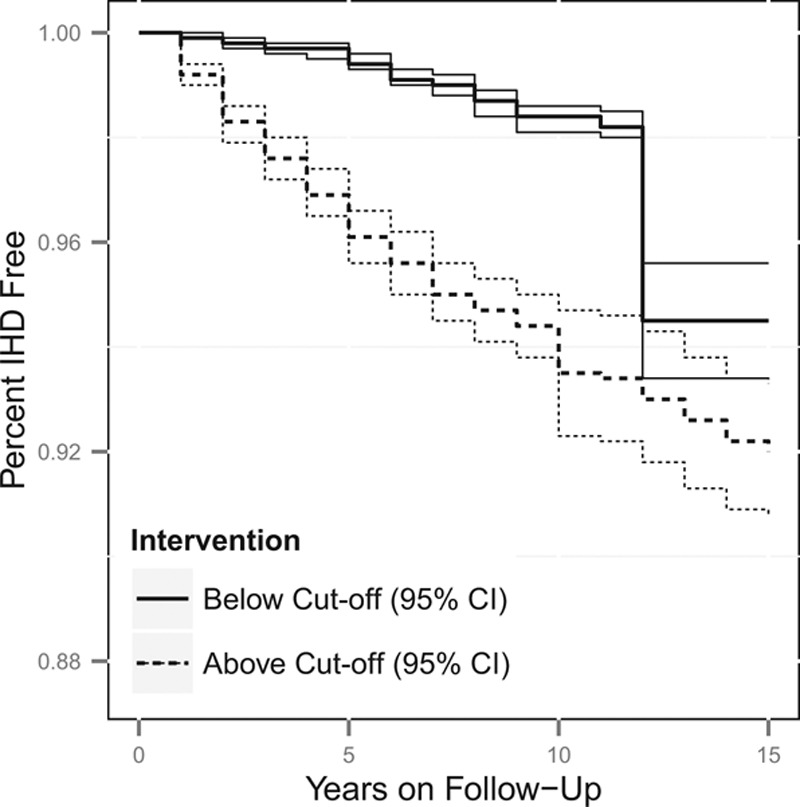
Estimated cumulative survival from IHD and 95% confidence intervals, adjusted for measured baseline and time-varying risk factors, among the fabricator worker population if continuously exposed versus unexposed at the 10th percentile cut-off of 0.06 mg/m³. The thick lines represent the point estimates, whereas the thinner lines represent the 95% confidence intervals, with the line types (dotted vs. solid) indicating if the estimate is for above or below the cut-off.

Table 4 contains the average treatment effects and rate ratios at year 15 for each of the four groups. The average treatment effect is the difference between the cumulative incidence of IHD predicted for a cohort always exposed above the cut-off and that for the same cohort always exposed below the cut-off. At year 15, the smelter worker sub-cohort, if constantly exposed above the median cut-off of 1.77 mg/m³ while remaining at work until 55 years, would experience a 2.1% (95% confidence interval = −1.3%, 5.5%) higher incidence of IHD compared with the same cohort if constantly exposed below the cut-off. For the 10th percentile cut-off of 0.16 mg/m³ in the smelter sub-cohort, the cumulative incidence of IHD would be higher by 2.9% (0.6%, 5.1%). Among the fabrication cohort, the estimated average treatment effect was 0.9% (−1.6%, 3.5%) for the median cut-off of 0.20 mg/m³ and 2.5% (0.8%, 4.1%) for the 10th percentile cut-off of 0.06 mg/m³. The unadjusted average treatment effect estimates in the smelter sub-cohort were 0.0% and 0.7% for the median and 10th percentile respectively, and 1.8% and 0.2% for the median and 10th percentile in the fabrication sub-cohort.

TABLE 4.

ATE and RR of Occupational Exposure to PM2.5 by Facility Type and Cut-off Level

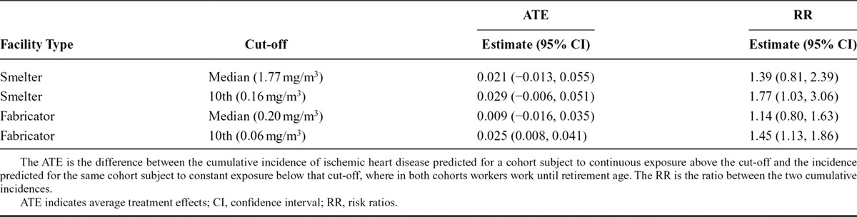
The estimation of marginal cumulative incidence also allows us to calculate causal risk ratios for the same exposure groups, by taking the ratio of the two incidences. Among the smelter sub-cohort, the average causal risk ratio (averaged over the 15 years of follow-up) was 1.4 (0.8, 2.4) at the median cut-off and 1.8 (1.0, 3.1) at the 10th percentile cut-off. Among the fabrication facility sub-cohort, the average causal risk ratio was 1.1 (0.8, 1.6) at the median cut-off and 1.5 (1.1, 1.9) at the 10th percentile cut-off.

DISCUSSION

These results provide evidence that increased risk of IHD is associated with cumulative occupational exposure to PM_2.5 in both the fabrication and smelter sub-cohorts. Prior analyses, using Cox models¹⁷ and inverse-probability weighted Cox marginal structural models,¹⁸ generated similar findings supporting a detrimental effect of exposure, although the effect measures differed. In contrast with the conventional analysis and similarly to results from the inverse-probability weighted Cox marginal structural model, we observed stronger associations in the smelters than in the fabrication. The TMLE estimate of the risk ratio returned smaller confidence intervals than those from the inverse-probability weighted estimate of the hazard ratio. In three of the four point estimates, we estimated larger effects using targeted minimum loss-based estimates than unadjusted estimates.

We applied longitudinal TMLE to adjust for the time-varying confounders on the causal pathway that characterize healthy worker survivor bias. The cohort demographics by exposure status (Tables 1 and 2) are consistent with the presence of this bias, and indicative of a pattern of behavior in which workers tend to be in lower-exposure jobs as cardiovascular risk, job tenure, and age increase. If a portion of the cardiovascular risk increase can be attributed to prior exposure, then the healthy worker survivor effect is operating and unbiased estimation of causal effects can only be accomplished using methods that can account for this.⁸ Pathway analysis¹⁸ was consistent with anecdotal evidence suggesting that the selection effects are stronger in the smelter environment where workers with high cardiovascular risk are ineligible for jobs with heat exposure.

We chose to use the TMLE procedure to generate estimates of our target exposure–response parameter. Estimators based on the this methodology have several attractive characteristics, relative to inverse probability weights or other g methods. The estimators are double-robust, in that they remain consistent if either the estimates of the outcome models (the series of iterated regressions) or the intervention models (gC or gA) are estimated consistently. These estimators are also efficient, in that if both the outcome models and the intervention models are consistently estimated they will have the lowest variance among all competitive estimators. For a full explanation of these properties and a comparison of TMLE with other causal approaches to estimation, see chapter 6 in van der Laan and Rose.¹⁵

A sensitivity analysis demonstrated that including workers who never had a high-confidence exposure estimate reduced the effect estimates.¹⁷ Corporate industrial hygienists collect measurements more frequently in areas where high exposures are expected. Thus, subjects with high exposures were preferentially selected into our cohort, although many lower exposure jobs were still measured with high confidence. If workers in low confidence jobs were substantially different from the rest of the population with respect to unmeasured factors prognostic of IHD then the restriction could result in selection bias. That said, we are certain that the restriction reduced exposure misclassification, whereas there is no reason to believe that the confidence measure is associated with these unmeasured factors.³² Therefore, we feel that our analysis restricted to workers in whom exposure was assessed with high-confidence generates a less biased effect estimate than analysis of the full cohort.

Censoring is defined in this analysis as leaving work when younger than 55 years. Leaving work is likely affected by health status caused by prior exposure, resulting in informative censoring that is not amenable to adjustment using standard methods. Furthermore, we are interested in the effects of exposure that do not act through leaving work. The choice of age 55 years represents a compromise between capturing the full effect of the exposure and reducing the reliance of the procedure on those unusual individuals who stay at work past eligibility for a full retirement. Sensitivity analysis demonstrated that the results were robust to the age cut-off; changing the age to 60 or 62 years did not substantially change the results.¹⁸ Continuing follow-up after work termination would give us the information needed to study the effects of PM_2.5 on post-retirement health.

We observed higher crude rates of IHD among the fabrication workers, and the marginal cumulative incidence estimates reflect this fact. As with any procedure, these estimates do not generalize to different populations with their own underlying risk and termination patterns. For example, heart disease rates among the fabrication workers, had they been exposed to the PM_2.5 in the smelters instead, cannot be inferred. Although the two sub-cohorts exhibit similar rates of chronic diseases, the risk scores were higher among the fabrication workers.

These results provide evidence that increased risk of IHD is associated with occupational exposure to PM_2.5 in both the fabrication and smelter sub-cohorts. We were able to adjust for possible time-varying confounders on the causal pathway through our use of the longitudinal TMLE procedure. We have not addressed the question of precisely when the biologically relevant exposure occurred (i.e., if IHD risk during time t is more dependent on exposure at time t or on exposures accumulated prior to time t). This question would be answered by estimating the indirect effect of cumulative exposure that does not travel through current exposure, a target parameter that deserves future research.

We observed excess IHD risk associated with PM_2.5 in both smelters and fabrication facilities where the composition and particle size distribution differ. In fabrication, the PM_2.5 is composed mostly of water-based metalworking fluids and in smelters, of inorganic materials, such as fluorides, alumina dust, metals, and related fumes.^5,22 Thus, our findings suggest that the total mass of PM_2.5 may be the common causal agent, although further study is needed to address this question. It is also possible that the observed relation between exposure to PM_2.5 and IHD could be due in part to coexposures in these workplaces, such as noise and heat.

The goal of causal inference is to make inference about counterfactual quantities, and unbiased estimation can proceed only if several assumptions are met. While we have a rich dataset that captures many of the salient aspects of health upon which workers might base their employment decisions, our dataset is administrative and unmeasured confounding remains a distinct possibility. We believe that we have limited positivity violations; there were no combinations of covariates that strongly predicted exposure status. The assumption of consistency, which is often subsumed by the use of nonparametric structural equation models,³⁴ may be more problematic. The dichotomization of exposure means that a range of different true exposure values and constituencies are contained in a single category. Future research with this cohort will involve investigating the shape of continuous exposure response curves through the use of TMLE to estimate of the parameters of marginal structural models.

A third of the workers in the cohort were currently employed before start of follow-up. Due to the fact that these prevalent workers did not leave work, we might expect them to be less susceptible to the exposures of interest than those who did leave. Our effect estimates are specific to the population we study; a cohort of all workers followed since hire might be reasonably expected to demonstrate a larger effect size.³⁵ In this study, follow-up was truncated at the termination of work, raising the possibility of collider bias due to informative censoring.³⁶ However, as with exposure, we believe we have measured key sources of this censoring. Our estimates are at risk for bias due to changes in follow-up time of the risk profile of newly hired workers, as those hired later could be followed up for fewer years due to administrative censoring.

For the sake of simplicity and computational efficiency, we chose to proceed with main-term logistic regression with limited variable selection. Both the efficiency and the unbiasedness of the targeted minimum loss-based estimator rely on consistently estimated models, so estimation could be improved with more flexible modelling procedures, such as cross-validated ensemble learners.³⁷ By implementing multiple imputation, we assumed missingness at random for the missing variables as well as a specific model form for the imputation model. Violations of this assumption or misspecification of the imputation model could result in bias. A sensitivity analysis showed that the results were robust to the removal of the smoking and BMI variables, indicating that they function as limited confounders in this dataset.

We applied TMLE in a longitudinal study to account for time-varying confounding and generated doubly-robust, efficient, substitution estimators of our parameters of interest. These parameters were used to create marginal incidence curves estimating the experience of the workforce if subjected to interventions on the exposure assignment and censoring mechanisms. Our analysis supports a causal connection between an accumulation of occupational exposure to PM_2.5 and the subsequent incidence of IHD.

Supplementary Material

ede-26-806-s001.doc ^{(1.1MB, doc)}

REFERENCES

- 1.Eisen EA, Robins JM, Picciotto S. Healthy worker effect in occupational studies. In: El-Shaarawi A, Piegorsch W, editors. Encyclopedia of Environmetrics. Chichister, UK: John Wiley & Sons; 2001. pp. 987–991. [Google Scholar]
- 2.Arrighi HM, Hertz-Picciotto I. The evolving concept of the healthy worker survivor effect. Epidemiology. 1994;5:189–196. doi: 10.1097/00001648-199403000-00009. [DOI] [PubMed] [Google Scholar]
- 3.Robins J. A new approach to causal inference in mortality studies with a sustained exposure period application to control of the healthy worker survivor effect. Math Model. 1986;7:1393–1512. [Google Scholar]
- 4.Greenland S, Judea P, James M. R. Causal diagrams for epidemiologic research. Epidemiology. 1999;10:37–48. [PubMed] [Google Scholar]
- 5.Robins JM, Hernán MA, Brumback B. Marginal structural models and causal inference in epidemiology. Epidemiology. 2000;11:550–560. doi: 10.1097/00001648-200009000-00011. [DOI] [PubMed] [Google Scholar]
- 6.Cole SR, Hernán MA, Robins JM, et al. Effect of highly active antiretroviral therapy on time to acquired immunodeficiency syndrome or death using marginal structural models. Am J Epidemiol. 2003;158:687–694. doi: 10.1093/aje/kwg206. [DOI] [PubMed] [Google Scholar]
- 7.Hernán MA, Brumback B, Robins JM. Marginal structural models to estimate the causal effect of zidovudine on the survival of HIV-positive men. Epidemiology. 2000;11:561–570. doi: 10.1097/00001648-200009000-00012. [DOI] [PubMed] [Google Scholar]
- 8.Cole SR, Richardson DB, Chu H, Naimi AI. Analysis of occupational asbestos exposure and lung cancer mortality using the g formula. Am J Epidemiol. 2013;177:989–996. doi: 10.1093/aje/kws343. [DOI] [PMC free article] [PubMed] [Google Scholar]
- 9.Dumas O, Le Moual N, Siroux V, et al. Work related asthma. A causal analysis controlling the healthy worker effect. Occup Environ Med. 2013;70:603–610. doi: 10.1136/oemed-2013-101362. [DOI] [PubMed] [Google Scholar]
- 10.Chevrier J, Picciotto S, Eisen EA. A comparison of standard methods with g-estimation of accelerated failure-time models to address the healthy-worker survivor effect: application in a cohort of autoworkers exposed to metalworking fluids. Epidemiology. 2012;23:212–219. doi: 10.1097/EDE.0b013e318245fc06. [DOI] [PubMed] [Google Scholar]
- 11.Neugebauer R, van der Laan M. Why prefer double robust estimators in causal inference?. J Stat Plan Inference. 2005;129:405–426. [Google Scholar]
- 12.van der Laan MJ, Gruber S. Targeted minimum loss based estimation of causal effects of multiple time point interventions. Int J Biostat. 2012;8 doi: 10.1515/1557-4679.1370. [DOI] [PubMed] [Google Scholar]
- 13.van der Laan MJ, Rose S. Targeted Learning. New York, NY: Springer; 2011. [Google Scholar]
- 14.van der Laan MJ, Rubin D. Targeted maximum likelihood learning. Int J Biostat. 2006;2:1–40. [Google Scholar]
- 15.Pope CA, III, Burnett RT, Thun MJ, et al. Lung cancer, cardiopulmonary mortality, and long-term exposure to fine particulate air pollution. JAMA. 2002;287:1132–1141. doi: 10.1001/jama.287.9.1132. [DOI] [PMC free article] [PubMed] [Google Scholar]
- 16.Chow JC, Watson JG, Mauderly JL. Health effects of fine particulate air pollution: lines that connect. J Air Waste Manag Assoc. 2006;56:1368–1380. doi: 10.1080/10473289.2006.10464545. [DOI] [PubMed] [Google Scholar]
- 17.Costello S, Brown DM, Noth EM, et al. Incident ischemic heart disease and recent occupational exposure to particulate matter in an aluminum cohort. J Expo Sci Environ Epidemiol. 2014;24:82–88. doi: 10.1038/jes.2013.47. [DOI] [PMC free article] [PubMed] [Google Scholar]
- 18.Neophytou AM, Costello S, Brown DM, et al. Marginal structural models in occupational epidemiology: application in a study of ischemic heart disease incidence and PM2.5 in the US aluminum industry. Am J Epidemiol. 2014;180:608–615. doi: 10.1093/aje/kwu175. [DOI] [PMC free article] [PubMed] [Google Scholar]
- 19.Fang SC, Cassidy A, Christiani DC. A systematic review of occupational exposure to particulate matter and cardiovascular disease. Int J Environ Res Public Health. 2010;7:1773–1806. doi: 10.3390/ijerph7041773. [DOI] [PMC free article] [PubMed] [Google Scholar]
- 20.Greenland S, Robins JM, Pearl J. Confounding and collapsibility in causal inference. Stat Sci. 1999;14:29–46. [Google Scholar]
- 21.Naimi AI, Cole SR, Westreich DJ, Richardson DB. A comparison of methods to estimate the hazard ratio under conditions of time-varying confounding and nonpositivity. Epidemiology. 2011;22:718–723. doi: 10.1097/EDE.0b013e31822549e8. [DOI] [PMC free article] [PubMed] [Google Scholar]
- 22.Noth EM, Dixon-Ernst C, Liu S, et al. Development of a job-exposure matrix for exposure to total and fine particulate matter in the aluminum industry. J Expo Sci Environ Epidemiol. 2014;24:89–99. doi: 10.1038/jes.2013.53. [DOI] [PMC free article] [PubMed] [Google Scholar]
- 23.Modrek S, Cullen MR. Health consequences of the “great recession” on the employed: evidence from an industrial cohort in aluminum manufacturing. Soc Sci Med. 2013;92:105–113. doi: 10.1016/j.socscimed.2013.04.027. [DOI] [PMC free article] [PubMed] [Google Scholar]
- 24.Kubo J, Goldstein BA, Cantley LF, et al. Contribution of health status and prevalent chronic disease to individual risk for workplace injury in the manufacturing environment. Occup Environ Med. 2014;71:159–166. doi: 10.1136/oemed-2013-101653. [DOI] [PMC free article] [PubMed] [Google Scholar]
- 25.van der Laan MJ, Petersen ML. Causal effect models for realistic individualized treatment and intention to treat rules. Int J Biostat. 2007;3:Article 3. doi: 10.2202/1557-4679.1022. [DOI] [PMC free article] [PubMed] [Google Scholar]
- 26.Bembom O, van der Laan MJ. A practical illustration of the importance of realistic individualized treatment rules in causal inference. Electron J Stat. 2007;1:574–596. doi: 10.1214/07-EJS105. [DOI] [PMC free article] [PubMed] [Google Scholar]
- 27.Bang H, Robins JM. Doubly robust estimation in missing data and causal inference models. Biometrics. 2005;61:962–973. doi: 10.1111/j.1541-0420.2005.00377.x. [DOI] [PubMed] [Google Scholar]
- 28.Peduzzi P, Concato J, Kemper E, Holford TR, Feinstein AR. A simulation study of the number of events per variable in logistic regression analysis. J Clin Epidemiol. 1996;49:1373–1379. doi: 10.1016/s0895-4356(96)00236-3. [DOI] [PubMed] [Google Scholar]
- 29.Schwab J, Lendle S, Petersen M, van der Laan M. ltmle: Longitudinal targeted maximum likelihood estimation. R package version 0.9.1. 2013. [Google Scholar]
- 30.Rubin D. Multiple Imputation for Nonresponse in Surveys. Chichister, UK: John Wiley; 1987. [Google Scholar]
- 31.Schafer JL. Analysis of Incomplete Multivariate Data. Boca Raton, FL: Chapman & Hall/CRC; 1997. [Google Scholar]
- 32.Blair A, Stewart P, Lubin JH, Forastiere F. Methodological issues regarding confounding and exposure misclassification in epidemiological studies of occupational exposures. Am J Ind Med. 2007;50:199–207. doi: 10.1002/ajim.20281. [DOI] [PubMed] [Google Scholar]
- 33.Rønneberg A. Mortality and cancer morbidity in workers from an aluminium smelter with prebaked carbon anodes–Part III: mortality from circulatory and respiratory diseases. Occup Environ Med. 1995;52:255–261. doi: 10.1136/oem.52.4.255. [DOI] [PMC free article] [PubMed] [Google Scholar]
- 34.Pearl J. Causal diagrams for empirical research. Biometrika. 1995;82:669–688. [Google Scholar]
- 35.Applebaum KM, Malloy EJ, Eisen EA. Left truncation, susceptibility, and bias in occupational cohort studies. Epidemiology. 2011;22:599–606. doi: 10.1097/EDE.0b013e31821d0879. [DOI] [PMC free article] [PubMed] [Google Scholar]
- 36.Picciotto S, Brown DM, Chevrier J, Eisen EA. Healthy worker survivor bias: implications of truncating follow-up at employment termination. Occup Environ Med. 2013;70:736–742. doi: 10.1136/oemed-2012-101332. [DOI] [PubMed] [Google Scholar]
- 37.van der Laan MJ, Polley EC, Hubbard AE. Super learner. Stat Appl Genet Mol Biol. 2007;6:Article 25. doi: 10.2202/1544-6115.1309. [DOI] [PubMed] [Google Scholar]
- 38.Greenland S, Robins JM. Identifiability, exchangeability, and epidemiological confounding. Int J Epidemiol. 1986;15:413–419. doi: 10.1093/ije/15.3.413. [DOI] [PubMed] [Google Scholar]
- 39.Hernán MA, VanderWeele TJ. Compound treatments and transportability of causal inference. Epidemiology. 2011;22:368–377. doi: 10.1097/EDE.0b013e3182109296. [DOI] [PMC free article] [PubMed] [Google Scholar]
- 40.Robins JM. Robust estimation in sequentially ignorable missing data and causal inference models. Proceedings of the American Statistical Association Section on Bayesian Statistical Science. 2000. pp. 6–10.