Significance
Quantitative knowledge of terrestrial carbon pathways and processes is fundamental for understanding the biosphere’s response to a changing climate. Carbon allocation, stocks, and residence times together define the dynamic state of the terrestrial carbon cycle. These quantities are difficult to measure and remain poorly quantified on a global scale. Here, we retrieve global 1° × 1° carbon state and process variables by combining a carbon balance model with satellite observations of biomass and leaf area (where and when available) and global soil carbon data. Our results reveal emergent continental-scale patterns and relationships between carbon states and processes. We find that conventional land cover types cannot capture continental-scale variations of retrieved carbon variables; this mismatch has strong implications for terrestrial carbon cycle predictions.
Keywords: carbon cycle, biomass, soil carbon, allocation, residence time
Abstract
The terrestrial carbon cycle is currently the least constrained component of the global carbon budget. Large uncertainties stem from a poor understanding of plant carbon allocation, stocks, residence times, and carbon use efficiency. Imposing observational constraints on the terrestrial carbon cycle and its processes is, therefore, necessary to better understand its current state and predict its future state. We combine a diagnostic ecosystem carbon model with satellite observations of leaf area and biomass (where and when available) and soil carbon data to retrieve the first global estimates, to our knowledge, of carbon cycle state and process variables at a 1° × 1° resolution; retrieved variables are independent from the plant functional type and steady-state paradigms. Our results reveal global emergent relationships in the spatial distribution of key carbon cycle states and processes. Live biomass and dead organic carbon residence times exhibit contrasting spatial features (r = 0.3). Allocation to structural carbon is highest in the wet tropics (85–88%) in contrast to higher latitudes (73–82%), where allocation shifts toward photosynthetic carbon. Carbon use efficiency is lowest (0.42–0.44) in the wet tropics. We find an emergent global correlation between retrievals of leaf mass per leaf area and leaf lifespan (r = 0.64–0.80) that matches independent trait studies. We show that conventional land cover types cannot adequately describe the spatial variability of key carbon states and processes (multiple correlation median = 0.41). This mismatch has strong implications for the prediction of terrestrial carbon dynamics, which are currently based on globally applied parameters linked to land cover or plant functional types.
The terrestrial carbon (C) cycle remains the least constrained component of the global C budget (1). In contrast to a relatively stable increase of the ocean CO2 sink from 0.9 to 2.7 Pg C y−1 over the past 40 y, terrestrial CO2 uptake has been found to vary between a net 4.1-Pg C y−1 sink to a 0.4-Pg C y−1 source, and accounts for a majority of the interannual variability in atmospheric CO2 growth. The complex response of terrestrial ecosystem CO2 exchanges to short- and long-term changes in temperature, water availability, nutrient availability, and rising atmospheric CO2 (2–6) remains highly uncertain in C cycle model projections (7). As a result, there are large gaps in our understanding of terrestrial C dynamics, including the magnitude and residence times of the major ecosystem C pools (8, 9) and rates of autotrophic respiration (10). Moreover, the impact of climatic extremes on C cycling, such as recent Amazon droughts (11), highlights the importance of understanding the terrestrial C cycle sensitivity to climate variability. To understand terrestrial CO2 exchanges in the past, present, and future, we need to better constrain current dynamics of ecosystem C cycling from regional to global scales.
C uptake, allocation, pool stocks, residence times, respiration, and disturbance together drive net CO2 exchanges (12) on subdaily to millennial timescales; these C state and process variables also determine the temporal sensitivity of the net C balance to climatic variability. For example, global changes in photosynthetic uptake could lead to a rapid response from short-lived C pools (such as foliage, fine roots, and litter) or a prolonged response from the long-lived C pools (such as woody biomass and soil C), with very different outcomes on ecosystem source–sink behavior. Quantitative knowledge of terrestrial C pathways is, therefore, central to understanding the temporal responses of the major terrestrial C fluxes—including heterotrophic respiration (13), fires (14, 15), and wetland CH4 emissions (16, 17)—to interannual variations in C uptake.
Although C dynamics have been extensively measured and analyzed at site level (18–21), the respiration and allocation of fixed C and its residence time within the major C pools are difficult and expensive to measure at site level and remain poorly quantified on global scales. As a result, global terrestrial C cycle models rely on land cover type-specific C cycling parameters—based on spatially preassigned plant functional types—to determine C fluxes and C pools (22). Globally spanning C cycle observations can provide a much-needed constraint on the spatial variability and associated dynamics of the terrestrial C cycle. Over the past decade, a growing number of datasets has enhanced understanding of the terrestrial C cycle, including global-scale canopy dynamics [National Aeronautics and Space Administration Moderate Resolution Imaging Spectroradiometer (MODIS) leaf area index (LAI)], empirically derived global soil C data [Harmonized World Soil Database (HWSD)] (23), satellite-based above- and belowground biomass (ABGB) maps for the tropics (24, 25), and Greenhouse Gases Observing Satellite CO2 and plant fluorescence (26, 27). These spatially and temporally explicit datasets provide an enhanced view of the terrestrial C cycle and can be used together to retrieve consistent global C state and process variables. Significant efforts in data-driven estimates of the global C fluxes have been made over the past decade. These efforts include estimates based on atmospheric CO2 concentrations (1, 28, 29), high-resolution global primary production maps (30) based on eddy covariance tower datasets (FLUXNET) (18), mean residence time of terrestrial C (31), ecosystem respiration dependence on temperature based on FLUXNET data (32), and global C cycle data assimilation systems (33).
Given an increasing number of C cycle observations, what remains an outstanding challenge is to produce a data-consistent analysis of terrestrial C cycling—including retrievals of C fluxes, C pools, autotrophic respiration, allocation fractions, and residence times—based on multiple global-scale earth observations and datasets. Current global-scale terrestrial biosphere models, because of their complexity and structures, are ill-equipped to ingest an ever-increasing volume of earth observations to estimate (rather than prescribe) model parameters based on the currently available observations. To overcome this challenge, we use a model–data fusion (MDF) approach to retrieve terrestrial C state and process variables during the period 2001–2010 without invoking plant functional type or steady-state assumptions. We bring together global MODIS LAI, a tropical biomass map (24), a soil C dataset (23), MODIS burned area (34), and a diagnostic ecosystem C balance model [Data Assimilation Linked Ecosystem Carbon Model version two (DALEC2)] (19, 35) to retrieve C state and process variables by producing a novel data-consistent and spatially explicit analysis of terrestrial C cycling on a global 1° × 1° grid (Fig. 1) [we henceforth refer to this MDF setup as the C data model framework (CARDAMOM)]. Specifically, we address the following questions: How is C uptake partitioned between the live biomass pools and respiration? What is the residence time of C within the major ecosystem C pools? How do estimates of C cycle states and processes vary spatially, and to what degree do emergent variable patterns match land cover maps? We use a Markov Chain Monte Carlo MDF algorithm to retrieve C state and process variables—and their associated uncertainty—within each 1° × 1° grid cell (Materials and Methods). The MDF approach retrieves the state and process variables that minimize the model mismatch against any available C cycle observations. Therefore, in the absence of extratropical biomass data or wintertime MODIS LAI observations, estimates of 2001–2010 C cycle state and process variables are achievable, albeit more uncertain.
Fig. 1.
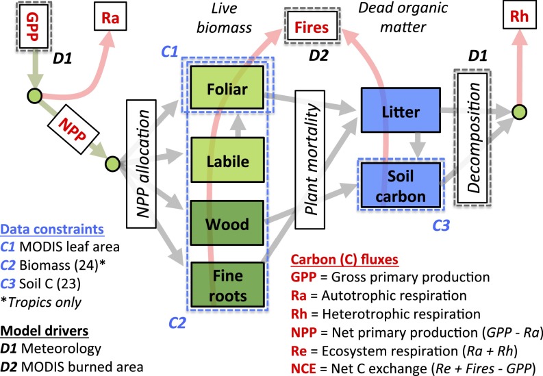
Diagnostic ecosystem C balance model DALEC2 (19, 35) and datasets used to retrieve 1° × 1° C state and process variables. GPP, a function of climate and foliar C, is partitioned into autotrophic respiration (Ra) and NPP. NPP is partitioned into the live biomass pools. Plant mortality provides input to the DOM pools. Heterotrophic respiration (Rh) is derived from decomposing DOM pools. Fire fluxes are derived from burned area data (35) and all C pools (SI Text, section S2). Within each 1° × 1° grid cell, we use a Bayesian MDF algorithm to retrieve C state/process variables and uncertainties; variables are retrieved without prior land cover type or steady-state assumptions. Data constraints consist of MODIS leaf area, total biomass (24) (tropics only), and soil C (23). Details on the Bayesian fusion approach are provided in Materials and Methods.
Results
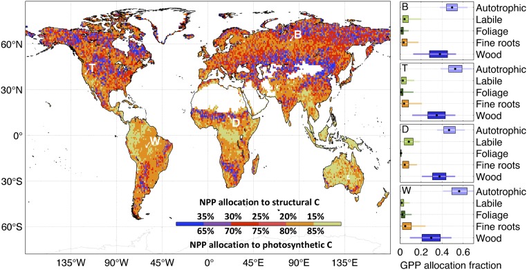
Distinct C allocation patterns emerge from our terrestrial C analysis (Fig. 2). Net primary production (NPP) allocation to structural biomass (wood and fine roots) is largely ≥80% (area-weighted 25th to 75th percentile range = 85–88%) in the wet tropics (<23° N/S; annual precipitation >1,500 mm) in contrast to the dry tropics (77–87%) and extratropical regions (73–82%). The highest NPP allocations to foliage (≥30%) spatially coincide with major grassland areas, including the North America prairies, the central Asia steppes, and the Sahel region in Africa. The dry tropics exhibit relatively high NPP allocation to labile C (7–14%) (Fig. S1), which reflects the increasing impact of seasonality on production as precipitation declines, requiring labile C stores for leaf flush. C use efficiency (CUE; equivalent to 1 − autotrophic respiration fraction) is overall lowest within the wet tropics (0.42–0.44) in contrast to dry tropical (0.45–0.50), temperate (23–55° N/S; 0.47–0.50), and high-latitude (>55° N/S; 0.49–0.50) areas.
Fig. 2.
Retrievals of NPP allocation to structural (wood and fine roots) and photosynthetic (labile and foliage) C pools. Allocation fractions were retrieved at 1° × 1° using a Bayesian MDF approach (Fig. 1). The GPP allocation fraction retrievals at locations B, T, D, and W are shown on the Right (black dot, median; box, 50% confidence range; line, 90% confidence range).
Fig. S1.
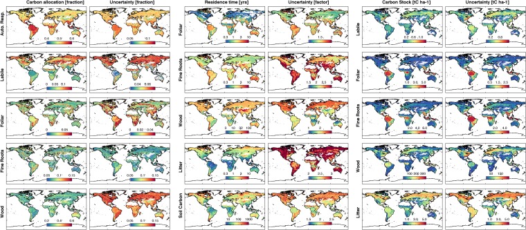
(Left) Posterior GPP C allocation to autotrophic respiration (equivalent to 1 − CUE), labile C, foliar C, fine roots, wood (mean; column 1), and associated uncertainty (SD; column 2). (Center) Posterior C residence time in foliar C; fine roots, wood, litter, and soil C (log-based mean; column 1); and associated uncertainty factors (based on logarithmic SD; column 2). (Right) Posterior mean 2001–2010 C stocks in labile, foliar, fine roots, wood, and litter C pools (mean; column 1) and associated uncertainties (SD; column 2).
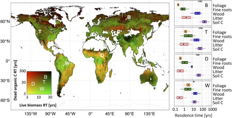
Live biomass and dead organic C residence times exhibit contrasting spatial features (r = 0.3) (Fig. 3). Within the majority of wet tropical land area (56%)—especially across most of the Amazon River (76%) and Congo River (69%) basins—the longest C residence time occurs within the woody pool (Fig. S1). In the dry tropics and extratropical latitudes, soil C residence times exceed wood C residence time by a median factor of 2.6 (1.6–4.3). Woody residence time is typically shorter in the dry tropics (8–19 y) compared with other biomes (wet tropics: 12–21 y; temperate latitudes: 21–29 y; and high latitudes: 25–28 y). Litter C residence time is typically longer in extratropical ecosystems (0.8–1.6 y) compared with tropical ecosystems (0.4–0.5 y). The longest foliar residence time (or leaf lifespan) occurs in the wet tropics and semiarid regions (Fig. S1).
Fig. 3.
Retrievals of C residence time (RT) in live biomass and dead organic C pools; residence times are retrieved at 1° × 1° using a Bayesian MDF approach (Fig. 1). Brown denotes ecosystems with high residence times for all C pools, green denotes ecosystems with long live biomass C residence times, and orange denotes ecosystems with low live biomass residence time. The residence times for individual C pools at locations B, T, D, and W are shown on the Right (black dot, median; box, 50% confidence range; line, 90% confidence range). Mean C residence times in ref. 31 are shown as gray boxes (50% confidence intervals) and black dots (medians).
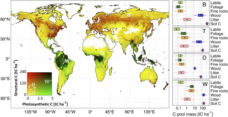
Overall, the wet tropics are characterized by relatively high structural C (>100 tC ha−1) and photosynthetic C (>2.5 tC ha−1) (Fig. 4): in contrast, the dry tropics and extratropical regions exhibit less structural and/or photosynthetic C. Foliar C stocks are typically larger in the wet tropics (2.8–4.7 tC ha−1) relative to other biomes (0.2–0.6 tC ha−1); similarly, fine root stocks are also greater in the wet tropics (4.0–5.3 tC ha−1) compared with other biomes (0.8–2.7 tC ha−1). Root:shoot (fine root C:leaf C) is lowest in the wet tropics (1.1–1.5) followed by the dry tropics (1.6–1.9) and extratropics (1.8–2.1). We find larger woody C uncertainties (1° × 1° 90% confidence range/median) in the extratropics (1.8–4.6) in contrast to tropical woody C (1.4–1.6) because of the latitudinal limits of the total ABGB map (24). Litter C is greater in high latitudes (2.4–3.4 tC ha−1) relative to temperate (0.6–2.4 tC ha−1) and tropical (0.2–2.6 tC ha−1) regions. High-latitude ecosystems have higher labile C stocks linked to seasonal leaf expansion (0.2–0.5 tC ha−1) relative to temperate (0.1–0.3 tC ha−1) and tropical (0.1–0.3 tC ha−1) ecosystems.
Fig. 4.
Retrieved mean photosynthetic (foliar and labile) and structural (wood and fine roots) C pool stocks; C stocks are retrieved at 1° × 1° using a Bayesian MDF approach (Fig. 1). Retrieved mean C stocks for each pool at locations B, T, D, and W are shown on the Right (black dot, median; box, 50% confidence range; line, 90% confidence range). Dark colors denote high-structural C/high-photosynthetic C ecosystems, green denotes low-structural C/high-photosynthetic C ecosystems, red denotes low-photosynthetic C/high-structural C ecosystems, and yellow denotes low-photosynthetic C/low-structural C ecosystems.
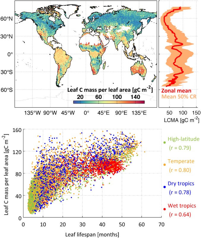
We find high leaf C mass per leaf area (LCMA) values in the wet tropics (85–97 gC m−2) and semiarid regions, such as the Sahel, southwestern United States, and the Australian continent (typically >100 gC m−2) (Fig. 5); LCMA estimates are lower (typically <80 gC m−2) in high latitudes and the dry tropics. We find a positive correlation between leaf lifespan and LCMA in high-latitude (r = 0.79), temperate (r = 0.80), dry tropical (r = 0.78), and wet tropical (r = 0.64) areas.
Fig. 5.
(Upper Left) Retrieved median 1° × 1° LCMA (in grams C per meter−2). (Upper Right) Zonal mean of median LCMA and 50% confidence range (CR). (Lower) LCMA against leaf lifespan for high latitudes (>55° N/S), temperate regions (23°–55° N/S), dry tropics (precipitation <1,500 mm; <23° N/S), and wet tropics (precipitation >1,500 mm; <23° N/S).
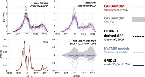
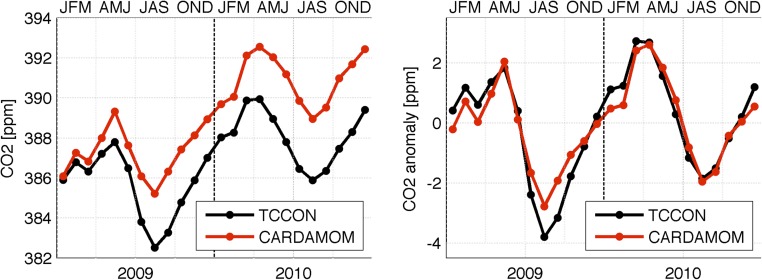
Global gross primary production (GPP; global 25th to 75th percentile = 91–134 Pg C y−1), ecosystem respiration (91–137 Pg C y−1), and fires (1.3–2.0 Pg C y−1) are broadly consistent with a terrestrial C model ensemble (22), data-driven estimates (36), and bottom-up inventories (37) (Fig. S2). The net C exchange uncertainty (−8 to +13 Pg C y−1) is an order of magnitude greater than mode net C exchange (NCE; −2 Pg C y−1); NCE latitudinal uncertainty is larger but comparable with the terrestrial C model ensemble range. Global atmospheric model CO2 concentrations based on CARDAMOM mode NCE fluxes are seasonally consistent [r2 = 0.93; root-mean-square error (RMSE) = 0.53 ppm CO2] with mean total column CO2 measurements (38) (Fig. S3). The mean integrated C residence time in ref. 31 is within the range of individual pool residence times at locations B, T, D, and W (Fig. 3). The 2001–2010 CARDAMOM analysis spatial and temporal LAI variability is consistent with the MODIS LAI constraints (r2 = 0.8; RMSE = 0.6 m2/m2). When alternative GPP (36), alternative model structure, or biased data constraints (±20%) are imposed at locations B, T, D, and W, 88% of median sensitivity analysis estimates are within ±50% of median C state and process variable retrievals (Fig. S4).
Fig. S2.
CARDAMOM zonal profiles of median GPP, ecosystem respiration, fires, and NCE (red). The 50% confidence range (C.R.) is depicted as a light gray-shaded area. The blue lines represent the eight global MsTMIP models (62) (details in SI Text, section S7). The dashed black line denotes the flux tower-derived GPP (36). The continuous black line denotes the Global Fire Emissions Database version 3 (GFEDv3) total C emissions (36).
Fig. S3.
The 2009–2010 GEOS-Chem model with CARDAMOM mode NCE compared against mean monthly total C column observing network (TCCON) atmospheric column measurements across 12 TCCON sites. Left shows atmospheric CO2 concentrations, and Right shows the linearly detrended CO2 anomalies. The detrended comparison Pearson’s r = 0.93, and RMSE = 0.53 ppm. JFM, AMJ, JAS, and OND denote consecutive 3-month periods between January and December.
Fig. S4.
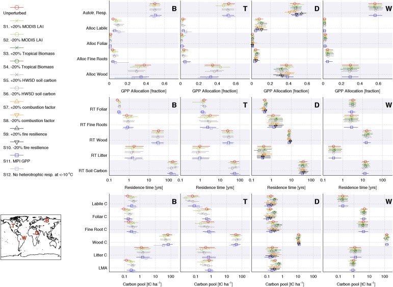
Posterior allocation fractions (alloc), residence times (RT), carbon pools (C), and leaf C mass per leaf area (LCMA) median and 50% confidence ranges shown for 1° × 1° grid cells B, T, D, and W for the unperturbed results (S0) and sensitivity experiments S1–S12. The coordinates of B, T, D, and W are reported in Materials and Methods (locations shown in Inset). Across all locations, 88% of median sensitivity analysis estimates (sensitivity tests S1–S12; SI Text, section S4) are within ±50% of unperturbed median C state and process variable retrievals.
Retrieved C cycle variables are broadly consistent with a range of in situ measurements (Table S1). Estimates of CUE within the Amazon River basin are comparable with the upper bound of recent measurements (0.32–0.47) (39). Recent estimates of extratropical forest C density (40) are, on average, 38% lower than CARDAMOM total biomass estimates within forested areas (although the forest biomass estimates are typically within the CARDAMOM 1° × 1° uncertainty). Estimates of mean Amazon woody C residence times (15–21 y) are lower but comparable with aboveground woody C residence times derived from site-level measurements (∼20–70 y) (20).
Table S1.
In situ observations and CARDAMOM posterior state and process variable estimates
| Measurement (region) | CARDAMOM range* | In situ observations (study) |
| Fine roots (Amazon River basin) | 9.2–10.8 tC ha−1 (2.8–11.5 tC ha−1) | 5–8 tC† ha−1‡ (64) |
| Fine roots (northeast United States; >30° N, >100° W) | 1.6–3.3 tC ha−1 (0.9–6.0 tC ha−1) | 1.25 tC† ha−1‡ (65) |
| Fine root residence time (northeast United States; >30° N, >100° W) | 1.1–1.5 y (0.9–3.2 y) | 0.83–1.25 y‡ (65) |
| Fine root residence time (global: where woody C is >10 tC ha−1) | 1.2–2.6 y (0.9–4.7 y) | 1.25–2.5 y§ (66) |
| Wood C residence time (Amazon River basin) | 15–21 y (9–24 y) | ∼20–70 y§ (20) (aboveground only) |
| CUE¶ (Amazon River basin) | 0.42–0.43 (0.42–0.45) | Amazon field sites: 0.32–0.47§ (39) |
| Fine root C (latitude >66° N) | 0.3–0.4 tC ha−1 (0.2–0.6 tC ha−1) | Arctic ecosystems: 0.1–5 tC ha−1§ (67) |
Area-weighted 25th to 75th percentile (5th to 95th percentiles) 1° × 1° C state and process variables (Materials and Methods).
Dry mass to C mass conversion factor = 0.5.
Individual site range.
Regional or global range.
CUE = 1 − autotrophic respiration fraction.
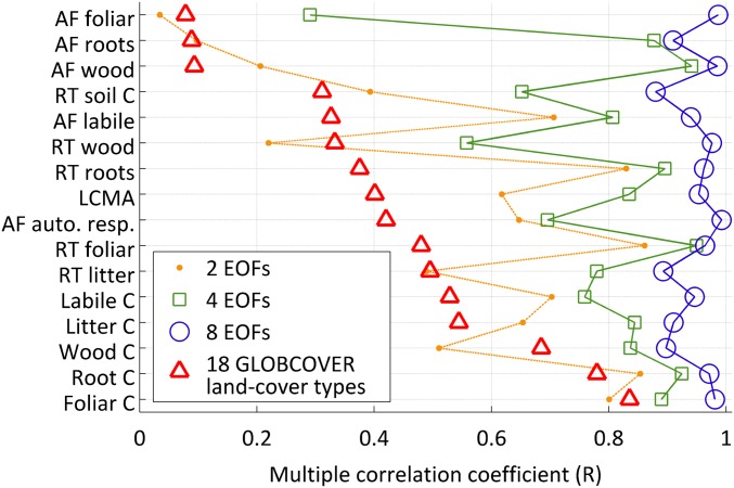
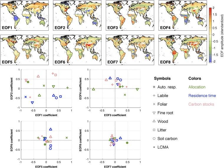
We find that 88–99% of C state and process variability is accounted for by eight empirical orthogonal basis functions (EOFs) (Fig. 6); in other words, retrieved C state and process variables are largely explained by eight modes of spatial variability (Fig. S5). On average, the Global Land Cover Map (GLOBCOVER) land cover classifications (41) (e.g., deciduous forests, evergreen forests, and grasslands) account for <50% of C state and process variability (median multiple correlation coefficient R = 0.41); GLOBCOVER land cover types best describe spatial variations in C stocks (0.5 ≤ R ≤ 0.8) followed by LCMA (R = 0.4), residence times (0.3 ≤ R ≤ 0.5), and allocation fractions (0.1 ≤ R ≤ 0.4).
Fig. 6.
Multiple correlation coefficients (R; x axis) of retrieved C state and process variables—allocation fractions (AF), residence times (RT), mean C pools, and LCMA (y axis)—against 18 GLOBCOVER land cover fractions and C variable primary EOFs. R denotes the ability of GLOBCOVER land cover types and primary EOFs to predict 1° × 1° state and process variables (R would equal one if all C state and process variables could be expressed as a linear sum of land cover fractions or EOFs).
Fig. S5.
Maps show eight primary 1° × 1° standardized EOFs 1–8 derived from a principal component analysis of standardized C state and process variables (SI Text, section S6). The two dominant modes (EOFs 1 and 2) together reflect first-order global variations in C state/process variables (cs) as a result of latitude and precipitation, whereas higher-order modes reflect increasingly complex spatial structures (we note, however, that EOFs 3–8 typically account for a smaller portion of cs spatial variability). Scatterplots show standardized EOFs 1–8 coefficients corresponding to each C state/process variable (shown as symbol–color combinations). The linear sum of standardized EOFs 1–4 (1–8) and the associated coefficients reproduce 29–95% (88–99%) of C state/process variability (Fig. 6).
Discussion
Typically, C allocation and residence time parameters are based on land cover types in global-scale terrestrial C cycle studies (refs. 9 and 22 among others); here, spatially broad allocation and residence patterns emerge instead as a result of the MDF approach. For example, high-biomass ecosystems throughout the wet tropics display similar C allocation, residence time, and LCMA configurations (Figs. 2–5). Similarly, we find that dead organic matter (DOM) C residence is generally longer in high latitudes (Fig. 3). Compared with conventional land cover types, EOFs 1–4 account for a larger degree of the spatial structures in retrieved C variables (Fig. 6); for most variables, the two dominant EOF modes—which together reflect first-order variations in latitude and global precipitation patterns (Fig. S5)—explain more spatial variability than GLOBCOVER land cover types. The mismatch between land cover types and retrieved variables has major implications for the estimation and prediction of terrestrial C cycling, which is currently based on small sets of globally applied parameters linked to land cover types. The importance of climate, biodiversity, fire, and anthropogenic disturbance in generating these mismatches needs to be explored in additional research (42).
It also is clear that plant traits vary across biomes (Figs. 2–4 and Fig. S1), not just at biome boundaries (43), and that there are continental-scale tradeoffs and correlations among traits (44). Our analysis is consistent with these viewpoints: for example, the emergent relationship between LCMA (proportional to leaf mass per area) and leaf lifespan (Fig. 5) matches the positive correlation found in global plant trait datasets (45). Evaluating global plant trait patterns emerging from CARDAMOM provides a novel opportunity for connections to theoretical and functional biodiversity research and a route to integrating this knowledge into predictive terrestrial C cycle modeling.
The residence times of major C stocks provide substantial insights into the sensitivity and potential future trajectories of the terrestrial C cycle. For example, land cover changes in the wet tropics may result in rapid DOM C losses given the relatively short DOM residence times (<30 y) (Fig. 3). In contrast, high-latitude C residence times are an order of magnitude higher (30–300 y), and therefore, shifts in C allocation or turnover rates are likely to result in long-lived C flux responses. Overall, given the predominant role of C residence times in future terrestrial uptake responses (9), the derived residence times provide a first-order estimate of ecosystem response times as a result of changes in C cycling regimes. However, we note that model structure is likely to be a major source of uncertainty in long-lived (>10 y) C flux predictions. For example, although reduced complexity models can capture some of the principal long-term (>10 y) DOM dynamics represented in earth system models (8), systematic errors in DOM dynamics can arise because of the underrepresentation of processes controlling DOM residence times (46, 47). We also note that our decadal analysis is unlikely to be able to capture slow feedback processes acting on longer timescales, such as permafrost remobilization and priming (48). The large allocation and stocks and short residence time of wood in the wet tropics indicate the potentially rapid postdisturbance regrowth and C accumulation (49). We note that fires are less frequent but major events within boreal ecosystems (50), and therefore, longer time periods are required for retrievals to fully account for the effect of fires on high-latitude C residence times.
C state and process variable retrievals are sensitive to the uncertainty characteristics of C cycle observations (35) and the prior parameter ranges (Table S2). We highlight that the current coverage and accuracy of C cycle observations (24, 51) remain major limiting factors in our approach. For example, extratropical C stock and residence time uncertainties are higher because of the absence of biomass observations. Undoubtedly, future estimates of globally spanning biomass density will provide a major constraint on CARDAMOM estimates of extratropical C state and process variables (52).
Table S2.
DALEC2 parameters, descriptions, and prior ranges (the DALEC2 equations are fully described in ref. 35)
| Parameters | Prior range |
| Allocation fractions | |
| Autotrophic respiration | 0.2–0.8* |
| Labile | 0.01–0.5 |
| Foliage | 0.01–0.5 |
| Fine roots | 0.01–0.5 |
| Wood | 0.01–0.5 |
| Turnover rates | |
| Woody C turnover rate | 2.5 × 10⁻⁵–10−3 d−1 |
| Fine root turnover rate | 10−4–10−2 d−1 |
| Litter turnover rate | 10−4–10−2 d−1 |
| Soil organic C turnover rate | 10−7–10−3 d−1 |
| Litter mineralization rate | 10−2–10−5 d−1 |
| Exponential temperature dependence | 0.018–0.08 |
| Canopy parameters | |
| Leaf onset day | 1–365.25 |
| Leaf fall day | 1–365.25 |
| Canopy efficiency | 5–50* |
| LCMA | 5–200 gC m−2 |
| Annual leaf loss fraction | 1/8–1 |
| Labile C release period | 10–100 d |
| Leaf fall period | 20–150 d |
| Initial C stocks (gC m−2) | |
| Labile C | 1–2,000 |
| Foliar C | 1–2,000 |
| Fine root C | 1–2,000 |
| Litter C | 1–2,000 |
| Above- and belowground wood | 1–100,000 |
| Soil C (1-m depth) | 1–200,000 |
Autotrophic respiration and canopy efficiency parameter log-normal prior distributions are described in SI Text, section S1.
Land to atmosphere C flux estimates could be used to further constrain CARDAMOM C fluxes (Fig. S2) and C cycle variables associated to nonsteady C states. For example, soil C residence time samples are negatively correlated with corresponding mean 2001–2010 NCE samples at locations B (r = −0.3), T (r = −0.4), D (r = −0.5), and W (r = −0.3); therefore, regional- or grid-scale estimates of NCE could provide a much-needed additional constraint on soil C residence time. CARDAMOM flux magnitude and uncertainty can be used as prior information in global atmospheric CO2 inversions; in turn, the assimilation of Greenhouse Gases Observing Satellite (26) and Orbiting Carbon Observatory 2 atmospheric CO2 observations (53) should further constrain CARDAMOM NCE estimates and their associated uncertainties. In this manner, nonsteady-state C fluxes can ultimately be reconciled with ecosystem state and process variables, such as C stocks and residence times.
The CARDAMOM approach provides a framework to test alternative model structures (54): in this manner, combined C cycle model parametric and structural uncertainties can be characterized, while ensuring consistency between models and global-scale datasets. This assessment would amount to a major step forward from conventional C cycle model intercomparison studies. Ultimately, an ensemble of models can be used to determine the degree to which retrievals of key C state and process variables are model-dependent. Moreover, alternative model structures could be used in CARDAMOM to assimilate globally spanning plant traits related to C cycling (55) and satellite observations, such as solar-induced fluorescence (27), vegetation optical depth (56), soil moisture (57, 58), and changes in aboveground biomass (25, 59, 60). We anticipate that the incorporation of additional datasets and alternative model structures into CARDAMOM will generate quantifiable reductions in retrieved C variable uncertainties and new ecological insights on the state of the terrestrial C cycle.
Materials and Methods
We grid MODIS LAI, ABGB (24), and HWSD topsoil and subsoil (0–100 cm) C density (23) at a 1° × 1° resolution (SI Text, section S1). DALEC2 is analytically described in ref. 35; an overview of DALEC2 C fluxes and pools is shown in Fig. 1. The 17 DALEC2 parameters (controlling the processes of photosynthesis, phenology, allocation, and turnover rates) and six initial C pools robustly characterize terrestrial ecosystem C balance (19). DALEC2 is a generic representation of C cycling, where plant functional types are not explicit; instead, model parameters are treated as unknown and independent quantities for each 1° × 1° grid cell (Table S2). We incorporate a fire C loss parameterization to account for seasonal and interannual variations in fire C fluxes from DALEC2 (SI Text, section S2). The model drivers consist of monthly time step European Centre for Medium-Range Weather Forecasts (ECMWF) Reanalysis Interim (ERA-interim) meteorology and MODIS burned area (34) at a 1° × 1° resolution.
For each 1° × 1° grid cell, we use Bayesian inference to retrieve the probability of DALEC2 model parameter xi (Table S2) given observational constraint Oi [henceforth p(xi|Oi)], where
| [1] |
In the expression, p(xi) is the prior parameter information, and p(Oi|xi) is the likelihood of xi with respect to Oi. We use a Markov Chain Monte Carlo algorithm to sample xi from p(xi|Oi); we henceforth refer to the retrieved DALEC2 parameter values at pixel i as yi. Within each grid cell, C allocation fractions, residence times within each C pool, stocks, LCMA, and associated C fluxes are derived from 4,000 samples of yi (SI Text, section S3). We, hence, obtain a probability density function for all C cycle variables within each 1° × 1° grid cell.
We do not impose plant functional type-specific prior parameter distributions or steady-state assumptions: p(xi) consists of ecologically viable parameter ranges (Table S2) and ecological and dynamical constraints (35). These constraints guarantee ecologically consistent parameter retrievals within a globally prescribed parameter space without imposing spatially explicit prior parameter information.
From the C state and process variable estimates within each 1° × 1° grid cell, we use 4,000 samples of yi to determine the mean, median, mode, and percentile ranges for each C state and process variable. In Figs. 2–4, we present C allocation, residence time, and C stock 5th, 25th, 50th, 75th, and 95th percentiles at four selected locations: B: 62.5°N, 81.5°E; T: 40.5°N, 120.5°W; D: 12.5°N, 20.5°E; and W: 7.5°S, 60.5°W. We chose B, T, D, and W as representative examples for C state and process variable values within each area (the full 1° × 1° C state and process variable maps are shown in Fig. S1). To determine the robustness of our C state and process variable estimates, we perform dedicated sensitivity tests to characterize the role of systematic errors in data constraints and model structure: we repeat our C variable retrievals using ±20% LAI, ±20% ABGB, ±20% HWSD, ±20% combustion coefficients, alternative GPP (36), and limited heterotrophic respiration at <0 °C (SI Text, section S4 and Table S3).
Table S3.
Sensitivity tests for C allocation, residence times, and C pool size estimates at locations B, T, D, and W
| Sensitivity test(s) | Description |
| S1 and S2 | +20% and −20% in LAI observations |
| S3 and S4 | +20% and −20% increases in biomass observations |
| S5 and S6 | +20% and −20% increases in HWSD soil C observations |
| S7 and S8 | +20%* and −20% increases in fire combustion factors |
| S9 and S10 | +20% and −20% increases in fire resilience factor |
| S11 | Use mean 1° × 1° aggregated MPI GPP (36) as driver |
| S12 | No heterotrophic respiration† under −10 °C |
Foliar combustion factor increase by 10% (from 0.9 to 0.99).
Respiration temperature dependence coefficient (19) set to zero at <−10 °C, scaled by unity at >0 °C, and scaled from zero to one between −10 °C and 0 °C.
We compare our results against in situ and regional observations of C allocation, pools, and residence times (SI Text, section S5), and we evaluate the resulting fluxes against atmospheric CO2 observations across 12 Total Carbon Column Observing Network sites (38) by incorporating NCE results in a 4D atmospheric transport model (29). To determine whether global land cover types can predict the spatial variability of our results, we conduct a multiple correlation coefficient analysis between C state and process variables and 18 GLOBCOVER land cover fractions at 1° × 1° (Figs. S5 and S6). We also used a principal component analysis on C state and process variables to retrieve the primary 1° × 1° EOFs. The details of the CARDAMOM results evaluation and analyses are fully described in SI Text, sections S5, S6, S7, and S8. The Pearson’s correlation coefficient is abbreviated as r throughout the text. All spatially derived r and RMSE values reported in the text are area-weighted. Retrieved C variable ranges—reported as area-weighted 25th to 75th percentile range—are derived from 1° × 1° mean allocation and C stocks, log-based mean C residence times (Fig. S1), and median LCMA values (Fig. 6). All CARDAMOM datasets presented in this study can be downloaded from datashare.is.ed.ac.uk/handle/10283/875.
Fig. S6.
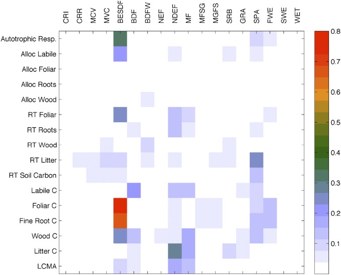
Pearson’s correlation coefficients (r2; shown in color bar) between GLOBCOVER land cover types fractions (x axis) and C state and process variables—allocation fractions (Alloc), residence times (RT), carbon pools (C), and leaf carbon mass per leaf area (LCMA) (y axis)—based on their correlation across all 1° × 1° grid cells within the global study area. BDF, closed broadleaved deciduous forest; BDFW, open broadleaved deciduous forest/woodland; BESDF, closed to open broadleaved evergreen or semideciduous forest; CRI, irrigated croplands; CRR, rain-fed croplands; FWE, closed to open broadleaved forest regularly flooded; GRA, closed to open herbaceous vegetation; MCV, mosaic cropland > vegetation; MF, closed to open mixed forest; MFSG, mosaic forest or shrub land > grassland; MGFS, mosaic grassland > forest or shrub land; MVC, mosaic vegetation > cropland; NDEF, open needle-leaved deciduous or evergreen forest; NEF, closed (>40%) needle-leaved evergreen forest; SPA, sparse vegetation; SRB, closed to open shrub land; SWE, forest or shrub land permanently flooded; WET, closed to open vegetation on flooded or waterlogged soil.
SI Text
S1. Global 1° × 1° Grid MDF.
Global datasets.
We grid the 30-s HWSD soil C density (based on national inventories of the top 1-m soil bulk density and organic C content) (23) and an ∼1 × 1-km above- and belowground pantropical biomass map (24) at 1° × 1°. We grid the MOD15A2 MODIS LAI product (1 × 1 km) and an MODIS burned area product (0.25° × 0.25°) (34) at a 1° × 1° monthly resolution for each month within the period 2001–2010. Although finer spatial/temporal resolutions can potentially be implemented, we chose a 1° × 1° monthly resolution as a consequence of the computational cost of our approach. We use European Centre for Medium-Range Weather Forecasts (ECMWF) Reanalysis Interim (ERA-interim) 1° × 1° monthly reanalysis products as DALEC2 drivers; ref. 35 has MODIS quality flag and ERA-interim driver details. We exclude 1° × 1° grid cells where desert and ice-covered areas account for more than 90% of the grid cell land cover (based on GLOBCOVER 2009 global land cover maps) (41), because their role in the terrestrial C cycle is negligible.
MDF.
Within each 1° × 1° grid cell i, we use the 1° × 1° aggregated biomass (tropics only), soil C, and MODIS LAI datasets (observations Oi) to constrain DALEC2 parameter xi (for a complete description of the DALEC2 model and C pools, we refer the reader to ref. 35 and references therein). We implement a Metropolis–Hastings Markov Chain Monte Carlo (MHMCMC) (33, 35) to determine the probability of xi given observational constraints Oi (expression 1).
The prior ranges of DALEC2 parameter xi are shown in Table S2. We also imposed a prior log-normal distribution on autotrophic respiration fraction xi,a (autotrophic respiration = 0.5 × 1.2±1) and a prior log-normal distribution on canopy efficiency xi,c (canopy efficiency parameter = 17.5 × 1.2±1), where ±1 represents a normal distribution with mean = 0 and variance = 1. These constraints yield a range of results that is broadly consistent with the global GPP range reported in ref. 30 and represent the range of autotrophic respiration estimates reported in ref. 61. The prior parameter probability p(xi) is, therefore, expressed as
| [S1] |
where pBW(xi) is the prior parameter probability described in ref. 35. Within each 1° × 1° grid cell, we prescribe an uncertainty factor of 1.5 to mean 2001–2010 HWSD soil C and total ABGB density (i.e., mean labile + foliar + fine roots + wood) and an uncertainty factor of 2 to mean monthly MODIS LAI observations. For total biomass, given that the maximum entropy algorithm used in ref. 24 was based on bins of 12.5 tC ha−1, we anticipate that low-biomass density values (such as the edges of the Sahel and Kalahari Deserts) exhibit comparable uncertainty. We, therefore, prescribe an uncertainty factor of max(1.5, 12.5/Bi), where Bi is the total biomass density, and the max function denotes the maximum of the two values. The likelihood function p(Oi|xi) is, therefore, expressed as
| [S2] |
where Oij and Uij are the jth observations and uncertainty factors at location i, and Mij is the equivalent DALEC2 model output based on parameter vector xi [we note that Oij, Uij, and Mij are log-transformed; e.g., for a soil C value of 100 tC ha−1, Oij = log(100) and Uij = log(1.5)]. For each LAI observation, Mij is the DALEC2 foliar C (on the corresponding month) divided by LCMA. For biomass and soil C, Mij is the DALEC2 soil C stock and mean live biomass (labile + foliar + fine roots + wood) on January 1, 2001. For the analytical description of DALEC2, the MHMCMC algorithm, and pBW(xi), we refer the reader ref. 35 and references therein; the DALEC2 fire module is described in SI Text, section S3.
Ecological and dynamical constraints.
The 12 ecological and dynamical constraints (EDCs; EDCs 1–12) (35) are a component of the prior parameter probability pBW(xi), and consist of relative constraints on allocation parameters, turnover rates, growth rates, exponential decays, and steady-state proximity. When steady state is not assumed, steady-state proximity conditions are necessary to distinguish between real and nonsensical C pool trajectories (35). We developed a simpler numeric equivalent of the steady-state proximity EDCs (EDCs 9–12) to account for the stochastic C losses from fires. For each pool, we derive the steady-state proximity factor () as follows:
| [S3] |
where and are the mean inputs and outputs, respectively, from each pool. We impose a steady-state proximity condition of 0.5 > > 2 for each pool.
We found that EDC 8—the EDC limiting rapid exponential pool trajectories—was excessively rigid for relatively small amounts of exponential pool trajectories (which can occur naturally and/or as a model artifact). Here, we use a simpler approach to minimize the rapid exponential decay of C pools: we ensure that the steady-state proximity of each C pool at time 0 − Sprox(jan2001) is within 0.05 of Sprox; i.e.,
| [S4] |
can be derived as
| [S5] |
where is the mean January C pool stock and C(jan2001) is the C pool stock in January of 2001. The CARDAMOM code used in this manuscript (DALEC2 model, EDCs, and adaptive MHMCMC) is available on request.
S2. DALEC2 Fire Module.
To determine the monthly C losses from fires at time t, we determine the monthly fraction of each grid cell burned, Barea(t), based on the MODIS-derived burned area product (34). At each monthly time step, the fire losses within each 1° × 1° grid cell are derived as
| [S6] |
where Fe(t) is the total fire C emissions at time t, kfactor(p) is the combustion factor for pool p, and C(p,t) is the C in pool p at time t. We also impose a resilience factor r to the remaining pools within the burned area: for the live biomass pools, a fire–mortality flux is derived from the uncombusted C pools as
| [S7] |
The fire–mortality C flux from foliage, roots, and labile is deposited into the litter pool, and fire–mortality C flux from wood is transferred to the soil C pool. Equally, 1 − r of uncombusted litter C is transferred to the soil C pool. The kfactor values for labile (0.1), foliar (0.9), root (0.1), wood (0.1), litter (0.5), and soil C (0.01) are broadly equivalent to the kfactor values used by the Global Fire Emission Database (37). We apply a resilience factor of r = 0.5. The sensitivity calculations associated with kfactor(p) and rf are described in SI Text, section S4.
S3. Global State and Process Variables.
The spatial distributions of individual C pool allocation fractions, residence times, and stocks are shown in Fig. S1. The residence time for each C pool at grid cell i is derived as
| [S8] |
where is the mean pool size, is the mean daily C pool input, and is the mean daily change in pool size throughout 2001–2010 for the jth parameter vector sample of yi [i.e., , , and are calculated from DALEC2 output driven with jth parameter vector sample of yi]. Mean live biomass (DOM) pool residence times are derived based on Eq. S8, where , , and are the total live biomass (DOM) C corresponding to jth parameter vector sample of yi. Leaf lifespan is equivalent to RTfoliar. Reported global and zonal 25th to 75th percentile ranges of total annual fluxes were derived from the sum of monthly 1° × 1° 25th and 75th percentiles for each flux multiplied by the 1° × 1° grid cell area; the same approach was used to derive median fluxes and mode NCE. Monthly mode NCE within each 1° × 1° grid cell was derived by binning NCE samples into 0.01 gC m−2 d−1 intervals.
S4. Sensitivity Tests.
We determine the sensitivity of C allocation, residence times, and C pool size estimates at locations B, T, D, and W (the B, T, D, and W coordinates are reported in the Materials and Methods) to LAI, biomass, and soil C data constraints (sensitivity tests S1–S6); fire combustion and resilience factor coefficients (sensitivity tests S7–S10); the use of Max Planck Institute GPP product (MPI GPP) (36) instead of the default DALEC GPP (19) (sensitivity test S11); and the suppression of heterotrophic respiration under −10 °C (sensitivity test S12). The sensitivity experiments are summarized in Table S3. The results of the sensitivity tests are shown in Fig. S4.
S5. Comparison Against in Situ and Regional Observations.
CARDAMOM results are compared against a range of in situ measurements in Table S1. We compare each in situ measurement against the 50% and 90% confidence ranges of the mean 1° × 1° values within the stated region. Comparison details and footnotes are included in Table S1. We also compare CARDAMOM total biomass against the extratropical Envisat Advanced Synthetic Aperture Radar forest biomass map (BIOMASAR map) (40) aggregated to 1° × 1°. The CARDAMOM to BIOMASAR comparison is conducted for the total biomass across all 1° × 1° areas with at least 95% BIOMASAR map coverage; total BIOMASAR biomass within those areas is 38% lower than CARDAMOM biomass. We note that lower than expected LCMA estimates in boreal ecosystems (Fig. 6) could be explained by (i) understory plant traits (linked to deciduous shrubs) or (ii) seasonal MODIS LAI biases (52). In particular, the significant correlation between LCMA and leaf lifespan suggests that retrieved LCMA accuracy could be strongly linked to seasonal biases in MODIS LAI.
S6. Comparison with GLOBCOVER Land Cover Types and EOFs.
For each 1° × 1° grid cell I, we determine the fraction of each GLOBCOVER (41) land cover type L: FL(i). We then determine the Pearson’s correlation coefficients (rLS values) between fL (the vector of all 1° × 1° land cover type L fractions) and each C state and process variable vector cS (the vector of each 1° × 1° state and process variable): state or process variables (denoted by subscript S) consist of allocation fractions, C residence times, C pool sizes, and LCMA. The rLS2 values between each GLOBCOVER land cover type fraction L and each C state/process variable S are shown in Fig. S6. The land cover categories are irrigated croplands, rain-fed croplands, mosaic cropland > vegetation, mosaic vegetation > cropland, closed to open broadleaved evergreen or semideciduous forest, closed broadleaved deciduous forest, open broadleaved deciduous forest/woodland, closed (>40%) needle-leaved evergreen forest, open needle-leaved deciduous or evergreen forest, closed to open mixed forest, mosaic forest or shrub land > grassland, mosaic grassland > forest or shrub land, closed to open shrub land, closed to open herbaceous vegetation, sparse vegetation, closed to open broadleaved forest regularly flooded, forest or shrub land permanently flooded, and closed to open vegetation on flooded or waterlogged soil (53).
The multiple correlation coefficient RS between C state/process variable S and 18 GLOBCOVER land cover type fractions is derived as
| [S9] |
where rS is the 1 × 18 vector of correlations coefficients between state/process variable vector cS and 18 1° × 1° land cover type fraction vectors fL, rsT is the transpose of rs, and is the inverse of the correlation matrix RLL, which contains the intercorrelations between 18 land cover type fraction vectors fL. RS is equivalent to the maximum correlation (Pearson’s r2) between the spatial variability of C state/process variable cS and the best-fitting linear combination of land cover type fraction fL. The resulting RS values are shown in Fig. 6.
We also use a multiple correlation coefficient analysis on the empirical orthogonal functions (EOFs; “primary modes” of variability) of all cs. We conducted a principal component analysis to derive the eight primary EOFs [EOFs were derived using the pca.m function in Matlab; each cs vector is centered at zero and scaled to the standard deviation (SD) of cs]. Standardized EOFs (normalized by EOF SD) and EOF coefficients are shown in Fig. S5. The EOF maps exhibit the primary modes of cs variability in space; for each cs, the maximum spatial variability explained by EOFs 1−N is the sum of standardized EOFs 1−N multiplied by their associated coefficients. EOF multiple correlation coefficients—RS(EOF)—were derived for the primary two, four, and eight EOFs based on Eq. S9, where RLL is the identity matrix (given that EOFs are orthogonal). RS(EOF) results are shown in Fig. 6.
S7. Comparison Against the Multiscale Synthesis and Terrestrial Model Intercomparison Project.
We compare GPP, ecosystem respiration, and NCE against the Multiscale Synthesis and Terrestrial Model Intercomparison Project (MsTMIP) terrestrial biosphere model ensemble version 1.0 (62) NCE (note that total C exchange is reported as net ecosystem exchange by MsTMIP). The 0.5° × 0.5° monthly GPP, total (heterotrophic and autotrophic) respiration, and NCE values for 2001–2010 based on the BG1 simulation were downloaded from nacp.ornl.gov/mstmipdata/ and aggregated to a 1° × 1° grid [the BG1 simulation includes time-varying nitrogen deposition, atmospheric CO2, and land use history (22)]. The eight MsTMIP models are shown in Fig. S2: for the sake of brevity, we did not label individual models.
S8. Atmospheric CO2 Comparison.
We incorporated the 2009–2010 CARDAMOM monthly mode NCE values into the Goddard Earth Observing System 4D chemistry and transport model (GEOS-Chem) (29). The GEOS-Chem model simulations are based on GEOS-Chem version 8.2 driven by the National Aeronautics and Space Administration GEOS-5 meteorological fields. In addition to NCE, fossil fuel emissions and oceanic surface CO2 fluxes are prescribed (55). We compared the 2009–2010 GEOS-Chem model CO2 concentrations against the monthly mean anomaly across 12 total C column observing network sites (38): Bialystok, Poland; Darwin, Australia; Eureka, Canada; Garmisch, Germany; Karlsruhe, Germany; Lauder, New Zealand; Lauder, New Zealand; Lamont, Oklahoma; Orleans, France; Park Falls, Wisconsin; Sodankyla, Finland; and Wollongong, Australia. Details of the GEOS-Chem total C column observing network comparison are reported in ref. 63 and references therein. We note that the uncertainty in the GEOS-Chem trend stemming from the CARDAMOM flux uncertainty is substantial: global NCE 25th to 75th percentile = −8 − +13 Pg C y−1, which roughly corresponds to a ±5-ppm growth rate (1). To evaluate the CARDAMOM seasonal NCE variability, we compare the linearly detrended model and observations (Fig. S3).
Acknowledgments
A.A.B., J.-F.E., L.F., and M.W. were funded by the NERC National Centre for Earth Observation. I.R.v.d.V. was financially supported under The Netherlands Organization for Scientific Research Project VIDI: 864.08.012. This work made use of the Edinburgh Compute and Data Facility resources. The research leading to these results received funding from European Union’s FP7 (2007–2013) Grant 283080 (Project GEOCARBON). The Total Carbon Column Observing Network (TCCON) is supported by the National Aeronautics and Space Administration (NASA) Carbon Cycle Science Program through a grant to the California Institute of Technology. Part of this research was carried out at the Jet Propulsion Laboratory, California Institute of Technology under a contract with NASA.
Footnotes
The authors declare no conflict of interest.
This article is a PNAS Direct Submission.
Data deposition: The outputs reported in this paper have been deposited in an online digital repository of multidisciplinary research datasets produced at the University of Edinburgh, datashare.is.ed.ac.uk/handle/10283/875.
This article contains supporting information online at www.pnas.org/lookup/suppl/doi:10.1073/pnas.1515160113/-/DCSupplemental.
References
- 1.Le Quéré C, et al. The global carbon budget 1959–2011. Earth Syst Sci Data. 2013;5(1):165–185. [Google Scholar]
- 2.Gatti LV, et al. Drought sensitivity of Amazonian carbon balance revealed by atmospheric measurements. Nature. 2014;506(7486):76–80. doi: 10.1038/nature12957. [DOI] [PubMed] [Google Scholar]
- 3.Dieleman WIJ, et al. Simple additive effects are rare: A quantitative review of plant biomass and soil process responses to combined manipulations of CO2 and temperature. Glob Chang Biol. 2012;18(9):2681–2693. doi: 10.1111/j.1365-2486.2012.02745.x. [DOI] [PubMed] [Google Scholar]
- 4.Keenan TF, et al. Increase in forest water-use efficiency as atmospheric carbon dioxide concentrations rise. Nature. 2013;499(7458):324–327. doi: 10.1038/nature12291. [DOI] [PubMed] [Google Scholar]
- 5.Reich PB, Hobbie SE. Decade-long soil nitrogen constraint on the CO2 fertilization of plant biomass. Nat Clim Chang. 2013;3(3):278–282. [Google Scholar]
- 6.Schimel D, Stephens BB, Fisher JB. Effect of increasing CO2 on the terrestrial carbon cycle. Proc Natl Acad Sci USA. 2015;112(2):436–441. doi: 10.1073/pnas.1407302112. [DOI] [PMC free article] [PubMed] [Google Scholar]
- 7.Cox PM, et al. Sensitivity of tropical carbon to climate change constrained by carbon dioxide variability. Nature. 2013;494(7437):341–344. doi: 10.1038/nature11882. [DOI] [PubMed] [Google Scholar]
- 8.Todd-Brown KEO, et al. Causes of variation in soil carbon simulations from CMIP5 Earth system models and comparison with observations. Biogeosciences. 2013;10(3):1717–1736. [Google Scholar]
- 9.Friend AD, et al. Carbon residence time dominates uncertainty in terrestrial vegetation responses to future climate and atmospheric CO2. Proc Natl Acad Sci USA. 2014;111(9):3280–3285. doi: 10.1073/pnas.1222477110. [DOI] [PMC free article] [PubMed] [Google Scholar]
- 10.Atkin OK, et al. Global variability in leaf respiration in relation to climate, plant functional types and leaf traits. New Phytol. 2015;206(2):614–636. doi: 10.1111/nph.13253. [DOI] [PubMed] [Google Scholar]
- 11.Lewis SL, Brando PM, Phillips OL, van der Heijden GMF, Nepstad D. The 2010 Amazon drought. Science. 2011;331(6017):554. doi: 10.1126/science.1200807. [DOI] [PubMed] [Google Scholar]
- 12.Luo Y, Weng E. Dynamic disequilibrium of the terrestrial carbon cycle under global change. Trends Ecol Evol. 2011;26(2):96–104. doi: 10.1016/j.tree.2010.11.003. [DOI] [PubMed] [Google Scholar]
- 13.Trumbore S. Carbon respired by terrestrial ecosystems - recent progress and challenges. Glob Chang Biol. 2006;12(2):141–153. [Google Scholar]
- 14.Randerson JT, et al. Fire emissions from C3 and C4 vegetation and their influence on interannual variability of atmospheric CO2 and δ13CO2. Global Biogeochem Cycles. 2005;19(2):GB2019. doi: 10.1002/2014GB004890. [DOI] [PMC free article] [PubMed] [Google Scholar]
- 15.Bloom AA, et al. Remote‐sensing constraints on South America fire traits by Bayesian fusion of atmospheric and surface data. Geophys Res Lett. 2015;42(4):1268–1274. [Google Scholar]
- 16.Bloom AA, Palmer PI, Fraser A, Reay DS. Seasonal variability of tropical wetland CH4 emissions: The role of the methanogen-available carbon pool. Biogeosciences. 2012;9(8):2821–2830. [Google Scholar]
- 17.Melton JR, et al. Present state of global wetland extent and wetland methane modelling: Conclusions from a model intercomparison project (WETCHIMP) Biogeosciences. 2013;10(2):753–788. [Google Scholar]
- 18.Baldocchi D, et al. FLUXNET: A new tool to study the temporal and spatial variability of ecosystem-scale carbon dioxide, water vapor, and energy flux densities. Bull Am Meteorol Soc. 2001;82(11):2415–2434. [Google Scholar]
- 19.Williams M, Schwarz PA, Law BE, Irvine J, Kurpius MR. An improved analysis of forest carbon dynamics using data assimilation. Glob Chang Biol. 2005;11(1):89–105. [Google Scholar]
- 20.Malhi Y, Saatchi S, Girardin C, Aragao LEOC. The production, storage, and flow of carbon in Amazonian forests. 2009 Amazonia and Global Change, Geophysical Monograph Series, eds Keller M, Bustamante M, Gash J, Silva Dias P (American Geophysical Union, Washington, DC), Vol 186, pp 355–372. [Google Scholar]
- 21.De Kauwe MG, et al. Where does the carbon go? A model-data intercomparison of vegetation carbon allocation and turnover processes at two temperate forest free-air CO2 enrichment sites. New Phytol. 2014;203(3):883–899. doi: 10.1111/nph.12847. [DOI] [PMC free article] [PubMed] [Google Scholar]
- 22.Huntzinger DN, et al. The North American carbon program multi-scale synthesis and terrestrial model intercomparison project - part 1: Overview and experimental design. Geosci Model Dev. 2013;6(6):2121–2133. [Google Scholar]
- 23.Hiederer R, Köchy M. Global Soil Organic Carbon Estimates and the Harmonized World Soil Database. EUR 25225 EN. Publications Office of the European Union; Luxembourg: 2011. [Google Scholar]
- 24.Saatchi SS, et al. Benchmark map of forest carbon stocks in tropical regions across three continents. Proc Natl Acad Sci USA. 2011;108(24):9899–9904. doi: 10.1073/pnas.1019576108. [DOI] [PMC free article] [PubMed] [Google Scholar]
- 25.Baccini A, et al. Estimated carbon dioxide emissions from tropical deforestation improved by carbon-density maps. Nat Clim Chang. 2012;2(3):182–185. [Google Scholar]
- 26.Yokota T, et al. Global concentrations of CO2 and CH4 retrieved from GOSAT: First preliminary results. Sola. 2009;5:160–163. [Google Scholar]
- 27.Frankenberg C, et al. New global observations of the terrestrial carbon cycle from GOSAT: Patterns of plant fluorescence with gross primary productivity. Geophys Res Lett. 2011;38(17):L17706. [Google Scholar]
- 28.Peters W, et al. Seven years of recent European net terrestrial carbon dioxide exchange constrained by atmospheric observations. Glob Chang Biol. 2010;16(4):1317–1337. [Google Scholar]
- 29.Feng L, et al. Evaluating a 3-D transport model of atmospheric CO2 using ground-based, aircraft, and space-borne data. Atmos Chem Phys. 2011;11(6):2789–2803. [Google Scholar]
- 30.Beer C, et al. Terrestrial gross carbon dioxide uptake: Global distribution and covariation with climate. Science. 2010;329(5993):834–838. doi: 10.1126/science.1184984. [DOI] [PubMed] [Google Scholar]
- 31.Carvalhais N, et al. Global covariation of carbon turnover times with climate in terrestrial ecosystems. Nature. 2014;514(7521):213–217. doi: 10.1038/nature13731. [DOI] [PubMed] [Google Scholar]
- 32.Mahecha MD, et al. Global convergence in the temperature sensitivity of respiration at ecosystem level. Science. 2010;329(5993):838–840. doi: 10.1126/science.1189587. [DOI] [PubMed] [Google Scholar]
- 33.Ziehn T, Scholze M, Knorr W. On the capability of Monte Carlo and adjoint inversion techniques to derive posterior parameter uncertainties in terrestrial ecosystem models. Global Biogeochem Cycles. 2012;26(3):GB3025. [Google Scholar]
- 34.Giglio L, Randerson JT, van der Werf GR. Analysis of daily, monthly, and annual burned area using the fourth‐generation global fire emissions database (GFED4) J Geophys Res Biogeosci. 2013;118(1):317–328. [Google Scholar]
- 35.Bloom AA, Williams M. Constraining ecosystem carbon dynamics in a data-limited world: Integrating ecological “common sense” in a model–data fusion framework. Biogeosciences. 2015;12(5):1299–1315. [Google Scholar]
- 36.Jung M, Reichstein M, Bondeau A. Towards global empirical upscaling of FLUXNET eddy covariance observations: Validation of a model tree ensemble approach using a biosphere model. Biogeosciences. 2009;10(6):2001–2013. [Google Scholar]
- 37.van der Werf GR, et al. Global fire emissions and the contribution of deforestation, savanna, forest, agricultural, and peat fires (1997–2009) Atmos Chem Phys. 2010;10(23):11707–11735. [Google Scholar]
- 38.Wunch D, et al. The total carbon column observing network. Philos Trans R Soc Lond A. 2011;369(1943):2087–2112. doi: 10.1098/rsta.2010.0240. [DOI] [PubMed] [Google Scholar]
- 39.Malhi Y, et al. The linkages between photosynthesis, productivity, growth and biomass in lowland Amazonian forests. Glob Chang Biol. 2015;21(6):2283–2295. doi: 10.1111/gcb.12859. [DOI] [PubMed] [Google Scholar]
- 40.Thurner M, et al. Carbon stock and density of northern boreal and temperate forests. Glob Ecol Biogeogr. 2014;23(3):297–310. [Google Scholar]
- 41.Bontemps S, et al. 2011. GlobCover 2009: Products Description and Validation Report (European Spatial Agency and Université Catholique de Louvain, Frascati, Italy). Available at due.esrin.esa.int/page_globcover.php. Accessed December 26, 2015.
- 42.Lehmann CER, et al. Savanna vegetation-fire-climate relationships differ among continents. Science. 2014;343(6170):548–552. doi: 10.1126/science.1247355. [DOI] [PubMed] [Google Scholar]
- 43.Reich PB, Rich RL, Lu X, Wang YP, Oleksyn J. Biogeographic variation in evergreen conifer needle longevity and impacts on boreal forest carbon cycle projections. Proc Natl Acad Sci USA. 2014;111(38):13703–13708. doi: 10.1073/pnas.1216054110. [DOI] [PMC free article] [PubMed] [Google Scholar]
- 44.Sterck F, Markesteijn L, Schieving F, Poorter L. Functional traits determine trade-offs and niches in a tropical forest community. Proc Natl Acad Sci USA. 2011;108(51):20627–20632. doi: 10.1073/pnas.1106950108. [DOI] [PMC free article] [PubMed] [Google Scholar]
- 45.Wright IJ, et al. The worldwide leaf economics spectrum. Nature. 2004;428(6985):821–827. doi: 10.1038/nature02403. [DOI] [PubMed] [Google Scholar]
- 46.Trumbore S. Age of soil organic matter and soil respiration: Radiocarbon constraints on belowground C dynamics. Ecol Appl. 2000;10(2):399–411. [Google Scholar]
- 47.Doetterl S, Six J, van Wesemael B, van Oost K. Carbon cycling in eroding landscapes: Geomorphic controls on soil organic C pool composition and C stabilization. Glob Chang Biol. 2012;18(7):2218–2232. [Google Scholar]
- 48.Wild B, et al. Input of easily available organic C and N stimulates microbial decomposition of soil organic matter in arctic permafrost soil. Soil Biol Biochem. 2014;75(100):143–151. doi: 10.1016/j.soilbio.2014.04.014. [DOI] [PMC free article] [PubMed] [Google Scholar]
- 49.Exbrayat J-F, Williams M. Quantifying the net contribution of the historical Amazonian deforestation to climate change. Geophys Res Lett. 2015;42(8):2968–2976. [Google Scholar]
- 50.Amiro BD, Stocks BJ, Alexander ME, Flannigan MD, Wotton BM. Fire, climate change, carbon and fuel management in the Canadian boreal forest. Int J Wildland Fire. 2001;10(4):405–413. [Google Scholar]
- 51.Heiskanen J, et al. Seasonal variation in MODIS LAI for a boreal forest area in Finland. Remote Sens Environ. 2012;126:104–115. [Google Scholar]
- 52.Schimel D, et al. Observing terrestrial ecosystems and the carbon cycle from space. Glob Chang Biol. 2015;21(5):1762–1776. doi: 10.1111/gcb.12822. [DOI] [PubMed] [Google Scholar]
- 53.Crisp D, et al. The orbiting carbon observatory (OCO) mission. Adv Space Res. 2004;34(4):700–709. [Google Scholar]
- 54.Keenan TF, Carbone MS, Reichstein M, Richardson AD. The model-data fusion pitfall: Assuming certainty in an uncertain world. Oecologia. 2011;167(3):587–597. doi: 10.1007/s00442-011-2106-x. [DOI] [PubMed] [Google Scholar]
- 55.Kattge J, et al. TRY - a global database of plant traits. Glob Chang Biol. 2011;17(9):2905–2935. [Google Scholar]
- 56.Lawrence H, et al. Comparison between SMOS Vegetation Optical Depth products and MODIS vegetation indices over crop zones of the USA. Remote Sens Environ. 2014;140:396–406. [Google Scholar]
- 57.Kerr YH, et al. The SMOS mission: New tool for monitoring key elements of the global water cycle. Proc IEEE. 2010;98(5):666–687. [Google Scholar]
- 58.Entekhabi D, et al. The soil moisture active passive (SMAP) mission. Proc IEEE. 2010;98(5):704–716. [Google Scholar]
- 59.Le Toan T, et al. The BIOMASS mission: Mapping global forest biomass to better understand the terrestrial carbon cycle. Remote Sens Environ. 2011;115(11):2850–2860. [Google Scholar]
- 60.Liu YY, et al. Recent reversal in loss of global terrestrial biomass. Nat Clim Chang. 2015;5:470–474. [Google Scholar]
- 61.DeLucia EH, Drake JE, Thomas RB, Gonzales-Meler M. Forest carbon use efficiency: Is respiration a constant fraction of gross primary production? Glob Chang Biol. 2007;13(6):1157–1167. [Google Scholar]
- 62.Huntzinger DN, et al. 2015 NACP MsTMIP: Global 0.5-Degree Terrestrial Biosphere Model Outputs (version 1) in Standard Format. Available at daac.ornl.gov. Accessed August 9, 2014.
- 63.Feng L, et al. Elevated uptake of CO2 over Europe inferred from GOSAT XCO2 retrievals: A real phenomenon or an artefact of the analysis? Atmos Chem Phys Discuss. 2015;15(2):1989–2011. [Google Scholar]
- 64.Metcalfe DB, et al. The effects of water availability on root growth and morphology in an Amazon rainforest. Plant Soil. 2008;311(1):189–199. [Google Scholar]
- 65.Burke MK, Raynal DJ. Fine root growth phenology, production, and turnover in a northern hardwood forest ecosystem. Plant Soil. 1994;162(1):135–146. [Google Scholar]
- 66.Gill RA, Jackson RB. Global patterns of root turnover for terrestrial ecosystems. New Phytol. 2000;147:13–31. [Google Scholar]
- 67.Sloan VL, Fletcher BJ, Press MC, Williams M, Phoenix GK. Leaf and fine root carbon stocks and turnover are coupled across Arctic ecosystems. Glob Chang Biol. 2013;19(12):3668–3676. doi: 10.1111/gcb.12322. [DOI] [PubMed] [Google Scholar]


