Central auditory neurons have composite receptive fields

Significance

How neurons are selective for complex natural stimuli remains poorly understood, in part because standard statistical tools only identify one or two features of stimuli but not complete sets. Here, using a statistical method that overcomes these difficulties, we demonstrate that a set of multiple distinct acoustical features exists in individual auditory neurons in songbirds. We then use birdsongs to train an unsupervised neural network constrained by two common properties of biological neural circuits. The network rediscovers the same stimulus features observed in vivo. These results demonstrate that individual high-level auditory neurons respond not to single, but to multiple features of natural stimuli. This enables a robust, statistically optimal, representation of complex, real-world signals such as birdsong, speech, or music.

Abstract

High-level neurons processing complex, behaviorally relevant signals are sensitive to conjunctions of features. Characterizing the receptive fields of such neurons is difficult with standard statistical tools, however, and the principles governing their organization remain poorly understood. Here, we demonstrate multiple distinct receptive-field features in individual high-level auditory neurons in a songbird, European starling, in response to natural vocal signals (songs). We then show that receptive fields with similar characteristics can be reproduced by an unsupervised neural network trained to represent starling songs with a single learning rule that enforces sparseness and divisive normalization. We conclude that central auditory neurons have composite receptive fields that can arise through a combination of sparseness and normalization in neural circuits. Our results, along with descriptions of random, discontinuous receptive fields in the central olfactory neurons in mammals and insects, suggest general principles of neural computation across sensory systems and animal classes.

How neurons efficiently represent multidimensional stimuli is an important question in sensory neuroscience. Dimensionality reduction involves extracting a hierarchy of features to obtain a selective and invariant (categorical) representation useful for behavior. To understand better the principles underlying this process in the central auditory system, we characterized receptive fields of neurons in the caudo-medial nidopallium (NCM) of the European starling (Sturnus vulgaris), a songbird with an acoustically rich vocal repertoire (1). The NCM, a secondary auditory cortex-like region in songbirds, receives convergent inputs from the primary thalamorecipient region, Field L, and other secondary auditory regions (2) and contains neurons selectively tuned to birdsong, a behaviorally relevant natural stimulus (3–5).

We recorded action potentials extracellularly from individual well-isolated NCM neurons during the playback of starling songs and estimated the structure of the neurons’ receptive fields using the Maximum Noise Entropy (MNE) method (6). Statistical inference methods in this class (7, 8) maximize the noise entropy of the conditional response distribution to produce models that are constrained by a given set of stimulus–response correlations but that are otherwise as random, and therefore as unbiased, as possible. Unlike the spike-triggered covariance (STC) method (9), MNE works well with natural stimuli; in contrast to the maximally informative dimensions (MID) method (10), MNE can identify any number of relevant receptive-field features.

Results

Single NCM Neurons Respond to Multiple Distinct Features of Starling Song.

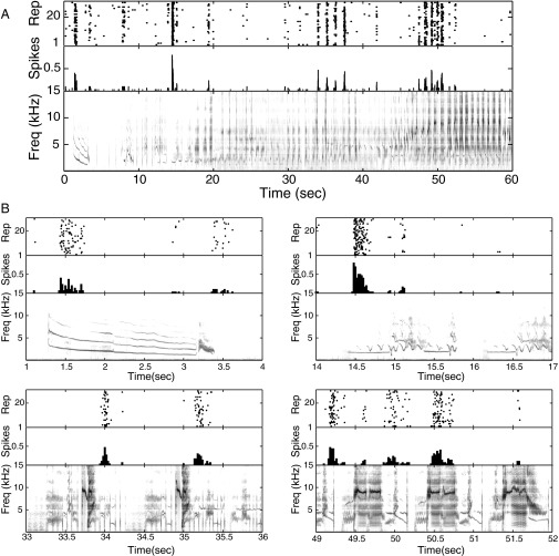
We recorded neuronal responses to six different 1-minute-long songs, each repeated 30 times. These songs were recorded from three male starlings, and together they contained over 200 motifs, brief segments of starling song that are perceived as distinct auditory objects (11). An NCM neuron usually responds to a variety of motifs (4, 12) (Fig. 1), and NCM neurons display rapid stimulus-specific adaptation (13), suggesting that an individual neuron can be sensitive to a variety of different stimulus features.

Fig. 1.

A single NCM neuron responds to several different motifs. (A) Spike raster plot (Top), peri-stimulus histogram (Middle), and spectrogram (Bottom) showing an example NCM neuron’s response to a full song. (B) Four 3-second-long excerpts taken at the indicated times from the response shown in A. The different panels show the neuron responding to acoustically distinct motifs (harmonic stacks, clicks, and other broadband stimuli), supporting the idea that individual NCM neurons can be sensitive to a variety of different stimulus features.

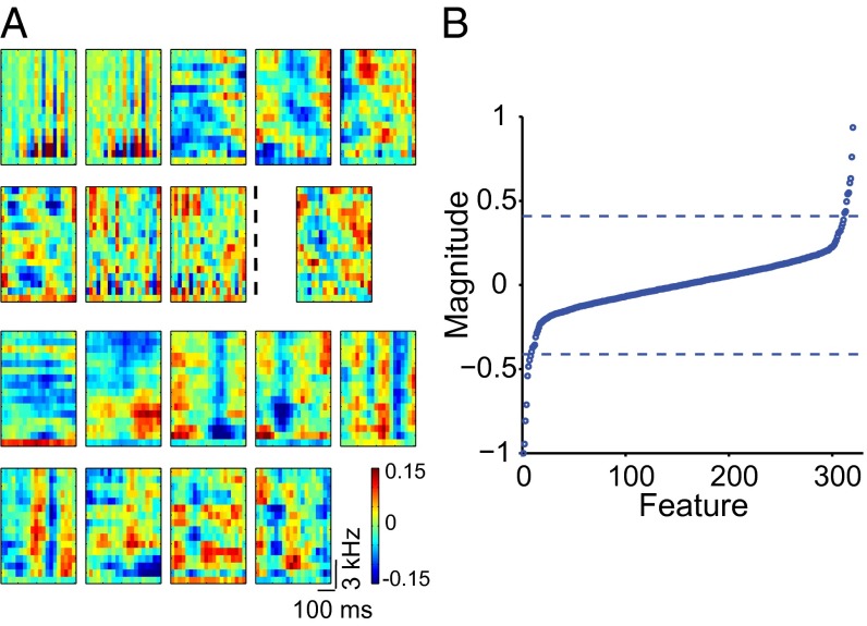
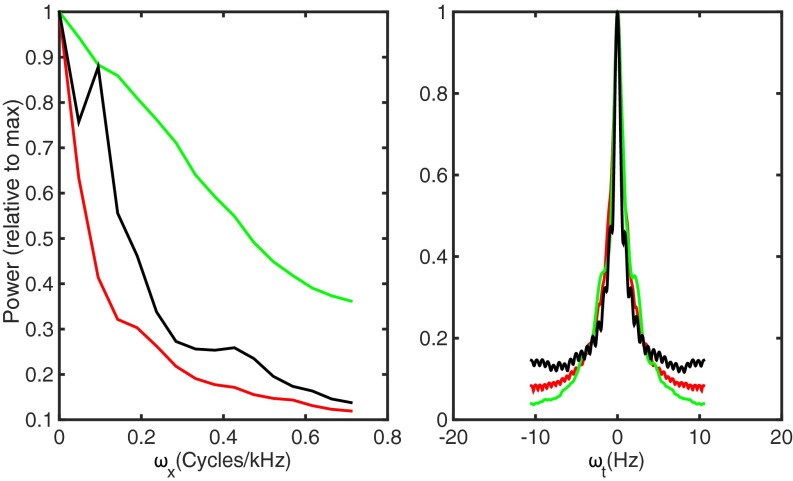
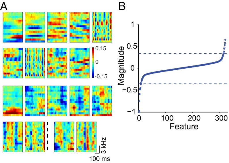
To examine whether single NCM neurons respond to multiple distinct features of starling song, we obtained significant eigenvectors of the second-order MNE model’s matrix J for each neuron that together with the first-order term (Methods) define its receptive field (Fig. 2). On average, NCM neurons’ receptive fields (n = 37 neurons) contained six excitatory features, or negative eigenvalues of the matrix J (6.43 ± 2.06, range 2–11, interquartile range 5–8), and six suppressive features, or positive eigenvalues of the matrix J (6.35 ± 2.41, range 3–12, interquartile range 5–7). As a control, we also determined the number of features using all possible five-song subsets of the six-song set. The distributions of significant features obtained using five or six songs were not statistically different (Kolmogorov–Smirnov test, P = 0.3 and P = 0.2 for the negative and positive eigenvalues, respectively). Using many more songs, however, did reveal additional features (see the next section). The features of each neuron’s receptive field were spectrotemporally diverse: the neurons typically combined broadband features resembling clicks and narrowband features resembling tones, or harmonic stacks. The spectral and temporal statistics of the ensemble of features were captured using the modulation power spectrum (14) (Fig. 3). Thus, we found multiple, distinct receptive-field features in individual high-level auditory neurons in response to natural stimuli. To reflect their multifeature composition, we call these receptive fields composite.

Fig. 2.

Composite receptive field of a single NCM neuron. (A) Examples of multiple excitatory and suppressive features obtained from one NCM neuron. The top two rows show the negative (excitatory) features. In this neuron, eight negative eigenvalues were significant. The largest nonsignificant eigenvector is also displayed to the right of the dotted line in row two and can be seen to contain structure. Eigenvectors corresponding to even smaller eigenvalues (not shown) contained no clear structure. The two bottom rows show nine significant positive (suppressive) features. (B) Eigenspectrum of the matrix J for the same neuron as in A. Eigenvalues were normalized for comparison with the data in Fig. 6B. The dashed lines indicate the two largest (in absolute value) positive and negative eigenvalues obtained from 500 symmetrical Gaussian random matrices with the same mean and variance as those of matrix J.

Fig. 3.

Capturing the statistics of feature ensembles. Projections of modulation power spectra for starling songs (green), MNE features (red), and artificial neural network features (black) on spectral (Left) and temporal (Right) axes.

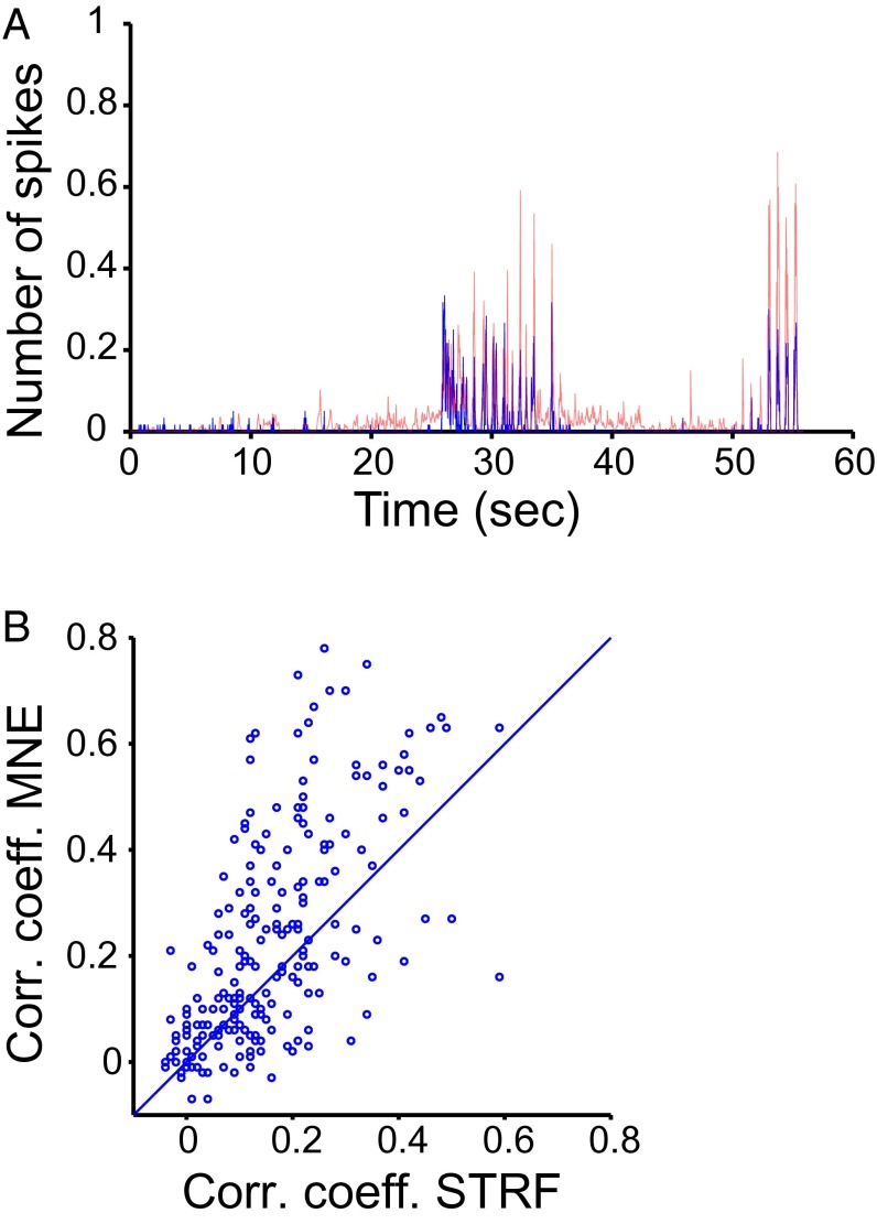
To verify the model’s ability to predict responses to new stimuli, we estimated its parameters for each neuron using all possible five-song subsets and generated a prediction of the probability of a spike for each time bin of each of the remaining songs (Methods). The correlation coefficients between the predicted and the measured responses ranged from zero (as not every song evoked a response in every neuron) to 0.8, with the average correlation of 0.23 ± 0.2 and the interquartile range of 0.06–0.36 (Fig. 4). Similar ranges of correlation values were reported using other methods (in particular, the Spectro-Temporal Receptive Field, or STRF) in the auditory forebrain of the zebra finch and starling (15, 16). To compare the two models (MNE and STRF) directly on our dataset, we obtained STRFs for all of the neurons in our sample using the widely used strfpak package (15). The STRF model provided significantly poorer predictions of responses to songs than the second-order MNE model (P = 1.4 × 10⁻⁵ with paired t test, Fig. 4B): the average correlation between the STRF prediction and the actual response was 0.16 ± 0.13, and the interquartile range was 0.06–0.23. Only 14 values (6%) obtained with the STRF model were equal or greater than 0.4, compared with four times as many (51 values, 23%) obtained with the MNE model. No correlation coefficients greater than 0.6 were obtained with the STRF model, whereas the MNE model produced 15 values greater than 0.6. Although the average values of the correlation coefficients indicate that both models are incomplete descriptions of the NCM neurons’ receptive fields, the MNE model revealed for the first time to our knowledge multiple receptive-field features in individual neurons responding to natural stimuli.

Fig. 4.

Prediction of responses to new stimuli. (A) The empirically measured time-varying average spike rate (blue) and the MNE-predicted spike rate (red) for a single neuron’s response to a song. The correlation coefficient between the measured and predicted response was 0.56. The number of spikes in each time bin was normalized by the number of stimulus repetitions. (B) Full distribution of correlation coefficients obtained with the second-order MNE model plotted against those obtained with the STRF. The diagonal line indicates unity.

Composite Receptive Fields Comprise Multiple Features of Similar Strength.

The function of the composite receptive fields must depend on the relative strength of component features. In this regard, it is noteworthy that eigenvalues of the matrix J, which defines feature strength, were of the same order of magnitude. For example, the average difference between the 10 largest (in absolute magnitude) neighboring negative eigenvalues, corresponding to excitatory features, of the neuron in Fig. 2 was 7%, and the maximal difference was 24%. Furthermore, many of the significant eigenvalues were small, i.e., at the border of significance, even though the associated eigenvectors contained clear structure (Fig. 2B). These observations imply that the auditory neurons’ receptive fields are not dominated by a single strong feature, but rather are characterized by a large number of somewhat weaker features of similar strength. These eigenvalue distributions contrast with those obtained using the same method from macaque retinal ganglion cells tuned to few features, where the difference between neighboring eigenvalues was several hundred percent, and from model cells with few built-in strong features corresponding to clearly outstanding eigenvalues (6). They are similar, however, to eigenvalue distributions obtained using a different method (STC) and an artificial stimulus—Gaussian noise flicker—in salamander retinal ganglion cells, which are known to be sensitive to multiple features (17).

One concern is that the observed similarities in feature strength reflect limits in the amount of data used to fit the model rather than the true properties of auditory neurons. To examine this possibility, we repeated the experiments and analyses using 60 1-minute-long songs, each repeated 10 times. We held some units with an excellent signal-to-noise ratio for 10 h or longer. We obtained features and eigenspectra from this 10-h dataset in five neurons (Fig. 5), four of which were also part of the main dataset (six songs repeated 30 times). The larger dataset allowed us to uncover some additional features in these neurons: in the same four neurons, we obtained 7.5 ± 2.1 negative and 7.5 ± 3.3 positive features with 6 songs, and 10.8 ± 1.3 negative and 8.3 ± 1.9 positive features with 60 songs (taking 40 among the 60 songs resulted in 10 ± 2.4 negative and 7.8 ± 1.7 positive features). To quantify similarity between features obtained with the two stimulus sets, we computed the correlation coefficient between each of the 6-song features and all of the features extracted from the 60-song dataset for that same neuron. Of the 54 features extracted from four neurons using the 6-song dataset, 35 had a correlation coefficient with a 60-song feature that was significantly greater than expected by chance (Methods), indicating they were preserved in the larger dataset. In addition, the mean similarity between features in the 6- and 60-song datasets from the same neuron was significantly higher than the similarity between datasets across neurons (P = 0.0011, paired t test). This supports the conclusion that large numbers of highly similar features are preserved between datasets from the same neuron and that these features primarily characterize properties of the neurons rather than the datasets used to obtain them. Moreover, the same characteristics of the eigenspectra persisted: eigenvalues of similar magnitude, with the average and maximal difference between the neighboring eigenvalues being 9% and 30%, and 8% and 15%, for the top 10 negative and positive eigenvalues, respectively (n = 5 neurons). Thus, the composite receptive fields of NCM neurons comprise multiple features of similar strength.

Fig. 5.

Composite receptive fields from larger datasets. (A) Examples of excitatory and suppressive features obtained from an NCM neuron using 60 1-minute-long songs. The top two rows show the nine significant excitatory features, and the two bottom rows show seven significant suppressive features. Two largest nonsignificant eigenvectors are also displayed (right-hand side of dotted line) and can be seen to contain structure and not only noise. (B) Eigenspectrum of the matrix J for the neuron in A. Eigenvalues were normalized for comparison with the data in Fig. 6B. The dashed lines indicate the two largest (in absolute value) positive and negative eigenvalues obtained from 500 symmetrical Gaussian random matrices with the same mean and variance as those of J.

Artificial Neural Network Reproduces These Receptive Fields Using Sparseness and Divisive Normalization.

We next examined whether receptive fields like those observed in NCM neurons could emerge through two encoding principles that have been proposed to be important to the function of neural circuits: sparseness and divisive normalization. Sparseness is a common property of cortical responses (18), where each neuron responds only to a small number of all stimuli (lifetime sparseness) and each stimulus activates only a small fraction of all neurons in the population (population sparseness). Divisive normalization, another general principle of neural computation (19), is the suppression or scaling of one neuron’s activity by the weighted activity in the circuit. We wondered whether an artificial neural network with the above constraints (sparseness and normalization) was able to learn composite receptive fields, with each unit pooling distinct features of similar strength, as observed in the biological neurons.

We trained a two-layer neural network using sparse filtering (20), a recently developed unsupervised learning algorithm (21), on the same 60 starling songs that we used to obtain the features in Fig. 5 and analyzed the acoustical features represented by units of this network. Because the principles (the cost function) that underlie the network’s features are well-understood and defined mathematically, the network can serve as a benchmark representation to which the biological neurons’ feature distributions can be compared.

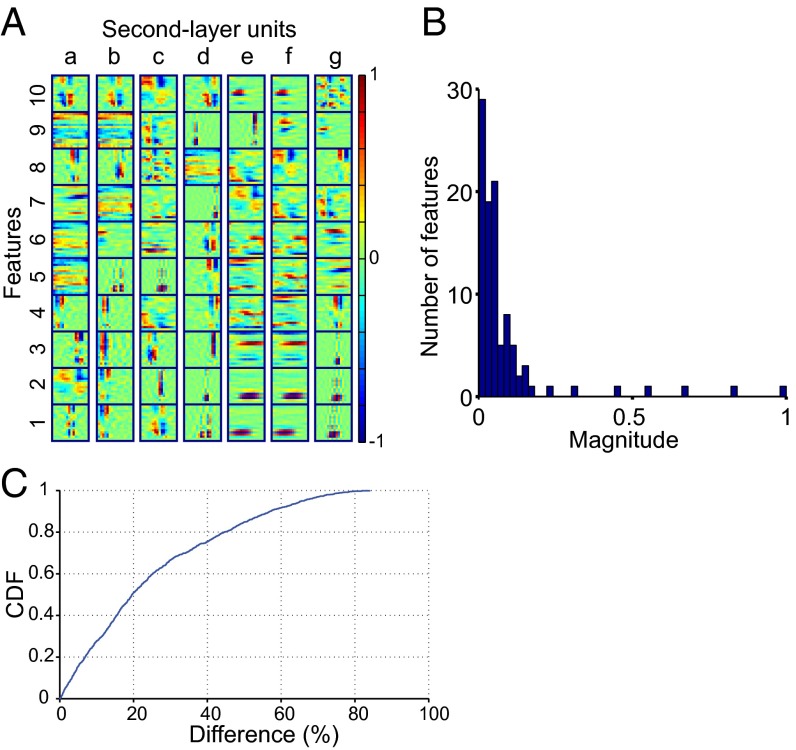
The network had two layers; the input layer (layer 1) learned basis features that resembled narrowband tones, broadband clicks, and some more complex structures. The second layer combined these features. Each layer-2 unit responded to several different first-layer features; that is, layer-2 units had composite receptive fields (Fig. 6A). Some layer-2 units had partially overlapping receptive fields. For example, the units “e” and “f” responded to the same (e.g., e1 and f1) as well as different (e.g., e9 and f9) features. This partially overlapping set of features was reminiscent of the mixture of precisely shared and independent receptive-field subregions in neighboring neurons in the mouse visual cortex (22). The population sparseness constraint assured that only a few basis features were active for each layer-2 unit; competition between units (normalization) assured that active features had similar magnitudes (Fig. 6 B and C). The average difference between pairs of neighboring units (after sorting all units according to their activity and selecting 10 layer-1 units with the largest magnitude for each layer-2 unit) was 25%, and the maximal difference was 84% (Fig. 6C). This result accords with the receptive fields of NCM neurons, in which a few significant eigenvalues had similar magnitude (Figs. 2B and 5B). The spectrotemporal characteristics captured by these sets of sparse, evenly strong features matched those observed in the real neurons and those present in the songs themselves (Fig. 3). Note that the neural network did not explicitly model the stimulus distribution, but rather reproduced its properties based on the sparseness and normalization constraints.

Fig. 6.

Neural network trained on starling songs learns composite receptive fields. (A) Ten most active features for seven randomly chosen layer-2 units (a to g). (B) A histogram showing a distribution of the basis features’ activities for one layer-2 unit. The absolute normalized magnitude is shown for comparison with the distributions of features’ magnitudes in Figs. 2B and 5B. Note that most features are close to zero (lifetime sparseness) and that the most active features are of the same order of magnitude, as expected. (C) Cumulative density function (CDF) showing the percentage difference in the pair-wise magnitude between neighboring most active features of all layer-2 units. Ten largest basis features are selected for each layer-2 unit and sorted according to their activity (magnitude), then the percent difference is taken between the neighboring values.

Discussion

We have shown that individual high-level auditory neurons in the starling forebrain possess composite receptive fields comprising up to a dozen or more independent features of similar magnitudes. We then rediscover the distributions of these component features in an artificial neural network using divisive normalization and sparseness, suggesting plausible biological mechanisms for this composite representation.

The observed diversity and magnitude of features that drive spiking responses in NCM neurons is hard to reconcile with the strictest notions of feature selectivity implied by linear receptive-field models and low-dimensional stimulus representations. We show that the spiking response of a single NCM neuron can be produced by any one of many independent features. Although problematic at the level of a single neuron considered in isolation, this encoding scheme could be advantageous at the neuronal ensemble level because it allows each neuron to participate in many different ensembles. Computational models suggest that ensembles composed of diverse receptive fields, such as those we observed here, are superior for encoding multidimensional stimuli compared with populations in which each neuron responds to only a single stimulus (23). Recently, we also showed that the logical rules underlying the combination of independent inputs in NCM neurons can vary as a function both of the inputs and the neuron’s state, sometimes reflecting an AND-like operation, sometimes an OR-like operation (13). Collectively, it appears that individual NCM neurons act as flexible logical gates operating in a high-dimensional feature space.

Given their benefits, composite receptive fields may be a fundamental property of sensory systems that flexibly map diverse, multidimensional stimuli onto different behaviors. In support of this notion, composite receptive fields have also been identified in high-order olfactory neurons in mammals and insects (24, 25). In the olfactory system, because the number of odorants and odors that an individual may experience is very large and their identity cannot be predicted a priori, random projections of mitral cells in the olfactory bulb to pyramidal neurons in the piriform cortex are considered a good unbiased starting point from which learning then carves the associative networks (24, 26). In contrast, olfactory circuits mediating responses to pheromones, which are conserved evolutionarily and highly species-specific, are precisely wired, and the associated receptive fields are specific (26). Like the space of possible odors, the learned vocal repertoires of starlings and many other songbirds are large and unpredictable. Each adult starling has several dozen distinct motifs in its repertoire, most of which are unique to that bird, and the behavioral significance of these signals varies according to the idiosyncratic life history of both the singer and each listener (1). It is noteworthy that in both the associative olfactory centers and in high-order auditory neurons the representation of multidimensional and unpredictable natural stimuli is associated with the presence of composite receptive fields. Functionally similar properties have also been identified in prefrontal cortex, where many neurons are tuned to mixtures of multiple task-related aspects, and this so-called “mixed selectivity” has been suggested to be a hallmark of brain structures involved in cognition (27).

We also demonstrate how the observed composite receptive fields could emerge in sensory networks. Both the neural network trained in this study and the neurons in the starlings’ brains display receptive fields that capture the statistics of the starling song. Unsupervised learning algorithms in general can produce statistically optimal representations of complex inputs (28, 29) and have been used successfully to model simple-cell receptive fields in primary visual cortex (30) and auditory responses in the cochlear nerve (31). The success of both these efficient sensory encoding models is directly based on the maximization of sparseness in the underlying algorithms. We show that the same constraint of sparseness, coupled with divisive normalization between units within each network layer, yields representations with receptive fields composed of several distinct features of similar magnitude. Thus, these processes may be general constraints that shape information processing across multiple neuronal stages. A key question for future research is to understand both the implementation of sparseness (18) and normalization in sensory neural circuits and the functional significance of discontinuous, composite, and apparently random receptive fields in songbirds and other animals. The success of random projections for dimensionality reduction, e.g., in compressed sensing and machine learning (32–34), provides useful frameworks for this research.

Methods

Spike Recording and Sorting.

Under a protocol approved by the Institutional Animal Care and Use Committee of the University of California, San Diego, we performed experiments on adult male European starlings (Sturnus vulgaris). We obtained stimuli for the experiments by recording songs from adult male starlings (unfamiliar to the test subjects) inside a sound attenuation box (Acoustic Systems) at 44.1 thousand samples/s. For physiological testing, birds were anesthetized (urethane, 7 mL·kg⁻¹) and head-fixed to a stereotaxic apparatus mounted inside a sound attenuation box. The use of urethane was necessary to obtain the long-stimulus presentation epochs required in this study and is unlikely to alter selectivity significantly (15, 16). Songs were played to the subjects at 60-dB mean-level while we recorded action potentials extracellularly using 32-channel electrode arrays (NeuroNexus Technologies) inserted through a small craniotomy into the NCM. Stimulus presentation, signal recording, and spike sorting were controlled through a PC using Spike2 software (CED). Extracellular voltage waveforms were amplified (model 3600 amplifier, A-M Systems), filtered, and sampled with a 50-µs resolution and saved for offline spike sorting. Single units were identified by clustering principle components of the spike waveforms, only when no violations of the refractory period (assumed to equal 1 ms) occurred, and only from recordings with an excellent signal-to-noise ratio (large-amplitude extracellular action-potential waveforms). All analyses, except for spike sorting, were performed in Matlab (MathWorks).

MNE Receptive-Field Analysis.

To compute the linear and quadratic features, we downsampled stimuli to 24 kHz and converted them into spectrograms using spectrogram function in Matlab with parameters: nfft = 128, Hanning window of length 128, and a 50% segment overlap. The DC component was removed, and the adjacent 64 frequencies were averaged pair-wise twice to obtain 16 frequency bands ranging from 750 Hz to the Nyquist frequency (12 kHz). The adjacent time bins were averaged three times for a final bin size of 21 ms. We typically used 20 time bins to compute MNE receptive fields (both the linear and quadratic features). Using stimuli with 32 instead of 16 frequencies, or smaller time bins, or a different number of time bins (10, 16, 32) to compute receptive fields gave similar results. The spectrograms were converted into the logarithmic scale.

A full description of the MNE model is given in ref. 6. Briefly, the minimal model describes the probability of a spike, given a stimulus s (e.g., a song spectrogram), as $P(spike|s)=(1+\exp {(a+sh+s^{T}Js)}^{-1}$, which is a logistic function with parameters a, h, and J determined to satisfy the mean firing rate and the correlations with the first and second moments of the stimulus, respectively (6). Data were divided into two sets for training and testing; the testing set contained one-quarter of the data. Parameters were estimated four times, each time using a different segment of data for training and testing, and averaged. Early stopping was used for regularization to prevent overfitting. As in STC, diagonalizing the matrix J yields quadratic features with the same time and frequency dimensions as the original stimuli that drove spiking. To test significance, the eigenvalues of J were compared with those obtained from a randomly reshuffled J matrix. As a second test of the eigenvalues’ significance, we constructed 500 symmetrical Gaussian random matrices with the same mean and variance as those of J and obtained a distribution of their eigenvalues. Eigenvalues of J were considered significant if they were outside of this distribution. The two approaches resulted in the same, or similar, numbers of significant eigenvalues. When the numbers were not the same (and they never differed by more than 1), we conservatively chose the smaller number.

To test how well the model predicted responses to new stimuli, we obtained the parameters a, h, and J for each neuron using all subsets of five among the six songs and generated a prediction of the response to the remaining sixth song not used in the parameter estimation. This prediction was then compared with the actual response to that song using the Matlab corrcoef function.

Feature Similarity.

For a subset of neurons, we computed the correlation coefficient (CC) between each feature extracted from the 6-song dataset and each feature extracted from the 60-song dataset for that same neuron. We count a 6-song feature as “preserved” in the larger dataset if the correlation coefficient between it and any feature in the 60-song set exceeds the bounds of the 95% confidence for all CCs between 6-song and 60-song features from that neuron. We quantified feature similarity directly by computing the absolute value of the correlation coefficient between each of the 54 features from the 6-song dataset and each of the 73 features from the 60-song datasets for all neurons in which they were obtained (n = 4). We used the absolute value of the CC because the features are quadratic; the same feature can appear in different datasets as spectrograms with opposite polarity (i.e., with the red and the blue regions reversed). We considered the CC with the largest absolute value among all of the features from the 60-song dataset from the same neuron to be the best within-cell match and the average of the CCs with the largest absolute value among the features in each of the 60-song datasets obtained from different cells to be the best between-cell match. We then compared the best within-cell match to the best between-cell match for each six-song feature using a paired t test. Although our analysis shows that similar features are maintained across datasets from the same cell, both the preservation of (comparatively stronger) features and the loss of (comparatively weaker) features are expected as songs from new birds are added. Because all features are not independent and must be orthogonal, if a new strong feature appears that is not orthogonal to an existing weak feature, the weak feature will change. As more data are added, the basis vectors have to change to remain orthogonal.

Unsupervised Neural Network.

The network was forced to construct a compact representation of starling song by learning features based on the song statistics and subject to two constraints. First, only a small fraction of units should be active at any time (population sparseness). Second, all units should compete with each other and therefore be approximately equally active (high dispersal). As a result of this competition—akin to divisive normalization in neural circuits—in conjunction with the population sparseness constraint, any individual unit was active only rarely (lifetime sparseness). These three characteristics—population sparseness, lifetime sparseness, and normalization—are typical of neuronal activity in the cortex. To implement the network, we used the code from Ngiam et al. (2011) (20), which is freely available. Briefly, the sparse filtering objective (eq. 1 in ref. 20) first normalizes features by dividing them by their L2-norm over all training examples to assure that they are equally active and lie on the unit L2-ball (a sphere of unit radius), and then the algorithm minimizes the L1-norm of the normalized features over the set of examples to optimize for sparseness. Ngiam et al. (2011) (20) provide a detailed description. The algorithm has only one hyperparameter, the number of features to learn. We tried values between 100 and 256 for both layers and consistently obtained the same features; the final results were obtained with 100 target features. The first layer was trained on starling songs converted into log-spectrograms. The second layer was trained on the normalized first-layer features, using a greedy layer-wise stacking commonly used in deep neural architectures (35).

References

- 1.Eens M. Understanding the complex song of the European starling: An integrated ethological approach. Adv Stud Behav. 1997;26:355–434. [Google Scholar]
- 2.Butler AB, Reiner A, Karten HJ. Evolution of the amniote pallium and the origins of mammalian neocortex. Ann N Y Acad Sci. 2011;1225:14–27. doi: 10.1111/j.1749-6632.2011.06006.x. [DOI] [PMC free article] [PubMed] [Google Scholar]
- 3.Theunissen FE, Shaevitz SS. Auditory processing of vocal sounds in birds. Curr Opin Neurobiol. 2006;16(4):400–407. doi: 10.1016/j.conb.2006.07.003. [DOI] [PubMed] [Google Scholar]
- 4.Thompson JV, Gentner TQ. Song recognition learning and stimulus-specific weakening of neural responses in the avian auditory forebrain. J Neurophysiol. 2010;103(4):1785–1797. doi: 10.1152/jn.00885.2009. [DOI] [PMC free article] [PubMed] [Google Scholar]
- 5.Schneider DM, Woolley SMN. Sparse and background-invariant coding of vocalizations in auditory scenes. Neuron. 2013;79(1):141–152. doi: 10.1016/j.neuron.2013.04.038. [DOI] [PMC free article] [PubMed] [Google Scholar]
- 6.Fitzgerald JD, Rowekamp RJ, Sincich LC, Sharpee TO. Second order dimensionality reduction using minimum and maximum mutual information models. PLOS Comput Biol. 2011;7(10):e1002249. doi: 10.1371/journal.pcbi.1002249. [DOI] [PMC free article] [PubMed] [Google Scholar]
- 7.Jaynes E. Information theory and statistical mechanics. Phys Rev. 1957;106(4):620–630. [Google Scholar]
- 8.Globerson A, Stark E, Vaadia E, Tishby N. The minimum information principle and its application to neural code analysis. Proc Natl Acad Sci USA. 2009;106(9):3490–3495. doi: 10.1073/pnas.0806782106. [DOI] [PMC free article] [PubMed] [Google Scholar]
- 9.Steveninck RDRV, Bialek W. Real-time performance of a movement-sensitive neuron in the blowfly visual system: Coding and information transfer in short spike sequences. Proc R Soc B Biol Sci. 1988;234(1277):379–414. [Google Scholar]
- 10.Sharpee T, Rust NC, Bialek W. Analyzing neural responses to natural signals: Maximally informative dimensions. Neural Comput. 2004;16(2):223–250. doi: 10.1162/089976604322742010. [DOI] [PubMed] [Google Scholar]
- 11.Gentner TQ. Temporal scales of auditory objects underlying birdsong vocal recognition. J Acoust Soc Am. 2008;124(2):1350–1359. doi: 10.1121/1.2945705. [DOI] [PMC free article] [PubMed] [Google Scholar]
- 12.Meliza CD, Margoliash D. Emergence of selectivity and tolerance in the avian auditory cortex. J Neurosci. 2012;32(43):15158–15168. doi: 10.1523/JNEUROSCI.0845-12.2012. [DOI] [PMC free article] [PubMed] [Google Scholar]
- 13.Kozlov AS, Gentner TQ. Central auditory neurons display flexible feature recombination functions. J Neurophysiol. 2014;111(6):1183–1189. doi: 10.1152/jn.00637.2013. [DOI] [PMC free article] [PubMed] [Google Scholar]
- 14.Elliott TM, Theunissen FE. The modulation transfer function for speech intelligibility. PLOS Comput Biol. 2009;5(3):e1000302. doi: 10.1371/journal.pcbi.1000302. [DOI] [PMC free article] [PubMed] [Google Scholar]
- 15.Theunissen FE, Sen K, Doupe AJ. Spectral-temporal receptive fields of nonlinear auditory neurons obtained using natural sounds. J Neurosci. 2000;20(6):2315–2331. doi: 10.1523/JNEUROSCI.20-06-02315.2000. [DOI] [PMC free article] [PubMed] [Google Scholar]
- 16.Meliza CD, Chi Z, Margoliash D. Representations of conspecific song by starling secondary forebrain auditory neurons: Toward a hierarchical framework. J Neurophysiol. 2010;103(3):1195–1208. doi: 10.1152/jn.00464.2009. [DOI] [PMC free article] [PubMed] [Google Scholar]
- 17.Fairhall AL, et al. Selectivity for multiple stimulus features in retinal ganglion cells. J Neurophysiol. 2006;96(5):2724–2738. doi: 10.1152/jn.00995.2005. [DOI] [PubMed] [Google Scholar]
- 18.Babadi B, Sompolinsky H. Sparseness and expansion in sensory representations. Neuron. 2014;83(5):1213–1226. doi: 10.1016/j.neuron.2014.07.035. [DOI] [PubMed] [Google Scholar]
- 19.Carandini M, Heeger DJ. Normalization as a canonical neural computation. Nat Rev Neurosci. 2012;13(1):51–62. doi: 10.1038/nrn3136. [DOI] [PMC free article] [PubMed] [Google Scholar]
- 20.Ngiam J, Chen Z, Bhaskar SA, Koh PW, Ng AY. Sparse filtering. Adv Neural Inf Process Syst. 2011;24:1125–1133. [Google Scholar]
- 21.Goodfellow IJ, et al. 2015. Challenges in representation learning: A report on three machine learning contests Neural Networks 64(59–63)
- 22.Smith SL, Häusser M. Parallel processing of visual space by neighboring neurons in mouse visual cortex. Nat Neurosci. 2010;13(9):1144–1149. doi: 10.1038/nn.2620. [DOI] [PMC free article] [PubMed] [Google Scholar]
- 23.Sánchez-Montañés MA, Pearce TC. Why do olfactory neurons have unspecific receptive fields? Biosystems. 2002;67(1-3):229–238. doi: 10.1016/s0303-2647(02)00081-3. [DOI] [PubMed] [Google Scholar]
- 24.Stettler DD, Axel R. Representations of odor in the piriform cortex. Neuron. 2009;63(6):854–864. doi: 10.1016/j.neuron.2009.09.005. [DOI] [PubMed] [Google Scholar]
- 25.Caron SJ, Ruta V, Abbott LF, Axel R. Random convergence of olfactory inputs in the Drosophila mushroom body. Nature. 2013;497(7447):113–117. doi: 10.1038/nature12063. [DOI] [PMC free article] [PubMed] [Google Scholar]
- 26.Miyamichi K, et al. Cortical representations of olfactory input by trans-synaptic tracing. Nature. 2011;472(7342):191–196. doi: 10.1038/nature09714. [DOI] [PMC free article] [PubMed] [Google Scholar]
- 27.Rigotti M, et al. The importance of mixed selectivity in complex cognitive tasks. Nature. 2013;497(7451):585–590. doi: 10.1038/nature12160. [DOI] [PMC free article] [PubMed] [Google Scholar]
- 28.Bhand M, Mudur R, Suresh B, Saxe A, Ng AY. Unsupervised learning models of primary cortical receptive fields and receptive field plasticity. Adv Neural Inf Process Syst. 2011;24:1971–1979. [Google Scholar]
- 29.Le Q, et al. 2012. Building high-level features using large scale unsupervised learning. 29th International Conference on Machine Learning. Available at icml.cc/2012/papers/73.pdf. Accessed January 13, 2016.
- 30.Olshausen BA, Field DJ. Emergence of simple-cell receptive field properties by learning a sparse code for natural images. Nature. 1996;381(6583):607–609. doi: 10.1038/381607a0. [DOI] [PubMed] [Google Scholar]
- 31.Smith EC, Lewicki MS. Efficient auditory coding. Nature. 2006;439(7079):978–982. doi: 10.1038/nature04485. [DOI] [PubMed] [Google Scholar]
- 32.Candes EJ, Tao T. Near-optimal signal recovery from random projections: Universal encoding strategies? IEEE Trans Inf Theory. 2006;52(12):5406–5425. [Google Scholar]
- 33.Blum A. In: Subspace, Latent Structure and Feature Selection. Saunders C, et al., editors. Springer; Berlin: 2006. [Google Scholar]
- 34.Allen-Zhu Z, Gelashvili R, Micali S, Shavit N. Sparse sign-consistent Johnson-Lindenstrauss matrices: Compression with neuroscience-based constraints. Proc Natl Acad Sci USA. 2014;111(47):16872–16876. doi: 10.1073/pnas.1419100111. [DOI] [PMC free article] [PubMed] [Google Scholar]
- 35.Hinton GE, Salakhutdinov RR. Reducing the dimensionality of data with neural networks. Science. 2006;313(5786):504–507. doi: 10.1126/science.1127647. [DOI] [PubMed] [Google Scholar]