Enhanced, targeted sampling of high-dimensional free-energy landscapes using variationally enhanced sampling, with an application to chignolin

Significance

The problem of sampling complex systems characterized by metastable states separated by kinetic bottlenecks is a universal one that has received much attention. Popular strategies involve applying a bias to a small number of collective variables. This strategy fails when the choice of collective variable is not clear or when the system’s free energy cannot be projected meaningfully on a low-dimensional manifold. We use a variational principle that allows one to construct approximate but effective multidimensional biases. We show in a practical case that the method is much more efficient than alternative methods. We expect this method to be useful for a wide variety of sampling problems in chemistry, biology, and materials science.

Abstract

The capabilities of molecular simulations have been greatly extended by a number of widely used enhanced sampling methods that facilitate escaping from metastable states and crossing large barriers. Despite these developments there are still many problems which remain out of reach for these methods which has led to a vigorous effort in this area. One of the most important problems that remains unsolved is sampling high-dimensional free-energy landscapes and systems that are not easily described by a small number of collective variables. In this work we demonstrate a new way to compute free-energy landscapes of high dimensionality based on the previously introduced variationally enhanced sampling, and we apply it to the miniprotein chignolin.

Molecular simulation has become an increasingly useful tool for studying complex transformations in chemistry, biology, and materials science. Such simulations provide extremely high spatial and temporal resolution but suffer from inherent time-scale limitations. Molecular dynamics simulations of biomolecules performed on standard hardware struggle to exceed the microsecond time scale. Modern, purpose-built hardware can reach the millisecond time scale (1), but these tools are not generally available and they still prove insufficient for many important problems (2). Widely used enhanced sampling methods also allow one to simulate processes with a time scale of milliseconds (3) and there is significant interest in extending these methods. One important class of enhanced sampling methods involves applying an external bias to one or more collective variables (CVs) of the system. Umbrella sampling and metadynamics fall into this category (4, 5), but there are many other examples (6–13). These methods are most effective when the transformations of interest are in some sense collective and can be described by a very small number of CVs.

When the choice of CV is not obvious or the free-energy landscape cannot be projected meaningfully on a low-dimensional manifold, new strategies are needed. Here we describe an enhanced sampling strategy that allows one to bias high-dimensional free-energy landscapes by exploiting the flexibility inherent in the recently introduced variationally enhanced sampling (VES) method (14). This method casts free-energy computation as a functional minimization problem, and it solves two important problems associated with high-dimensional free-energy computation. The first problem is that when exploring a high-dimensional space a system might never visit the regions of interest, but the variational principle introduced in ref. 14 permits us to specifically target the region we are interested in through the use of a so-called “target distribution.” The second problem is that one must adopt an approximation for the high-dimensional bias and the variational principle allows us to do this in an optimal way. Furthermore, as we show here, for the first time to our knowledge, choosing an intelligent target distribution, which includes any available a priori information, allows us to compensate for some of the variational flexibility that is lost when we adopt an approximate form for the bias. We apply this method to study the folding and unfolding of chignolin and show that we can accurately estimate the folding free energy in a small fraction of the computational time used by other methods.

Background

To put our method in context we will provide some background on the methods that have been explored for overcoming barriers in high-dimensional CV spaces. Most of these methods involve applying an external bias to some CVs of the system. Standard methods like metadynamics and umbrella sampling are effective for low-dimensional CV spaces and they achieve the dual goal of allowing the system to explore the CV space and reconstructing the free-energy surface accurately. Methods that attempt to sample high-dimensional CV spaces often sacrifice the second goal. Bias-exchange metadynamics (15), for example, biases a different CV in each of several replicas and then allows exchange moves between replicas. The output of such a calculation is several one-dimensional representations of the free-energy surface on each of the biased CVs. A related method is the recently introduced parallel bias metadynamics, which also produces many low-dimensional free-energy surfaces but eliminates the exchange moves (16). Methods like replica exchange with CV tempering (17) and biasing potential replica exchange molecular dynamics (18) rely on a replica exchange scheme to collect statistics from an unbiased replica, and they use either a predefined or an iteratively constructed bias to help the system explore in biased replicas which can exchange with the unbiased replica. An alternative approach is to use some machine learning procedure to identify the important basins in a high-dimensional space, as is done in reconnaissance metadynamics (19) or in ref. 20. Other methods do without an external bias altogether, like temperature-accelerated molecular dynamics (MD) (21), in which an artificially large friction is applied to a set of CVs to ensure that they evolve slowly compared with the atomic motions. This list is by no means exhaustive; for a more thorough review see for example ref. 22, but the sheer number of attempts to solve this problem testifies to its importance.

Algorithm

The VES approach was introduced by Valsson and Parrinello in ref. 14 and extensions have been described in refs. 23, 24. In this approach the system is biased by a potential $V\left(\mathbf{s}\right)$, which acts on a set of CVs $\mathbf{s}=\left(s_1,\dots ,s_d\right)$ and which is updated over the course of the simulation to minimize a functional $\mathrm{\Omega }\left[V\right]$:

$$\mathrm{\Omega }\left[V\right]=\frac{1}{\beta }\log \frac{{\displaystyle \int d\mathbf{s}\hspace{0.17em}{e}^{-\beta \left[F\left(\mathbf{s}\right)+V\left(\mathbf{s}\right)\right]}}}{{\displaystyle \int ds\hspace{0.17em}{e}^{-\beta F\left(\mathbf{s}\right)}}}+{\displaystyle \int d\mathbf{s}\hspace{0.17em}p\left(\mathbf{s}\right)V\left(\mathbf{s}\right)},$$ [1]

where $\beta =1/k_{\text{B}}T$ and $F\left(\mathbf{s}\right)$ is the free-energy surface corresponding to the set of CVs. $p\left(\mathbf{s}\right)$ in this expression is known as the target distribution and it can be either predefined or determined by some iterative procedure during the simulation (23, 24). As we will see, the target distribution is the distribution that the biased system samples in the long time limit and thus it allows one to emphasize which states one wishes to sample. This is distinct, however, from choosing a particular configuration and biasing the system toward that configuration. The $V\left(\mathbf{s}\right)$ that minimizes this functional obeys the relationship

$$V\left(\mathbf{s}\right)=-F\left(\mathbf{s}\right)-\frac{1}{\beta }\text{log}\hspace{0.17em}p\left(\mathbf{s}\right)+C,$$ [2]

where C is an unimportant constant. In an ergodic simulation biased by $V\left(\mathbf{s}\right)$, the CVs sample the distribution $P_V\left(\mathbf{s}\right)\propto e^{-\beta \left[F\left(\mathbf{s}\right)+V\left(\mathbf{s}\right)\right]}$ and we see that $P_V\left(\mathbf{s}\right)=p\left(\mathbf{s}\right)$ when the minimum is reached. The functional $\mathrm{\Omega }\left[V\right]$ is convex with respect to $V\left(\mathbf{s}\right)$ which means that this is the global minimum. Minimizing this functional is equivalent to minimizing the Kullback–Leibler divergence between the sampled distribution and the target distribution (25–28). Eqs. 1 and 2 define the variational principle that we make use of in this paper.

To perform the minimization of $\mathrm{\Omega }\left[V\right]$ it is generally most convenient to expand $V\left(\mathbf{s}\right)$ in a set of basis functions

$$V\left(\mathbf{s};\mathit{\alpha }\right)={\displaystyle \sum _k{\alpha }_k{f}_k\left(\mathbf{s}\right)},$$ [3]

for example, plane waves or products of Chebyshev polynomials, and use the set of expansion coefficients ${\alpha }_k$ as variational parameters. The approach we use to minimize $\mathrm{\Omega }$ with respect to these parameters is identical to the approach described in ref. 14, and it is based on the stochastic optimization method from ref. 29. We provide a detailed description in the Supporting Information.

As a prototypical example of a high-dimensional free-energy surface, we will consider the backbone dihedral angles of a protein. In particular, we will study chignolin, a small 10-residue-long protein. It must be said, however, that our method is completely general and after appropriate adaptation it could be applied to many other problems such as, for instance, nucleation and ligand binding. The advantage of studying chignolin is that its experimental structure is known (30) and it has been simulated for 100 μs using a special purpose machine (1), in addition to many other simulation studies (e.g., refs. 31–33), which provides us with good reference data. In ref. 1 chignolin was studied very close to the folding temperature, and a folding time of $\approx$0.6 μs and an unfolding time of $\approx$2.2 μs were measured. These time scales put the study of this protein outside the range of ordinary MD simulations on standard hardware.

A complete characterization of the ensemble of conformations of chignolin would require calculating the free energy as a function of all of its backbone dihedral angles. In general there are two highly flexible dihedral angles per residue, ϕ and ψ, with a few exceptions like proline in which only the ψ angle can truly rotate, and the N-terminal and C-terminal residues which only have one flexible dihedral angle. For simplicity we will refer to the set of N biased dihedral angles as ${\theta }_i$. In total there are 17 dihedral angles that determine the structure of chignolin, which means that a straightforward calculation of the free-energy surface is clearly impossible and also finding a restricted number of CVs capable of describing the conformational manifold is challenging. Thus, to solve this multidimensional problem we shall use an approximate but computationally tractable expression for $V\left(\mathbf{s}\right)$, where $\mathbf{s}$ is the set of 17 dihedral angles. This is in spirit very similar to what is done in quantum chemistry when deriving the Hartree–Fock equations (34). Namely, it is first assumed that the wave function has the form of a single Slater determinant. Then use is made of the Rayleigh–Ritz variational principle to derive the equations whose solution will give the optimal determinant.

In our case however we can add to the power of the variational principle the flexibility that comes from the freedom of choosing the target distribution $p\left(\mathbf{s}\right)$. To better understand this point let us consider the case in which $p\left(\mathbf{s}\right)$ is the equilibrium distribution $p\left(\mathbf{s}\right)=\text{exp}\left[-\beta F\left(\mathbf{s}\right)\right]/Z$. In such a case the functional is minimum for $V\left(\mathbf{s}\right)=0$ and $F\left(\mathbf{s}\right)=-\left(1/\beta \right)\log p\left(\mathbf{s}\right)$ if we ignore irrelevant constants. Of course $F\left(\mathbf{s}\right)$ is the very quantity we want to evaluate and it is not available but we can imagine having an approximation $F_o\left(\mathbf{s}\right)=-\left(1/\beta \right)\log p\left(\mathbf{s}\right)$ and in this case at the minimum the variational principle gives

$$F\left(\mathbf{s}\right)=-V\left(\mathbf{s}\right)+F_o\left(\mathbf{s}\right).$$ [4]

This equation is equivalent to Eq. 2 but it has been recast in a form that allows one to view the bias $V\left(\mathbf{s}\right)$ as the correction to the initial estimate. There is a conceptual as well as a technical consequence of this observation. From a conceptual point of view, sampling can be greatly accelerated with an adroit choice of $p\left(\mathbf{s}\right)$ that captures as much as possible any a priori information we have on the system. From a technical point of view the requirements on the variational flexibility are much less stringent because $V\left(\mathbf{s}\right)$ only needs to correct the errors in $F_o\left(\mathbf{s}\right)$, especially those errors around the minimum. Thus, even an approximate form of $V\left(\mathbf{s}\right)$ can still be capable of correcting $F_o\left(\mathbf{s}\right)$.

Let us illustrate this point on chignolin. This small protein free-energy landscape is characterized by two basins, the folded state and the unfolded one. In the first, the protein is folded in a structure that can be described by a set of dihedral angles ($\overline{{\theta }_i}$) about which the protein oscillates. The other basin is the unfolded ensemble in which no definite stable structure can be identified. Thus, to assist sampling we construct a $p\left(\mathbf{s}\right)$ that reflects these two features. We write $p\left(\mathbf{s}\right)$ as a sum of two contributions:

$$p\left(\mathbf{s}\right)=w_f{p}_f\left(\mathbf{s}\right)+w_u{p}_u\left(\mathbf{s}\right),$$ [5]

where the positive weights, $w_f$ and $w_u$, are such that $w_f+w_u=1$, and $p_f\left(\mathbf{s}\right)$ and $p_u\left(\mathbf{s}\right)$ are distributions that describe the folded state and the unfolded state, respectively. In building $p_f\left(\mathbf{s}\right)$ and $p_u\left(\mathbf{s}\right)$ we have to keep in mind that it is computationally advantageous to be able to easily calculate the term ${\langle f_i\left(\mathbf{s}\right)\rangle }_{p\left(\mathbf{s}\right)}$ which appears on the right-hand side of Eq. S1. Possibly the simplest $p_f\left(\mathbf{s}\right)=p_f\left({\theta }_1,\dots ,{\theta }_N\right)$ that satisfies these requirements is obtained by writing $p_f\left({\theta }_1,\dots ,{\theta }_N\right)$ as a product of functions localized around the reference angles $\overline{{\theta }_i}$. The von Mises function, which is the periodic analog of the Gaussian function, lends itself to this use. This leads to

$$p_f\left(\mathbf{s}\right)=p_f\left({\theta }_1,\dots ,{\theta }_N\right)={\mathrm{\Pi }}_i\frac{e^{\kappa \text{cos}\left({\theta }_i-{\overline{\theta }}_i\right)}}{2\pi I_0\left(\kappa \right)},$$ [6]

where $I_0\left(\kappa \right)$ is the modified Bessel function of order zero and each function in the product is localized around ${\overline{\theta }}_i$ and has variance $1/\kappa$. We have chosen $\kappa =5$, which corresponds roughly to the magnitude of fluctuations in the folded state. To assist sampling of the unfolded state we simply use the uniform distribution:

$$p_u\left({\theta }_1,\dots ,{\theta }_N\right)=\frac{1}{{\left(2\pi \right)}^N}.$$ [7]

If the relative size of the two basins is known one could choose the weights accordingly. For instance, based on the results from ref. 1 one could have chosen $w_f=2/3$ and $w_u=1/3$ to better reflect their results. However, to show the robustness of our procedure we have made the blind choice $w_f=w_u=1/2$. In what follows, we will discuss briefly how different choices of $w_f$ and $w_u$ can affect the rate of convergence and the sampling.

The next step is to simplify the expression for the multidimensional $V\left(\mathbf{s}\right)$. In this work we express the bias as the sum of two body biases where only dihedrals that are next-nearest neighbors along the peptide chain are explicitly correlated:

$$V\left({\theta }_1,\dots ,{\theta }_N\right)\approxeq V_1\left({\theta }_1,{\theta }_2\right)+V_2\left({\theta }_2,{\theta }_3\right)+\dots V_{N-1}\left({\theta }_{N-1},{\theta }_N\right),$$ [8]

where each term is expanded as in Eq. 2. This form is inspired by the Ising model and takes advantage of the linear structure of the protein. The long-range correlations that are not explicitly taken into account are introduced indirectly through our choice of $p\left(\mathbf{s}\right)$. This model does assume that long-range correlations are negligible when the protein is not near the folded state. This may seem like a severe approximation but recent work has demonstrated that an optimal causality model for the Ala-10 peptide only includes correlations that are local in time and space (35). The computational advantages of this form are evident. If we let M be the size of the basis set that is needed to express the angular dependence of each individual dihedral angle, then the number of basis functions required to represent the left-hand side above is $M^{17}$ whereas the number of basis functions required to represent the approximate right-hand side is reduced to manageable $16M^2$.

Results

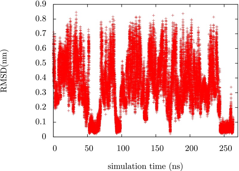
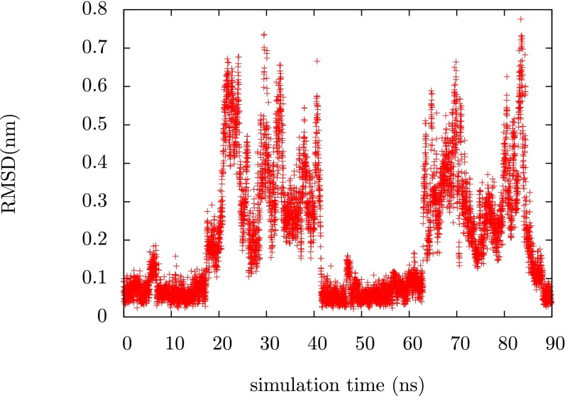
Fig. 1 shows a time series of the root-mean-square displacement (RMSD) from the folded state reference structure for chignolin. This time series was taken from a simulation in which the bias was being optimized to sample the target distribution described above and it shows the protein going back and forth between folded and unfolded states. The protein was initiated in an extended state but in less than 300 ns we see at least four transitions between the unfolded state and the folded state. The ability to generate these transitions underlies any study of the folding transition, whether they be studies of thermodynamics or kinetics. In the Supporting Information we demonstrate that the bias converges over this time scale, indicating that the functional $\mathrm{\Omega }\left[V\right]$ has been minimized with respect to the variational parameters. This behavior is somewhat sensitive to the exact choice of $w_f$ and $w_u$. In fact, one of the main results of the paper is to illuminate the role that $p\left(\mathbf{s}\right)$ can have in assisting and guiding sampling. If we choose $w_f=0$ (which is just targeting a uniform distribution in the dihedral angles), we find that the system explores the unfolded state thoroughly but never finds the folded state. Higher values of $w_f$ can assist the system in finding the folded state faster. In the Supporting Information we show a time series for $w_f=0.85$ and we see that in this case the rate of folding is faster.

Fig. 1.

Time series of the Cα RMSD from the reference structure for chignolin during the optimization process. We see several transitions between the folded and the unfolded state of the protein.

This approach gives us various ways to study the physics of chignolin. One interesting possibility involves examining the high-dimensional free-energy surface itself. In the present study, however, we will focus on extracting information from the unbiased ensemble on CVs that we have not directly biased. Recovering this information directly from the optimization simulations can be a difficult reweighting problem. One simple way to sidestep this problem is to use a replica exchange (RE) scheme. RE, in particular parallel tempering, is an extremely popular method for enhancing sampling in simulations (36, 37). Conventional parallel tempering is plagued by a few important problems that limit its applicability. The goal in parallel tempering is to have a sufficiently high-temperature replica where the system can explore ergodically and easily surmount the important barriers, and then have a ladder of replicas that allow exchanges between low-temperature and high-temperature systems. If the barriers between the states of interest are primarily energetic this can be a very useful approach, but if the barriers are largely entropic then the height of these barriers can increase as the temperature increases and sampling can become even less efficient than it is at the reference temperature; furthermore, some of the basins may diminish or even disappear at the higher temperature. This problem of interesting basins getting washed out is also a potential problem for RE with CV tempering (17) and biasing potential RE MD (18), which we discussed above. Ultimately, for an RE procedure to truly improve upon the efficiency of a standard simulation with comparable computational resources, it must lower the roundtrip time for exploring the basins of interest; this is a criterion which is often not demonstrated for such simulations (38). In the VES-RE approach, this is not a problem because under the combined action of $V\left(\mathbf{s}\right)$ and $p\left(\mathbf{s}\right)$ we can target specifically the conformational changes of interest.

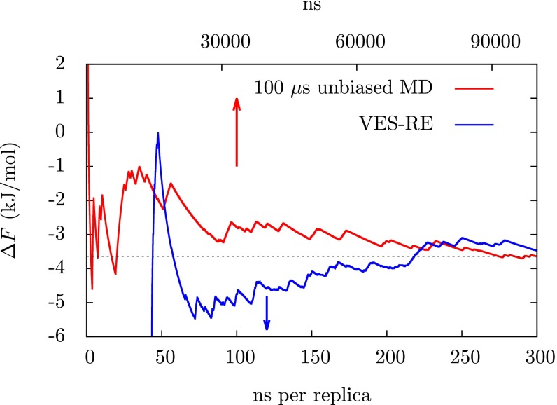
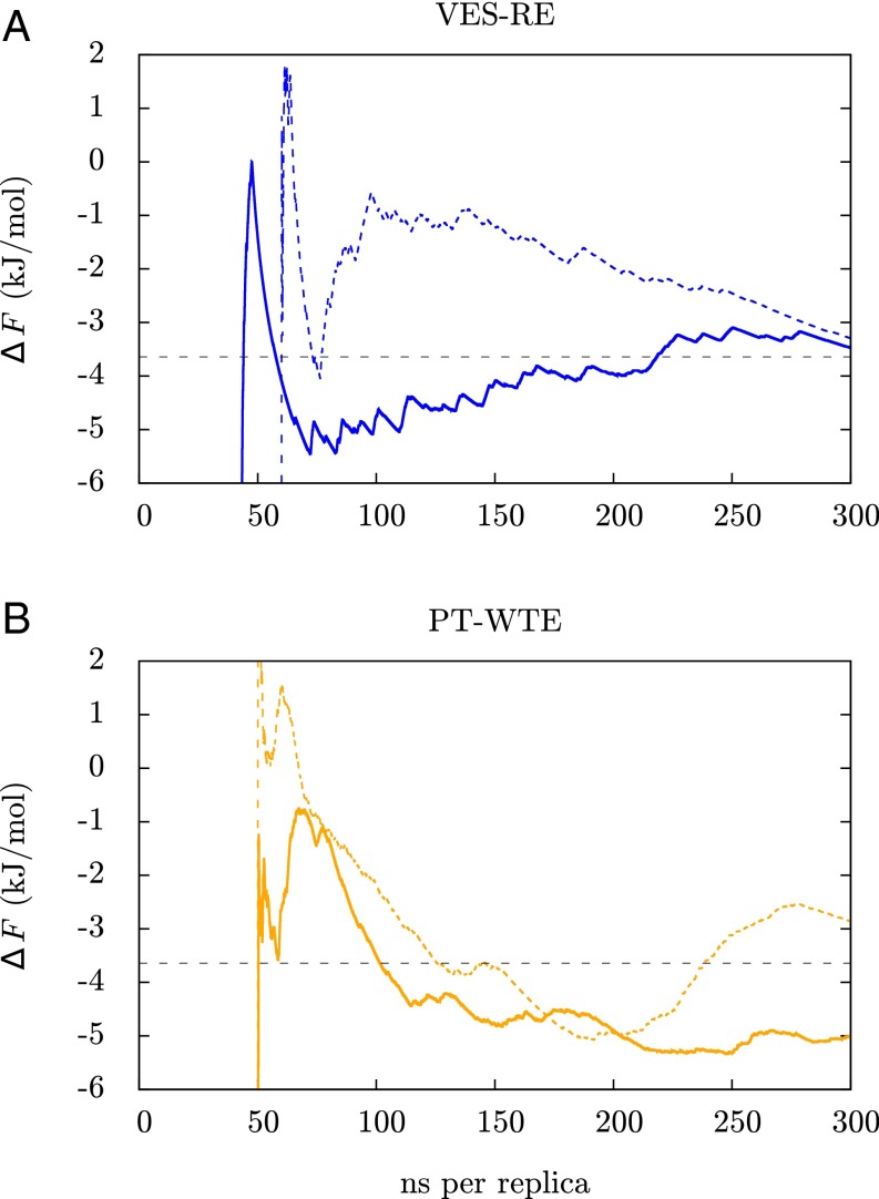
The details of the RE we use are described in Materials and Methods. We will refer to this approach as VES-RE. In Fig. 2 we show how an estimate of the folding free energy obtained from the lowest, unbiased replica converges over simulation time. The way we obtain this estimate is described in the Supporting Information. For comparison we also show the same quantity calculated from the 100-μs unbiased MD trajectory from ref. 1. Results from VES-RE are shown for a set of replicas which were initiated in the folded state. Within 300 ns per replica the folding free energy has converged almost exactly to the result obtained from the unbiased MD trajectory, with small fluctuations on the order of $\sim$0.5 kJ/mol. For the unbiased MD simulation it takes nearly the entire 100 μs to obtain a converged result. This is an order of magnitude improvement in efficiency and it is very likely that it could be improved further by, for example, using information from the biased replicas. One of the most important tests of convergence for a simulation that samples a complex transformation is how sensitive the results are to initial conditions. To rule out such a dependence on initial conditions we also did a calculation in which all replicas were initiated in an extended state and we find that the estimate of the folding free energy from this calculation agrees very well with the result in Fig. 2. These results are presented in Fig. 3A. For comparison with a standard method, we have also performed a parallel tempering simulation in the well-tempered ensemble (PT-WTE) (39, 40), which we describe in the Supporting Information. These results are shown in Fig. 3B, where it is clear that 300 ns per replica is not sufficient to obtain a converged estimate of the folding free energy from PT-WTE. In the Supporting Information we show that transitions between the folded and the unfolded state are extremely rare for continuous trajectories from PT-WTE, i.e., those that are reconstructed from jumps between the different replicas, which is crucial for efficient RE simulations.

Fig. 2.

Estimates of the folding free energy as a function of simulation time from VES-RE and unbiased MD. The quantity $\mathrm{\Delta }F$ is calculated according to Eq. S1 as described in the Supporting Information. The red line is from the 100-μs unbiased MD trajectory from ref. 1, the blue line is from VES-RE, and the horizontal black line is the converged value from the unbiased MD simulation for reference. The time scale for the unbiased MD simulation from ref. 1 is displayed on the top x axis and the time scale for VES-RE is displayed on the bottom x axis; arrows point to the appropriate axes. The first 50 ns of the VES-RE simulation was considered an equilibration period and was not used to estimate the folding free energy. To make an exact comparison of the computational resources used, one must consider that there were 12 replicas required for VES-RE.

Fig. 3.

Convergence of the estimate of the folding free energy from VES-RE (A) and PT-WTE (B). We show results from simulations in which all replicas were initiated in the folded state (solid lines) and simulations in which all replicas were initiated in the unfolded state (dashed lines). The horizontal black line indicates the converged result from 100-μs unbiased MD (1). Within 300 ns of simulation time per replica, both of the VES-RE calculations and the result from 100-μs unbiased MD agree with each other within 0.5 kJ/mol, indicating that we can accurately estimate the folding free energy this way regardless of initial conditions. The PT-WTE calculations clearly have not converged in this time scale.

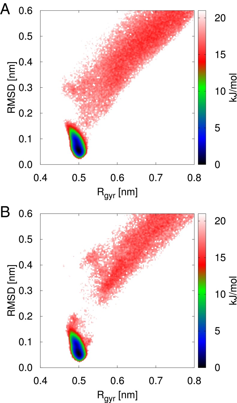
We can also measure free-energy surfaces of any order parameter we like from the unbiased replica in VES-RE. These are calculated by using a histogram to estimate the probability distribution of the order parameter ($n\left(\mathbf{s}\right)$), and then using the relationship $F\left(\mathbf{s}\right)=-\left(1/\beta \right)\log n\left(\mathbf{s}\right)$. In Fig. 4 we show the free-energy surface as a function of the Cα RMSD from the reference structure and the radius of gyration of the α-carbon atoms. For comparison we show the same free-energy surface estimated from the 100-μs unbiased MD trajectory. We find excellent agreement between the two methods. In particular, all of the regions below $\sim$15 kJ/mol are very well sampled. The small discrepancies in the transition state regions are due to difficulties that RE methods have in sampling the very low probability regions around barriers.

Fig. 4.

Comparison between free-energy surfaces as a function of the Cα RMSD from the reference structure and the radius of gyration of the α-carbon atoms obtained from 100-μs unbiased MD trajectory from ref. 1 (A) and VES-RE (B). The folded state minimum in these surfaces is set to zero and we only display features up to 20 kJ/mol.

Conclusions

We have presented results that illustrate some of the unique capabilities of the VES method introduced in ref. 14. We have shown that we can bias high-dimensional systems by choosing an appropriate, simplified representation of the bias and by making an intelligent choice of target distribution. This makes it possible to generate biasing potentials that efficiently and reversibly drive the system back and forth between the folded state and a disordered state of a small protein. This capability is extremely important for any study of the folding transition, and we have shown that it forms the basis for an efficient RE procedure that allows one to obtain statistics of the unbiased ensemble. Statistics generated in this way reproduce those obtained from 100-μs MD simulations on specialized hardware with extremely high accuracy at a fraction of the computational cost. The tradeoff for this dramatic reduction in computational resources is that we must make use of some information about the equilibrium structure in designing the target distribution, and that all dynamical information is lost in the RE procedure. Recent improvements in extracting rate constants from biased simulations (24, 41) may make it possible to overcome the latter limitation.

Foreseeable extensions of the methods we have described here have many exciting and interesting applications. In particular, the idea of using the target distribution to sample transitions between a localized state and a disordered state could be extremely useful for problems like ligand binding and unbinding. Accurately estimating the binding free energy of ligands is an extremely important and still very difficult calculation. We also imagine combining this method with tools like Rosetta which can predict protein structure based on the primary sequence (42). Another avenue we have not explored in this work is studying the high-dimensional free-energy surface itself. Accurate, high-dimensional free-energy surfaces could be an ideal way to construct coarse-grained models, and they could form the basis for novel studies of protein physics. The free-energy landscape of a protein must have several unique properties so that the protein does not get trapped in metastable states, and so that it can find the folded state in minimal time. Much of our current understanding of protein-folding free-energy landscapes is informed by studies of simplified, lattice-based models (43), and the approach we describe here might complement such studies.

Materials and Methods

MD Simulations.

All simulations of chignolin (sequence TYR-TYR-ASP-PRO-GLU-THR-GLY-THR-TRP-TYR) were conducted with GROMACS 4.6.5 (44) with a modified version of the PLUMED 2 plugin (45). The CHARMM22* force field (46) and the three-site transferrable intermolecular potential (TIP3P) water model (47) were used to make direct comparisons with ref. 1. ASP and GLU residues were simulated in their charged states, as were the N- and C-terminal amino acids. A timestep of 2 fs was used for all systems and constant temperature of 340 K (in agreement with ref. 1) was maintained by the velocity rescaling thermostat of Bussi et al. (48). All bonds involving H atoms were constrained with the linear constraint solver (LINCS) algorithm (49). Electrostatic interactions were calculated with the particle mesh Ewald scheme using a Fourier spacing of 0.12 nm and a real space cutoff of 0.95 nm (50). The same real space cutoff was also applied to van der Waals interactions. Initial configurations were generated by running a short 1-ns constant pressure (NPT) simulation with the protein in the folded state to allow the box size to equilibrate using the Parrinello–Rahman barostat (51). Subsequent runs were all conducted with fixed box size. The final cubic box had a side length of 4.044 nm and it had 2,122 water molecules, along with 2 sodium ions to neutralize the charge.

RE Procedure with VES Optimized Bias.

The RE procedure used is similar in spirit to Hamiltonian RE, solute tempering, and RE with CV tempering (17, 52, 53). In each replica the system is biased by the converged bias potential from the optimization run, scaled by a constant factor. The bias applied on replica i is $\left(1-\left(1/{\gamma }_i\right)\right)V\left(s\right)$, where ${\gamma }_i$ determines the strength of the bias applied. In the lowest replica, ${\gamma }_i=1$ and the system is unbiased. ${\gamma }_i$ then increases geometrically as one goes up the ladder of replicas. For the chignolin system studied here we used 12 replicas and the highest replica had $\gamma =18$. Exchange moves were attempted every 20 ps and accepted or rejected according to a Metropolis criterion. To satisfy detailed balance an exchange move must have an acceptance probability:

$$\text{acc}=\text{min}\left(1,e^{-\mathrm{\Delta }}\right),$$ [9]

where

$$\mathrm{\Delta }=\beta \left[V_i\left(s_j\right)+V_j\left(s_i\right)-V_i\left(s_i\right)+V_j\left(s_j\right)\right],$$ [10]

where $s_i$ is the value of the order parameters in ensemble i and $V_i$ is the bias used in ensemble i. In principle one could also use information extracted from the biased replicas to speed up the convergence of the free-energy surfaces shown in Fig. 4. One could also imagine optimizing the choices of ${\gamma }_i$ the way that Trebst et al. optimize the choice of temperatures for standard parallel tempering (54) but neither of these improvements was necessary for the present study.

Optimization of Biasing Potential

As mentioned in the main text, the optimization of the biasing potential proceeds by expanding the bias in a set of basis functions (Eq. 3), and treating the expansion coefficients as variational parameters. The gradient $\nabla \mathrm{\Omega }\left(\mathit{\alpha }\right)$ and Hessian $\mathbf{H}\left(\mathit{\alpha }\right)$ with respect to these parameters have a very simple form:

$$\frac{\partial \mathrm{\Omega }\left(\mathit{\alpha }\right)}{\partial {\alpha }_i}=-{\langle f_i\left(\mathbf{s}\right)\rangle }_{V\left(\mathbf{s};\mathbf{\alpha }\right)}+{\langle f_i\left(\mathbf{s}\right)\rangle }_{p\left(\mathbf{s}\right)},$$ [S1]

and

$$\frac{{\partial }^2\mathrm{\Omega }\left(\mathit{\alpha }\right)}{\partial {\alpha }_i\partial {\alpha }_j}=\beta \cdot \text{cov}{\left[f_i\left(\mathbf{s}\right),f_j\left(\mathbf{s}\right)\right]}_{V\left(\mathbf{s};\mathbf{\alpha }\right)}.$$ [S2]

The averages with subscript $V\left(\mathbf{s};\mathbf{\alpha }\right)$ are taken in the biased ensemble, which has probability distribution proportional to $e^{-\beta \left[F\left(\mathbf{s}\right)+V\left(\mathbf{s};\mathit{\alpha }\right)\right]}$, with parameters fixed at $\mathit{\alpha }$, and the averages with subscript $p\left(\mathbf{s}\right)$ are taken over the target distribution. The latter can often be computed analytically or numerically whereas the former must be estimated from sampling. At any given iteration it would take extremely long sampling times to accurately estimate these averages from the biased ensemble. We can drastically reduce the required sampling time if we use an appropriate stochastic optimization algorithm like the one described in ref. 29. In this algorithm we update the $\mathit{\alpha }$ parameters using the expression

$${\mathit{\alpha }}^{\left(n+1\right)}={\mathit{\alpha }}^{\left(n\right)}-\mu \left[\nabla \mathrm{\Omega }\left({\overline{\mathit{\alpha }}}^{\left(n\right)}\right)+\mathbf{H}\left({\overline{\mathit{\alpha }}}^{\left(n\right)}\right)\left[{\mathit{\alpha }}^{\left(n\right)}-{\overline{\mathit{\alpha }}}^{\left(n\right)}\right]\right],$$ [S3]

where we have introduced the averaged parameters ${\overline{\mathit{\alpha }}}^{\left(n\right)}$, which are defined by

$${\overline{\mathit{\alpha }}}^{\left(n\right)}={\left(n+1\right)}^{-1}{\displaystyle \sum _{l=0}^n{\mathit{\alpha }}^{\left(l\right)}}.$$ [S4]

The instantaneous parameters, ${\mathit{\alpha }}^n$, here play only an auxiliary role, as all sampling is conducted at ${\overline{\mathit{\alpha }}}^{\left(n\right)}$. The evaluation of the gradient and the Hessian will still be subject to stochastic error but the evolution of ${\overline{\mathit{\alpha }}}^{\left(n\right)}$ will be smooth due to the averaging procedure in Eq. S4 and one can afford a much shorter time averaging between successive iterations. A mathematical justification of this procedure can be found in ref. 29. This stochastic optimization approach has proven to be an effective choice to perform the minimization of $\mathrm{\Omega }\left[V\right]$, although other choices are certainly possible.

The optimization procedure described above requires a choice of basis set. With the dihedral angles as CVs, the natural choice is a Fourier basis. Each pairwise term was expanded as

$$V\left({\theta }_s,{\theta }_{s+1}\right)={\displaystyle \sum _{l,m}{\overline{\alpha }}_{l,m}\text{exp}\left(-i{k}_l{\theta }_s\right)\text{exp}\left(-i{k}_m{\theta }_{s+1}\right)}.$$ [S5]

We used 13 Fourier modes for each component for a total of 169 basis functions per pairwise term. The optimization parameter μ, which determines the step size in the iteration of Eq. S3, was chosen to be 0.001. Higher values of this parameter make the optimization less robust. Each iteration was 500 MD time steps, or 1 ps. The optimization was conducted with a multiple walkers scheme (55) in which six independent copies of the system are simulated simultaneously and statistics from each walker contribute to the averages in Eq. S1. It took about 200 ns to produce a converged bias potential. All of these parameters may be subject to refinement.

Convergence of Biasing Potential

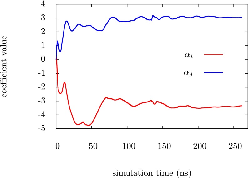
The simplest and most straightforward way to check for convergence of the bias potential (and thus minimization of the functional $\mathrm{\Omega }\left[V\right]$) is to monitor the expansion coefficients of the bias. Although there are over 3,000 expansion coefficients the majority of them are very small and largely irrelevant. We have selected the largest expansion coefficients from two of the pairwise biases for illustration purposes; these components have clearly converged after ∼200 ns and the same general behavior is observed for other components. An exact convergence of the bias is not critical in this work because we only collect statistics from the unbiased ensemble in the replica exchange scheme. We are mainly interested in the fact that the bias can drive the protein back and forth between the folded state and the unfolded state.

Folding of Chignolin with Different Values of $w_f$

As mentioned in the main text, $w_f=w_u=1/2$ is not necessarily the optimal choice for the weights in the target distribution and we have performed a few calculations with different values of these weights. In Fig. S2 we present the time series for the case where $w_f=0.85$ and we find that transitions between the folded state and the unfolded state are somewhat accelerated. For higher values of $w_f$ the system can have problems getting stuck in artificial minima and never find the folded state.

Fig. S1.

Evidence that the largest variational parameters converge over simulation time. ${\alpha }_i$ is the largest Fourier component of $V\left({\psi }_1,{\varphi }_2\right)$ and ${\alpha }_j$ is the largest Fourier component of $V\left({\varphi }_5,{\psi }_5\right)$.

Fig. S2.

Time series of the Cα RMSD from the reference structure for chignolin during the optimization process with $w_f$ = 0.85.

Components of Optimized Bias

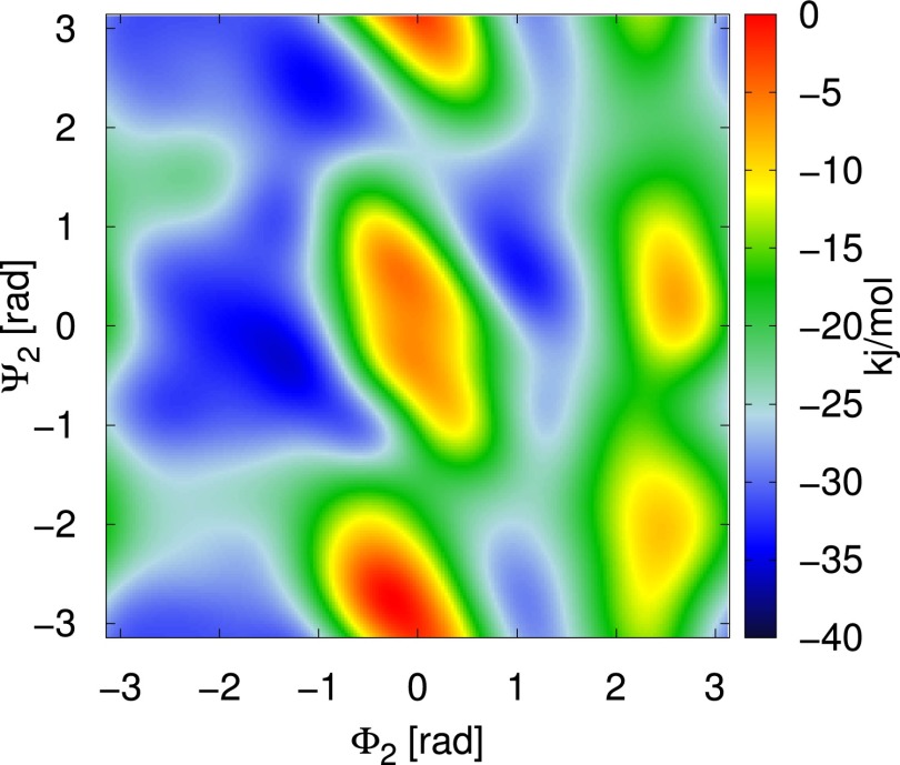
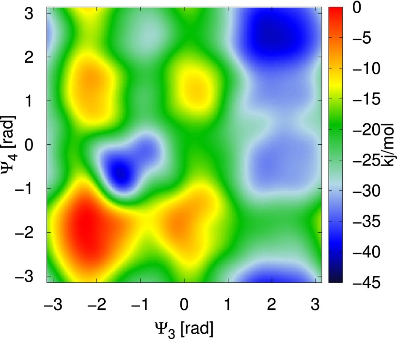
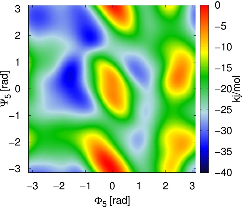
For reference we present a few of the pairwise terms that make up the optimized bias. We present the inverses of the biases because these are most closely related to the free-energy surface. It is important to recall that these surfaces do not have a direct interpretation as components of the free-energy surface because they do not include the $\left(1/\beta \right)\log p\left(\mathbf{s}\right)$ term, but they do give an impression of the local wells and barriers.

Estimate of the Folding Free Energy from the Unbiased Replica

The estimate of the folding free energy for chignolin was calculated as follows: every 100 ps the configuration of the protein in the unbiased replica was designated as either folded or unfolded based on RMSD and then the number of folded configurations, $n_{\text{fold}}$, and unfolded configurations, $n_{\text{unfold}}$, was calculated as a function of simulation time. The folding free energy is then calculated from

$$\mathrm{\Delta }F=-\frac{1}{\beta }\log \left(\frac{n_{\text{fold}}}{n_{\text{unfold}}}\right).$$ [S6]

The same approach was applied to estimate the folding free energy from the PT-WTE calculations, except instead of using the unbiased replica the lowest temperature replica was used.

PT-WTE

Reference data were generated from PT-WTE. This method uses the WTE to increase fluctuations of the potential energy (39), which allows one to greatly reduce the number of replicas required to span a given temperature range (40). The temperatures of the 12 replicas, which were distributed between 340 and 681 K, were chosen in an optimal way according to ref. 56. This temperature range is chosen to be similar to that used in previous studies (33), where the highest temperature seems to allow thorough exploration of the unfolded state. To construct the history-dependent bias, Gaussians were deposited with a width of 140 kJ/mol and an initial hill height of 1.2 kJ/mol every 0.6 ps. The bias factor γ, which controls how much the fluctuations of the potential energy are enhanced, was chosen to be 20. Exchange moves between replicas were attempted every 10 ps.

Slow Convergence in PT-WTE

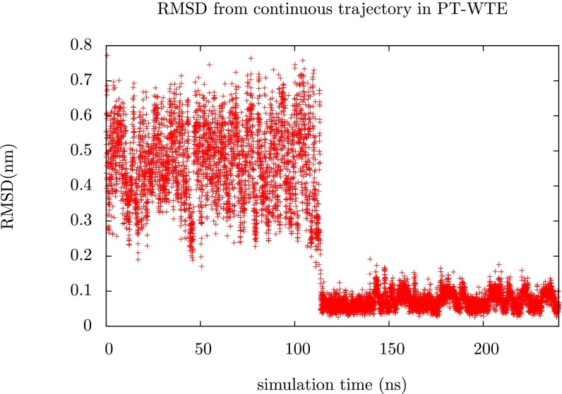
PT-WTE and standard PT simulations of proteins are very difficult to converge because transitions between the folded and the unfolded state are extremely rare in continuous trajectories. In Fig. S6 we show how the RMSD evolves over time for a single continuous trajectory (reconstructed from exchange moves) from the PT-WTE simulations described in the main text. We see that this trajectory has a single transition from unfolded to folded. Of the 12 continuous trajectories that comprised the PT-WTE run, 5 have no transitions between folded and unfolded, 4 have 1 transition, and 3 have 2 transitions for a total of 10 transitions. By contrast, transitions are much more common in the continuous trajectories from VES-RE. Of the 12 continuous trajectories from VES-RE, 9 have between 3 and 1 transitions, whereas the remaining 3 have 4, 5, and 6 transitions, amounting to 33 transitions in total.

Fig. S3.

Negative of the 2D bias that acts on the dihedral angles ${\varphi }_2$ and ${\psi }_2$.

Fig. S4.

Negative of the 2D bias that acts on the dihedral angles ${\psi }_3$ and ${\psi }_4$.

Fig. S5.

Negative of the 2D bias that acts on the dihedral angles ${\varphi }_5$ and ${\psi }_5$.

Fig. S6.

Cα RMSD for a continuous trajectory from the PT-WTE calculation described in the main text.

Reference Structures and CVs Used for Analysis

The reference angles used in the target distribution ($\overline{{\theta }_i}$) and the Cα RMSD CV are both based on a reference structure of the protein. This reference structure was generated from a short, unbiased MD simulation that started from the experimental crystal structure [Protein Data Bank ID code 5AWL (30)]. This reference structure is a better reflection of the actual folded state of the protein in the CHARMM22* force field than the crystal structure, but we have found that the results are not very sensitive to the exact reference structure used. In this section, we provide the exact values of the reference angles used in the target. These reference angles are listed in Table S1, and we list only those angles which are biased in the simulation.

Table S1.

Every dihedral angle which is biased in the simulations of chignolin, along with the reference angles (in radians) used to define the target distribution

Dihedral angle	Reference value, rad
${\psi }_1$	2.41
${\varphi }_2$	−2.52
${\psi }_2$	1.98
${\varphi }_3$	−1.58
${\psi }_3$	1.98
${\psi }_4$	−0.26
${\varphi }_5$	−0.89
${\psi }_5$	−1.15
${\varphi }_6$	−1.58
${\psi }_6$	−0.36
${\varphi }_7$	1.44
${\psi }_7$	0.078
${\varphi }_8$	−1.18
${\psi }_8$	1.86
${\varphi }_9$	−1.31
${\psi }_9$	2.35
${\varphi }_{10}$	−2.65

References

- 1.Lindorff-Larsen K, Piana S, Dror RO, Shaw DE. How fast-folding proteins fold. Science. 2011;334(6055):517–520. doi: 10.1126/science.1208351. [DOI] [PubMed] [Google Scholar]
- 2.Pan AC, Borhani DW, Dror RO, Shaw DE. Molecular determinants of drug-receptor binding kinetics. Drug Discov Today. 2013;18(13-14):667–673. doi: 10.1016/j.drudis.2013.02.007. [DOI] [PubMed] [Google Scholar]
- 3.Tiwary P, Limongelli V, Salvalaglio M, Parrinello M. Kinetics of protein-ligand unbinding: Predicting pathways, rates, and rate-limiting steps. Proc Natl Acad Sci USA. 2015;112(5):E386–E391. doi: 10.1073/pnas.1424461112. [DOI] [PMC free article] [PubMed] [Google Scholar]
- 4.Laio A, Parrinello M. Escaping free-energy minima. Proc Natl Acad Sci USA. 2002;99(20):12562–12566. doi: 10.1073/pnas.202427399. [DOI] [PMC free article] [PubMed] [Google Scholar]
- 5.Torrie G, Valleau J. Nonphysical sampling distributions in Monte Carlo free-energy estimation: Umbrella sampling. J Comput Phys. 1977;23(2):187–199. [Google Scholar]
- 6.Huber T, Torda AE, van Gunsteren WF. Local elevation: A method for improving the searching properties of molecular dynamics simulation. J Comput Aided Mol Des. 1994;8(6):695–708. doi: 10.1007/BF00124016. [DOI] [PubMed] [Google Scholar]
- 7.Darve E, Pohorille A. Calculating free energies using average force. J Chem Phys. 2001;115(20):9169–9183. [Google Scholar]
- 8.Hansmann UHE, Wille LT. Global optimization by energy landscape paving. Phys Rev Lett. 2002;88(6):068105. doi: 10.1103/PhysRevLett.88.068105. [DOI] [PubMed] [Google Scholar]
- 9.Wang F, Landau DP. Efficient, multiple-range random walk algorithm to calculate the density of states. Phys Rev Lett. 2001;86(10):2050–2053. doi: 10.1103/PhysRevLett.86.2050. [DOI] [PubMed] [Google Scholar]
- 10.Barducci A, Bussi G, Parrinello M. Well-tempered metadynamics: A smoothly converging and tunable free-energy method. Phys Rev Lett. 2008;100(2):020603. doi: 10.1103/PhysRevLett.100.020603. [DOI] [PubMed] [Google Scholar]
- 11.Maragakis P, van der Vaart A, Karplus M. Gaussian-mixture umbrella sampling. J Phys Chem B. 2009;113(14):4664–4673. doi: 10.1021/jp808381s. [DOI] [PMC free article] [PubMed] [Google Scholar]
- 12.Whitmer JK, et al. Sculpting bespoke mountains: Determining free energies with basis expansions. J Chem Phys. 2015;143(4):044101. doi: 10.1063/1.4927147. [DOI] [PubMed] [Google Scholar]
- 13.Bartels C, Karplus M. Multidimensional adaptive umbrella sampling: Applications to main chain and side chain peptide conformations. J Comput Chem. 1997;18(12):1450–1462. [Google Scholar]
- 14.Valsson O, Parrinello M. Variational approach to enhanced sampling and free energy calculations. Phys Rev Lett. 2014;113(9):090601. doi: 10.1103/PhysRevLett.113.090601. [DOI] [PubMed] [Google Scholar]
- 15.Piana S, Laio A. A bias-exchange approach to protein folding. J Phys Chem B. 2007;111(17):4553–4559. doi: 10.1021/jp067873l. [DOI] [PubMed] [Google Scholar]
- 16.Pfaendtner J, Bonomi M. Efficient sampling of high-dimensional free-energy landscapes with parallel bias metadynamics. J Chem Theory Comput. 2015;11(11):5062–5067. doi: 10.1021/acs.jctc.5b00846. [DOI] [PubMed] [Google Scholar]
- 17.Gil-Ley A, Bussi G. Enhanced conformational sampling using replica exchange with collective-variable tempering. J Chem Theory Comput. 2015;11(3):1077–1085. doi: 10.1021/ct5009087. [DOI] [PMC free article] [PubMed] [Google Scholar]
- 18.Kannan S, Zacharias M. Enhanced sampling of peptide and protein conformations using replica exchange simulations with a peptide backbone biasing-potential. Proteins. 2007;66(3):697–706. doi: 10.1002/prot.21258. [DOI] [PubMed] [Google Scholar]
- 19.Tribello GA, Ceriotti M, Parrinello M. A self-learning algorithm for biased molecular dynamics. Proc Natl Acad Sci USA. 2010;107(41):17509–17514. doi: 10.1073/pnas.1011511107. [DOI] [PMC free article] [PubMed] [Google Scholar]
- 20.Chen M, Yu TQ, Tuckerman ME. Locating landmarks on high-dimensional free energy surfaces. Proc Natl Acad Sci USA. 2015;112(11):3235–3240. doi: 10.1073/pnas.1418241112. [DOI] [PMC free article] [PubMed] [Google Scholar]
- 21.Abrams CF, Vanden-Eijnden E. Large-scale conformational sampling of proteins using temperature-accelerated molecular dynamics. Proc Natl Acad Sci USA. 2010;107(11):4961–4966. doi: 10.1073/pnas.0914540107. [DOI] [PMC free article] [PubMed] [Google Scholar]
- 22.Abrams C, Bussi G. Enhanced sampling in molecular dynamics using metadynamics, replica-exchange, and temperature-acceleration. Entropy (Basel) 2014;16(1):163–199. [Google Scholar]
- 23.Valsson O, Parrinello M. Well-tempered variational approach to enhanced sampling. J Chem Theory Comput. 2015;11(5):1996–2002. doi: 10.1021/acs.jctc.5b00076. [DOI] [PubMed] [Google Scholar]
- 24.McCarty J, Valsson O, Tiwary P, Parrinello M. Variationally optimized free-energy flooding for rate calculation. Phys Rev Lett. 2015;115(7):070601. doi: 10.1103/PhysRevLett.115.070601. [DOI] [PubMed] [Google Scholar]
- 25.de Boer PT, Kroese DP, Mannor S, Rubinstein RY. A tutorial on the cross-entropy method. Ann Oper Res. 2005;134(1):19–67. [Google Scholar]
- 26.Chaimovich A, Shell MS. Coarse-graining errors and numerical optimization using a relative entropy framework. J Chem Phys. 2011;134(9):094112. doi: 10.1063/1.3557038. [DOI] [PubMed] [Google Scholar]
- 27.Bilionis I, Koutsourelakis PS. Free energy computations by minimization of Kullback-Leibler divergence: An efficient adaptive biasing potential method for sparse representations. J Comput Phys. 2012;231(9):3849–3870. [Google Scholar]
- 28.Zhang W, Wang H, Hartmann C, Weber M, Schutte C. Applications of the cross-entropy method to importance sampling and the optimal control of diffusions. SIAM J Sci Comput. 2014;36(6):2654–2672. [Google Scholar]
- 29.Bach F, Moulines E. 2013. Non-strongly-convex smooth stochastic approximation with convergence rate O (1/n). Advances in Neural Information Processing Systems 26 (NIPS 2013), eds Burges CJC, Bottou L, Welling M, Ghahramani Z, Weinberger KQ (Curran Associates, Inc., Red Hook, NY), pp 773–781.
- 30.Honda S, et al. Crystal structure of a ten-amino acid protein. J Am Chem Soc. 2008;130(46):15327–15331. doi: 10.1021/ja8030533. [DOI] [PubMed] [Google Scholar]
- 31.Miao Y, Feixas F, Eun C, McCammon JA. Accelerated molecular dynamics simulations of protein folding. J Comput Chem. 2015;36(20):1536–1549. doi: 10.1002/jcc.23964. [DOI] [PMC free article] [PubMed] [Google Scholar]
- 32.Zhang T, Nguyen PH, Nasica-Labouze J, Mu Y, Derreumaux P. Folding atomistic proteins in explicit solvent using simulated tempering. J Phys Chem B. 2015;119(23):6941–6951. doi: 10.1021/acs.jpcb.5b03381. [DOI] [PubMed] [Google Scholar]
- 33.Kührová P, De Simone A, Otyepka M, Best RB. Force-field dependence of chignolin folding and misfolding: Comparison with experiment and redesign. Biophys J. 2012;102(8):1897–1906. doi: 10.1016/j.bpj.2012.03.024. [DOI] [PMC free article] [PubMed] [Google Scholar]
- 34.Szabo A, Ostlund N. Modern Quantum Chemistry: Introduction to Advanced Electronic Structure Theory. Macmillan; New York: 1982. [Google Scholar]
- 35.Gerber S, Horenko I. On inference of causality for discrete state models in a multiscale context. Proc Natl Acad Sci USA. 2014;111(41):14651–14656. doi: 10.1073/pnas.1410404111. [DOI] [PMC free article] [PubMed] [Google Scholar]
- 36.Hansmann UHE. Parallel tempering algorithm for conformational studies of biological molecules. Chem Phys Lett. 1997;281:140–150. [Google Scholar]
- 37.Sugita Y, Okamoto Y. Replica exchange molecular dynamics method for protein folding simulation. Chem Phys Lett. 1999;314:141–151. [Google Scholar]
- 38.Rosta E, Hummer G. Error and efficiency of replica exchange molecular dynamics simulations. J Chem Phys. 2009;131(16):165102. doi: 10.1063/1.3249608. [DOI] [PMC free article] [PubMed] [Google Scholar]
- 39.Bonomi M, Parrinello M. Enhanced sampling in the well-tempered ensemble. Phys Rev Lett. 2010;104(19):190601. doi: 10.1103/PhysRevLett.104.190601. [DOI] [PubMed] [Google Scholar]
- 40.Deighan M, Bonomi M, Pfaendtner J. Efficient simulation of explicitly solvated proteins in the well-tempered ensemble. J Chem Theory Comput. 2012;8(7):2189–2192. doi: 10.1021/ct300297t. [DOI] [PubMed] [Google Scholar]
- 41.Tiwary P, Parrinello M. From metadynamics to dynamics. Phys Rev Lett. 2013;111(23):230602. doi: 10.1103/PhysRevLett.111.230602. [DOI] [PubMed] [Google Scholar]
- 42.Rohl CA, Strauss CEM, Misura KMS, Baker D. Protein structure prediction using Rosetta. Methods Enzymol. 2004;383:66–93. doi: 10.1016/S0076-6879(04)83004-0. [DOI] [PubMed] [Google Scholar]
- 43.Dinner AR, Šali A, Smith LJ, Dobson CM, Karplus M. Understanding protein folding via free-energy surfaces from theory and experiment. Trends Biochem Sci. 2000;25(7):331–339. doi: 10.1016/s0968-0004(00)01610-8. [DOI] [PubMed] [Google Scholar]
- 44.Hess B, Kutzner C, van der Spoel D, Lindahl E. GRGMACS 4: Algorithms for highly efficient, load-balanced, and scalable molecular simulation. J Chem Theory Comput. 2008;4(3):435–447. doi: 10.1021/ct700301q. [DOI] [PubMed] [Google Scholar]
- 45.Tribello GA, Bonomi M, Branduardi D, Camilloni C, Bussi G. PLUMED 2: New feathers for an old bird. Comput Phys Commun. 2014;185(2):604–613. [Google Scholar]
- 46.Piana S, Lindorff-Larsen K, Shaw DE. How robust are protein folding simulations with respect to force field parameterization? Biophys J. 2011;100(9):L47–L49. doi: 10.1016/j.bpj.2011.03.051. [DOI] [PMC free article] [PubMed] [Google Scholar]
- 47.Jorgensen WL, Chandrasekhar J, Madura JD, Impey RW, Klein ML. Comparison of simple potential functions for simulating liquid water. J Chem Phys. 1983;79(2):926. [Google Scholar]
- 48.Bussi G, Donadio D, Parrinello M. Canonical sampling through velocity rescaling. J Chem Phys. 2007;126(1):014101. doi: 10.1063/1.2408420. [DOI] [PubMed] [Google Scholar]
- 49.Hess B, Bekker H, Berendsen HJC, Fraaije JGEM. LINCS: A linear constraint solver for molecular simulations. J Comput Chem. 1997;18(12):1463–1472. [Google Scholar]
- 50.Essmann U, et al. A smooth particle mesh Ewald method. J Chem Phys. 1995;103:8577–8593. [Google Scholar]
- 51.Parrinello M. Polymorphic transitions in single crystals: A new molecular dynamics method. J Appl Phys. 1981;52(12):7182. [Google Scholar]
- 52.Liu P, Kim B, Friesner RA, Berne BJ. Replica exchange with solute tempering: A method for sampling biological systems in explicit water. Proc Natl Acad Sci USA. 2005;102(39):13749–13754. doi: 10.1073/pnas.0506346102. [DOI] [PMC free article] [PubMed] [Google Scholar]
- 53.Sugita Y, Okamoto Y. Replica-exchange multicanonical algorithm and multicanonical replica-exchange method for simulating systems with rough energy landscape. Chem Phys Lett. 2000;329(October):261–270. [Google Scholar]
- 54.Trebst S, Troyer M, Hansmann UHE. Optimized parallel tempering simulations of proteins. J Chem Phys. 2006;124(17):174903. doi: 10.1063/1.2186639. [DOI] [PubMed] [Google Scholar]
- 55.Raiteri P, Laio A, Gervasio FL, Micheletti C, Parrinello M. Efficient reconstruction of complex free energy landscapes by multiple walkers metadynamics. J Phys Chem B. 2006;110(8):3533–3539. doi: 10.1021/jp054359r. [DOI] [PubMed] [Google Scholar]
- 56.Prakash MK, Barducci A, Parrinello M. Replica temperatures for uniform exchange and efficient roundtrip times in explicit solvent parallel tempering simulations. J Chem Theory Comput. 2011;7(7):2025–2027. doi: 10.1021/ct200208h. [DOI] [PubMed] [Google Scholar]