

Abstract
There is a strong emphasis on developing novel neuroscience technologies, in particular on recording from more neurons. There has thus been increasing discussion about how to analyze the resulting big datasets. What has received less attention is that over the last 30 years, papers in neuroscience have progressively integrated more approaches, such as electrophysiology, anatomy, and genetics. As such, there has been little discussion on how to combine and analyze this multimodal data. Here, we describe the growth of multimodal approaches, and discuss the needed analysis advancements to make sense of this data.
Keywords: data integration, technology integration, large-scale data analysis, multimodal, neural data analysis
Evolution of Neuroscience Technologies and Questions
The development of neuroscience technology has been rapidly advancing (Stevenson and Kording, 2011; Insel et al., 2013; Kandel et al., 2013; Marblestone et al., 2013) across many approaches, including those that investigate neural activity (Kording, 2011; Prevedel et al., 2014; Schwarz et al., 2014; Van Horn and Toga, 2014; Vladimirov et al., 2014; Hamel et al., 2015; Lemon et al., 2015), neuroanatomy (Zador et al., 2012; Helmstaedter, 2013; Van Essen, 2013; Oh et al., 2014; Glaser et al., 2015), and gene expression and genetics (Cahoy et al., 2008; Stein et al., 2012; Lee et al., 2014; Medland et al., 2014). Advancing technologies allow us to answer more complex questions. For instance, with single electrodes, researchers could only ask about how individual neurons respond to stimuli and relate to behavior (Hubel and Wiesel, 1959; O’Keefe and Dostrovsky, 1971; Georgopoulos et al., 1982). With the invention of electrode arrays (Maynard et al., 1997; Schwarz et al., 2014; Siegel et al., 2015) and large-scale optical recording techniques (Prevedel et al., 2014; Vladimirov et al., 2014; Hamel et al., 2015), many now ask how neurons interact with each other (Cohen and Kohn, 2011; Stevenson and Kording, 2011; Cunningham and Yu, 2014). Data analysis techniques have been extended to make sense of this growing neural data (e.g., Pfau et al., 2013; Cunningham and Yu, 2014; Freeman et al., 2014; Gao and Ganguli, 2015), which has led to many important insights about the brain.
Along with developing new technologies and increasing the scalability of existing technologies, another way to answer more complex questions is to combine multiple approaches (e.g., using electrophysiology and neuroanatomy together). The brain is a complex system whose function depends on the interplay between countless structures and actions, all spanning different spatial and temporal scales. Combining multiple approaches is critical for understanding how different aspects of the brain relate to each other, e.g., how the morphology of a neuron influences its activity. Moreover, combining multiple approaches is critical for understanding how the brain operates at multiple scales, e.g., how the spikes of individual neurons are related to waves of activity spread across the brain. Data analysis techniques to make sense of this “multimodal” data will be very important going forward.
Growth of Multimodal Approaches
Multimodal approaches have been used for many years. As a classic example, Hubel and Wiesel (1962) used electrophysiology and anatomy to determine how the functional properties of cells were different across different layers of visual cortex. As a more recent example, researchers have simultaneously used gene expression techniques and tracing (anatomy) techniques to determine what cell types are connected to each other (Sorensen et al., 2015). Similarly, the Allen Brain Institute has been developing an atlas with integrated connectivity, gene expression, and neuroanatomical information (Sunkin et al., 2013). Such approaches allow us to understand how different modalities relate to each other, and how they together lead to brain function.
Have the amount of studies that combine technologies from multiple experimental modalities (Bock et al., 2011; Hofer et al., 2011; Annese, 2012; Sui et al., 2012; Sunkin et al., 2013; Marblestone et al., 2014; Uludağ and Roebroeck, 2014; Markram et al., 2015; Sorensen et al., 2015) been increasing? We looked in the PubMed database for the number of neuroscience articles that had anatomy, genetics, and/or electrophysiology (one common method of collecting activity) as a subject matter. Over time, the probability of two modalities co-occurring in the same paper increased, for each combination of the three modalities (Figure 1). Interestingly, this increase has occurred at different rates for different combinations of modalities (Figure 1); over the last 30 years, the relative co-occurrence of electrophysiology and anatomy has doubled, and the relative co-occurrences of electrophysiology and genetics, and anatomy and genetics have quadrupled. The integration of approaches is clearly accelerating.
Figure 1.
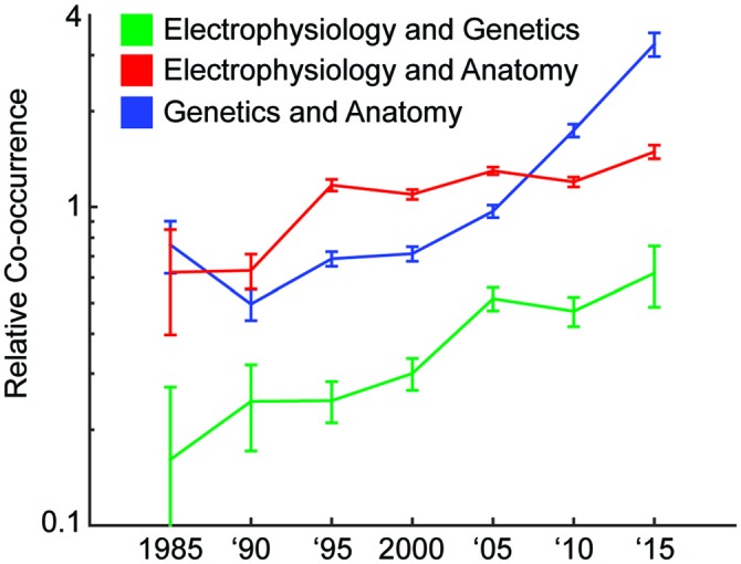
Increase of multimodal papers over time. We track how often different modalities of technology are used together over 5 year intervals. We do this by searching the PubMed database for papers with subjects representing the modalities. A relative co-occurrence (y-axis; plotted on a log-scale) of one means that occurrence of the two modalities in a paper is independent. A value greater than one means they are more likely to appear together, and a value less than one means they are more likely to appear apart.1
Gathering Multimodal Data to Understand Neural Activity
For the remainder of the paper, we focus on how multimodal approaches can help us understand neural activity, at the level of neurons (electrophysiology or calcium imaging, as opposed to neuroimaging). Prior to discussing how to analyze this data, it’s important to elaborate upon how this multimodal data can be acquired.
First of all, in many cases, we can gather information about additional modalities with standard activity (electrophysiology or calcium imaging) experiments. Trivially, activity recordings come with approximate neuroanatomy information. That is, we generally know what area of the brain is being recorded from. Additionally, we can get approximate information about cell type (inhibitory vs. excitatory) from electrophysiological waveforms (Mitchell et al., 2007). We can even get approximate estimates of structural connectivity using neural activity (Keshri et al., 2013; Fletcher and Rangan, 2014; Veeriah et al., 2015). Thus, truly multimodal experiments may not always be necessary to gather some forms of multimodal data.
Next, information about multiple modalities can be acquired via more complex experiments. For example, researchers have used calcium imaging followed by electron microscopy in order to determine the relation between neuroanatomy (e.g., connectivity) and neural activity (Bock et al., 2011). As another example, researchers have utilized modern genetic techniques to define cell types via gene expression, and then determine how neural activity differs between those cell types (e.g., Pinto and Dan, 2015). These experiments directly provide rich data from multiple modalities, and are critical for providing a ground truth about how modalities interact.
Lastly, it may be possible to combine information from multiple experiments from different subjects. While we generally cannot match specific neurons across subjects2, we can utilize statistical information from previous experiments. For example, we can use information about the likelihood of neurons being connected as a prior in a model that aims to explain neural activity (Rigat et al., 2006; Mishchenko et al., 2011). Additionally, previous information about the relationship between activity and another modality can be used. For example, suppose that cell types can be determined by looking at neural activity in response to varying stimuli (Farrow and Masland, 2011). Future experiments could first determine the cell type based on this previous knowledge, and then see how cell type relates to activity under novel experimental conditions. Utilizing data or knowledge from previous experiments can lead to important multimodal findings.
Analyzing Multimodal Data
Neural recording is scaling up, and multimodal approaches are increasing. There has been much discussion about how to analyze and build models from large neural activity datasets (Eliasmith and Trujillo, 2014; Gao and Ganguli, 2015; O’Leary et al., 2015). However, there has been little discussion about how additional modalities should be utilized for analyzing and modeling neural activity. These analyses will be crucial for determining how the interplay between different modalities leads to neural function.
One way to analyze this multimodal data is simply to use current analysis methods, and gain additional knowledge by labeling the results based on information about another modality. For example, we generally model the activity of a single neuron based on external factors (e.g., movement or stimuli) and the activity of other neurons (Stevenson et al., 2012; Fernandes et al., 2014; Park et al., 2014). With knowledge from another modality (e.g., cell type), we could first use this same approach. Then, we could look at the results in terms of the cell type to answer questions such as: Do the different cell types respond differently to external factors, and are neurons of certain cell types more likely to be functionally connected? Thus, when modeling the activity of single neurons, standard analysis approaches may be sufficient to answer some questions.
Similarly, it is possible to use current analysis methods to analyze multimodal data from large populations of neurons. When analyzing large populations of neurons, researchers often use dimensionality reduction techniques to better understand how neural activity of a population changes over time in relation to external factors (Mante et al., 2013; Shenoy et al., 2013; Cunningham and Yu, 2014). With information about additional modalities, we could separately use dimensionality reduction techniques on separate populations of neurons (e.g., those of different cell type; Armañanzas and Ascoli, 2015) to see how they differ. Related to dimensionality reduction techniques, researchers use latent variable models to model shared, but unobservable, variance between neurons (Sahani, 1999; Kulkarni and Paninski, 2007). These models could be better understood with knowledge about other modalities. For example, we could understand whether the shared variability is due to neurons sharing the same morphology, having similar gene expression, sharing synaptic inputs, or sharing neuromodulatory inputs. In general, by simply looking at differences between separate categories of neurons, many of our current analysis techniques can help us understand multimodal data.
Another method for utilizing multimodal data would be to analyze the neural activity as a function of other modalities. In the case of modeling the activity of individual neurons, another modality could act as a covariate in a predictive model. For example, a regression model of spikes could include local field potentials or fMRI as covariates. This would yield insight into how activity at a larger spatial and temporal scale influences local activity, i.e., how more global phenomena affect local, precise activity. As another example, suppose we aim to understand how gene expression is related to neurons’ response properties. First, the response properties (e.g., whether it has phasic or tonic responses to stimuli) could be quantified, and then the expression of many genes could be used as covariates to predict these responses. Predictive models can help us understand how other modalities influence activity of individual neurons.
Similarly, the activity of large populations of neurons can be modeled as a function of other modalities. To do this, the additional modalities can be utilized as constraints in latent variable or dimensionality reduction models. For instance, latent variable models could be enhanced by constraining the latent variables to be consistent with observations from other experimental modalities. That is, only neurons of a specific classification would share latent inputs. Another possibility would be to constrain dimensionality reduction techniques so that different classes of neurons would occupy different dimensions. This approach could be similar to targeted dimensionality reduction (Mante et al., 2013), which uses task-relevant variables as the different dimensions. Essentially, we would want to de-mix the activity into activity caused by each class of neurons. In general, constraints would allow more directly interpreting the outputs of these analysis techniques, to understand how these modalities predict activity.
Lastly, it could be especially beneficial to develop analysis methods that are specifically designed for analyzing multimodal data. Semedo et al. (2014) developed a latent variable model to look at the interaction between separate populations of neurons. While they used their method to investigate interactions between neurons from different brain areas, the technique could be used to look at interactions between any different classifications of neurons (differing morphology, gene expression, etc.). The authors make the important point that an alternative approach would be to first reduce the dimensionality of each population of neurons, and then look at their interaction. However, the separate dimensionality reduction could remove important aspects of the interaction between populations. Thus, their specific method for analyzing both populations simultaneously was important.
In the previous discussion, we have assumed that adding an additional modality would always be beneficial for modeling the neural activity. However, this may not always be the case; there may be explaining away across modalities. For example, if we have a lot of electrophysiological data, then connectomics data may become irrelevant, because the physiology already gives away a lot of connectivity information (Keshri et al., 2013; Fletcher and Rangan, 2014; Veeriah et al., 2015). Similarly, having both connectivity and cell type information may not be very beneficial, because connectivity information can predict cell types (Jonas and Kording, 2015). As such, there are a wide range of scenarios where recording from multiple modalities may not be overly useful. Further multimodal measurements are needed to determine how complementary vs. redundant different data sources are, as we move towards truly large datasets.
In an era when both the amount and the diversity of data is increasing, it’s critical to develop techniques that can help us make sense of this large-scale and multimodal data.
Author Contributions
JIG and KPK wrote the manuscript. JIG conducted the analyses.
Funding
We want to thank the NIH for funding (MH103910, NS074044, EY021579, EY025532).
Conflict of Interest Statement
The authors declare that the research was conducted in the absence of any commercial or financial relationships that could be construed as a potential conflict of interest. The reviewer, PL, and handling Editor declared their shared affiliation, and the handling Editor states that the process nevertheless met the standards of a fair and objective review.
Acknowledgments
We thank Ted Cybulski and Pat Lawlor for helpful comments.
Footnotes
1More details on how we generated Figure 1 are as follows. We tracked how often different modalities of technology were used together over 5 year intervals. We did this by searching the PubMed database for papers with subjects (“MeSH Terms” in the database) representing the modalities. Note that we searched for the terms “genetics” and “gene” for the genetics modality. We find the probability that, out of the neuroscience articles (those appearing when searching for “neuron”, “neural”, or “brain”), the subject matter contains one or two of the modalities. Let P(M1) be the probability of M1 being a subject of a paper, and P(M1, M2) be the probability of both M1 and M2 being subjects of a paper. The relative co-occurrence (y-axis) is P(M1, M2)/(P(M1) × P(M2)).
2Working on a larger scale than individual neurons (or in the case of c. elegans), matching information across subjects is more feasible. For example, to match connectomes, graph matching approaches are being used (Vogelstein et al., 2015). Others have matched information about diseases in humans and animal models using ontologies (Washington et al., 2009; Maynard et al., 2013).
References
- Annese J. (2012). The importance of combining MRI and large-scale digital histology in neuroimaging studies of brain connectivity and disease. Front. Neuroinform. 6:13 10.3389/fninf.2012.00013 [DOI] [PMC free article] [PubMed] [Google Scholar]
- Armañanzas R., Ascoli G. A. (2015). Towards the automatic classification of neurons. Trends Neurosci. 38, 307–318. 10.1016/j.tins.2015.02.004 [DOI] [PMC free article] [PubMed] [Google Scholar]
- Bock D. D., Lee W.-C. A., Kerlin A. M., Andermann M. L., Hood G., Wetzel A. W., et al. (2011). Network anatomy and in vivo physiology of visual cortical neurons. Nature 471, 177–182. 10.1038/nature09802 [DOI] [PMC free article] [PubMed] [Google Scholar]
- Cahoy J. D., Emery B., Kaushal A., Foo L. C., Zamanian J. L., Christopherson K. S., et al. (2008). A transcriptome database for astrocytes, neurons and oligodendrocytes: a new resource for understanding brain development and function. J. Neurosci. 28, 264–278. 10.1523/JNEUROSCI.4178-07.2008 [DOI] [PMC free article] [PubMed] [Google Scholar]
- Cohen M. R., Kohn A. (2011). Measuring and interpreting neuronal correlations. Nat. Neurosci. 14, 811–819. 10.1038/nn.2842 [DOI] [PMC free article] [PubMed] [Google Scholar]
- Cunningham J. P., Yu B. M. (2014). Dimensionality reduction for large-scale neural recordings. Nat. Neurosci. 17, 1500–1509. 10.1038/nn.3776 [DOI] [PMC free article] [PubMed] [Google Scholar]
- Eliasmith C., Trujillo O. (2014). The use and abuse of large-scale brain models. Curr. Opin. Neurobiol. 25, 1–6. 10.1016/j.conb.2013.09.009 [DOI] [PubMed] [Google Scholar]
- Farrow K., Masland R. H. (2011). Physiological clustering of visual channels in the mouse retina. J. Neurophysiol. 105, 1516–1530. 10.1152/jn.00331.2010 [DOI] [PMC free article] [PubMed] [Google Scholar]
- Fernandes H. L., Stevenson I. H., Phillips A. N., Segraves M. A., Kording K. P. (2014). Saliency and saccade encoding in the frontal eye field during natural scene search. Cereb. Cortex 24, 3232–3245. 10.1093/cercor/bht179 [DOI] [PMC free article] [PubMed] [Google Scholar]
- Fletcher A. K., Rangan S. (2014). “Scalable inference for neuronal connectivity from calcium imaging,” in Advances in Neural Information Processing Systems (NIPS), 2843–2851. [Google Scholar]
- Freeman J., Vladimirov N., Kawashima T., Mu Y., Sofroniew N. J., Bennett D. V., et al. (2014). Mapping brain activity at scale with cluster computing. Nat. Methods 11, 941–950. 10.1038/nmeth.3041 [DOI] [PubMed] [Google Scholar]
- Gao P., Ganguli S. (2015). On simplicity and complexity in the brave new world of large-scale neuroscience. Curr. Opin. Neurobiol. 32, 148–155. 10.1016/j.conb.2015.04.003 [DOI] [PubMed] [Google Scholar]
- Georgopoulos A. P., Kalaska J. F., Caminiti R., Massey J. T. (1982). On the relations between the direction of two-dimensional arm movements and cell discharge in primate motor cortex. J. Neurosci. 2, 1527–1537. [DOI] [PMC free article] [PubMed] [Google Scholar]
- Glaser J. I., Zamft B. M., Church G. M., Kording K. P. (2015). Puzzle imaging: using large-scale dimensionality reduction algorithms for localization. PLoS One 10:e0131593. 10.1371/journal.pone.0131593 [DOI] [PMC free article] [PubMed] [Google Scholar]
- Hamel E. J., Grewe B. F., Parker J. G., Schnitzer M. J. (2015). Cellular level brain imaging in behaving mammals: an engineering approach. Neuron 86, 140–159. 10.1016/j.neuron.2015.03.055 [DOI] [PMC free article] [PubMed] [Google Scholar]
- Helmstaedter M. (2013). Cellular-resolution connectomics: challenges of dense neural circuit reconstruction. Nat. Methods 10, 501–507. 10.1038/nmeth.2476 [DOI] [PubMed] [Google Scholar]
- Hofer S. B., Ko H., Pichler B., Vogelstein J., Ros H., Zeng H., et al. (2011). Differential connectivity and response dynamics of excitatory and inhibitory neurons in visual cortex. Nat. Neurosci. 14, 1045–1052. 10.1038/nn.2876 [DOI] [PMC free article] [PubMed] [Google Scholar]
- Hubel D. H., Wiesel T. N. (1959). Receptive fields of single neurones in the cat’s striate cortex. J. Physiol. 148, 574–591. 10.1113/jphysiol.1959.sp006308 [DOI] [PMC free article] [PubMed] [Google Scholar]
- Hubel D. H., Wiesel T. N. (1962). Receptive fields, binocular interaction and functional architecture in the cat’s visual cortex. J. Physiol. 160, 106–154. 10.1113/jphysiol.1962.sp006837 [DOI] [PMC free article] [PubMed] [Google Scholar]
- Insel T. R., Landis S. C., Collins F. S. (2013). The NIH brain initiative. Science 340, 687–688. 10.1038/nature.2013.13745 [DOI] [PMC free article] [PubMed] [Google Scholar]
- Jonas E., Kording K. (2015). Automatic discovery of cell types and microcircuitry from neural connectomics. eLife 4:e04250. 10.7554/elife.04250 [DOI] [PMC free article] [PubMed] [Google Scholar]
- Kandel E. R., Markram H., Matthews P. M., Yuste R., Koch C. (2013). Neuroscience thinks big (and collaboratively). Nat. Rev. Neurosci. 14, 659–664. 10.1038/nrn3578 [DOI] [PubMed] [Google Scholar]
- Keshri S., Pnevmatikakis E., Pakman A., Shababo B., Paninski L. (2013). A shotgun sampling solution for the common input problem in neural connectivity inference. arXiv preprint arXiv:1309.3724 [Google Scholar]
- Kording K. P. (2011). Of toasters and molecular ticker tapes. PLoS Comput. Biol. 7:e1002291. 10.1371/journal.pcbi.1002291 [DOI] [PMC free article] [PubMed] [Google Scholar]
- Kulkarni J. E., Paninski L. (2007). Common-input models for multiple neural spike-train data. Network 18, 375–407. 10.1080/09548980701625173 [DOI] [PubMed] [Google Scholar]
- Lee J. H., Daugharthy E. R., Scheiman J., Kalhor R., Yang J. L., Ferrante T. C., et al. (2014). Highly multiplexed subcellular RNA sequencing in situ. Science 343, 1360–1363. 10.1126/science.1250212 [DOI] [PMC free article] [PubMed] [Google Scholar]
- Lemon W. C., Pulver S. R., Höckendorf B., McDole K., Branson K., Freeman J., et al. (2015). Whole-central nervous system functional imaging in larval Drosophila. Nat. Commun. 6:7924. 10.1038/ncomms8924 [DOI] [PMC free article] [PubMed] [Google Scholar]
- Mante V., Sussillo D., Shenoy K. V., Newsome W. T. (2013). Context-dependent computation by recurrent dynamics in prefrontal cortex. Nature 503, 78–84. 10.1038/nature12742 [DOI] [PMC free article] [PubMed] [Google Scholar]
- Marblestone A. H., Daugharthy E. R., Kalhor R., Peikon I. D., Kebschull J. M., Shipman S. L., et al. (2014). Rosetta brains: a strategy for molecularly-annotated connectomics. arXiv preprint arXiv:1404.5103 [Google Scholar]
- Marblestone A. H., Zamft B. M., Maguire Y. G., Shapiro M. G., Cybulski T. R., Glaser J. I., et al. (2013). Physical principles for scalable neural recording. Front. Comput. Neurosci. 7:137. 10.3389/fncom.2013.00137 [DOI] [PMC free article] [PubMed] [Google Scholar]
- Markram H., Muller E., Ramaswamy S., Reimann M. W., Abdellah M., Sanchez C. A., et al. (2015). Reconstruction and simulation of neocortical microcircuitry. Cell 163, 456–492. 10.1016/j.cell.2015.09.029 [DOI] [PubMed] [Google Scholar]
- Maynard S. M., Mungall C. J., Lewis S. E., Imam F. T., Martone M. E. (2013). A knowledge based approach to matching human neurodegenerative disease and animal models. Front. Neuroinform. 7:7. 10.3389/fninf.2013.00007 [DOI] [PMC free article] [PubMed] [Google Scholar]
- Maynard E. M., Nordhausen C. T., Normann R. A. (1997). The Utah intracortical electrode array: a recording structure for potential brain-computer interfaces. Electroencephalogr. Clin. Neurophysiol. 102, 228–239. 10.1016/S0013-4694(96)95176-0 [DOI] [PubMed] [Google Scholar]
- Medland S. E., Jahanshad N., Neale B. M., Thompson P. M. (2014). Whole-genome analyses of whole-brain data: working within an expanded search space. Nat. Neurosci. 17, 791–800. 10.1038/nn.3718 [DOI] [PMC free article] [PubMed] [Google Scholar]
- Mishchenko Y., Vogelstein J. T., Paninski L. (2011). A bayesian approach for inferring neuronal connectivity from calcium fluorescent imaging data. Ann. Appl. Stat. 5, 1229–1261. 10.1214/09-aoas303 [DOI] [Google Scholar]
- Mitchell J. F., Sundberg K. A., Reynolds J. H. (2007). Differential attention-dependent response modulation across cell classes in macaque visual area V4. Neuron 55, 131–141. 10.1016/j.neuron.2007.06.018 [DOI] [PubMed] [Google Scholar]
- O’Leary T., Sutton A. C., Marder E. (2015). Computational models in the age of large datasets. Curr. Opin. Neurobiol. 32, 87–94. 10.1016/j.conb.2015.01.006 [DOI] [PMC free article] [PubMed] [Google Scholar]
- Oh S. W., Harris J. A., Ng L., Winslow B., Cain N., Mihalas S., et al. (2014). A mesoscale connectome of the mouse brain. Nature 508, 207–214. 10.1038/nature13186 [DOI] [PMC free article] [PubMed] [Google Scholar]
- O’Keefe J., Dostrovsky J. (1971). The hippocampus as a spatial map. Preliminary evidence from unit activity in the freely-moving rat. Brain Res. 34, 171–175. 10.1016/0006-8993(71)90358-1 [DOI] [PubMed] [Google Scholar]
- Park I. M., Meister M. L., Huk A. C., Pillow J. W. (2014). Encoding and decoding in parietal cortex during sensorimotor decision-making. Nat. Neurosci. 17, 1395–1403. 10.1038/nn.3800 [DOI] [PMC free article] [PubMed] [Google Scholar]
- Pfau D., Pnevmatikakis E. A., Paninski L. (2013). “Robust learning of low-dimensional dynamics from large neural ensembles,” in Advances in Neural Information Processing Systems (NIPS), 2391–2399. [Google Scholar]
- Pinto L., Dan Y. (2015). Cell-type-specific activity in prefrontal cortex during goal-directed behavior. Neuron 87, 437–450. 10.1016/j.neuron.2015.06.021 [DOI] [PMC free article] [PubMed] [Google Scholar]
- Prevedel R., Yoon Y.-G., Hoffmann M., Pak N., Wetzstein G., Kato S., et al. (2014). Simultaneous whole-animal 3D imaging of neuronal activity using light-field microscopy. Nat. Methods 11, 727–730. 10.1038/nmeth.2964 [DOI] [PMC free article] [PubMed] [Google Scholar]
- Rigat F., De Gunst M., Van Pelt J. (2006). Bayesian modelling and analysis of spatio-temporal neuronal networks. Bayesian Anal. 1, 733–764. 10.1214/06-ba124 [DOI] [Google Scholar]
- Sahani M. (1999). Latent Variable Models for Neural Data Analysis. Pasadena, CA: California Institute of Technology. [Google Scholar]
- Schwarz D. A., Lebedev M. A., Hanson T. L., Dimitrov D. F., Lehew G., Meloy J., et al. (2014). Chronic, wireless recordings of large-scale brain activity in freely moving rhesus monkeys. Nat. Methods 11, 670–676. 10.1038/nmeth.2936 [DOI] [PMC free article] [PubMed] [Google Scholar]
- Semedo J., Zandvakili A., Kohn A., Machens C. K., Byron M. Y. (2014). “Extracting latent structure from multiple interacting neural populations,” in Advances in Neural Information Processing Systems (NIPS), 2942–2950. [Google Scholar]
- Shenoy K. V., Sahani M., Churchland M. M. (2013). Cortical control of arm movements: a dynamical systems perspective. Annu. Rev. Neurosci. 36, 337–359. 10.1146/annurev-neuro-062111-150509 [DOI] [PubMed] [Google Scholar]
- Siegel M., Buschman T. J., Miller E. K. (2015). Cortical information flow during flexible sensorimotor decisions. Science 348, 1352–1355. 10.1126/science.aab0551 [DOI] [PMC free article] [PubMed] [Google Scholar]
- Sorensen S. A., Bernard A., Menon V., Royall J. J., Glattfelder K. J., Hirokawa K., et al. (2015). Correlated gene expression and target specificity demonstrate excitatory projection neuron diversity. Cereb. Cortex 25, 433–449. 10.1093/cercor/bht243 [DOI] [PubMed] [Google Scholar]
- Stein J. L., Medland S. E., Vasquez A. A., Hibar D. P., Senstad R. E., Winkler A. M., et al. (2012). Identification of common variants associated with human hippocampal and intracranial volumes. Nat. Genet. 44, 552–561. 10.1038/ng.2250 [DOI] [PMC free article] [PubMed] [Google Scholar]
- Stevenson I. H., Kording K. P. (2011). How advances in neural recording affect data analysis. Nat. Neurosci. 14, 139–142. 10.1038/nn.2731 [DOI] [PMC free article] [PubMed] [Google Scholar]
- Stevenson I. H., London B. M., Oby E. R., Sachs N. A., Reimer J., Englitz B., et al. (2012). Functional connectivity and tuning curves in populations of simultaneously recorded neurons. PLoS Comput. Biol. 8:e1002775. 10.1371/journal.pcbi.1002775 [DOI] [PMC free article] [PubMed] [Google Scholar]
- Sui J., Adali T., Yu Q., Chen J., Calhoun V. D. (2012). A review of multivariate methods for multimodal fusion of brain imaging data. J. Neurosci. Methods 204, 68–81. 10.1016/j.jneumeth.2011.10.031 [DOI] [PMC free article] [PubMed] [Google Scholar]
- Sunkin S. M., Ng L., Lau C., Dolbeare T., Gilbert T. L., Thompson C. L., et al. (2013). Allen brain atlas: an integrated spatio-temporal portal for exploring the central nervous system. Nucleic Acids Res. 41, D996–D1008. 10.1093/nar/gks1042 [DOI] [PMC free article] [PubMed] [Google Scholar]
- Uludağ K., Roebroeck A. (2014). General overview on the merits of multimodal neuroimaging data fusion. Neuroimage 102(Pt. 1), 3–10. 10.1016/j.neuroimage.2014.05.018 [DOI] [PubMed] [Google Scholar]
- Van Essen D. C. (2013). Cartography and connectomes. Neuron 80, 775–790. 10.1016/j.neuron.2013.10.027 [DOI] [PMC free article] [PubMed] [Google Scholar]
- Van Horn J. D., Toga A. W. (2014). Human neuroimaging as a “Big Data” science. Brain Imaging Behav. 8, 323–331. 10.1007/s11682-013-9255-y [DOI] [PMC free article] [PubMed] [Google Scholar]
- Veeriah V., Durvasula R., Qi G.-J. (2015). “Deep learning architecture with dynamically programmed layers for brain connectome prediction,” in Proceedings of the 21th ACM SIGKDD International Conference on Knowledge Discovery and Data Mining: ACM, (New York, NY: ACM), 1205–1214. [Google Scholar]
- Vladimirov N., Mu Y., Kawashima T., Bennett D. V., Yang C.-T., Looger L. L., et al. (2014). Light-sheet functional imaging in fictively behaving zebrafish. Nat. Methods 11, 883–884. 10.1038/nmeth.3040 [DOI] [PubMed] [Google Scholar]
- Vogelstein J. T., Conroy J. M., Podrazik L. J., Kratzer S. G., Harley E. T., Fishkind D. E., et al. (2015). Fast approximate quadratic programming for graph matching. PLoS One 10:e0121002. 10.1371/journal.pone.0121002 [DOI] [PMC free article] [PubMed] [Google Scholar]
- Washington N. L., Haendel M. A., Mungall C. J., Ashburner M., Westerfield M., Lewis S. E. (2009). Linking human diseases to animal models using ontology-based phenotype annotation. PLoS Biol. 7:e1000247. 10.1371/journal.pbio.1000247 [DOI] [PMC free article] [PubMed] [Google Scholar]
- Zador A. M., Dubnau J., Oyibo H. K., Zhan H., Cao G., Peikon I. D. (2012). Sequencing the connectome. PLoS Biol. 10:e1001411. 10.1371/journal.pbio.1001411 [DOI] [PMC free article] [PubMed] [Google Scholar]