Abstract
We present a pipeline for the visual localization and classification of agricultural pest insects by computing a saliency map and applying deep convolutional neural network (DCNN) learning. First, we used a global contrast region-based approach to compute a saliency map for localizing pest insect objects. Bounding squares containing targets were then extracted, resized to a fixed size, and used to construct a large standard database called Pest ID. This database was then utilized for self-learning of local image features which were, in turn, used for classification by DCNN. DCNN learning optimized the critical parameters, including size, number and convolutional stride of local receptive fields, dropout ratio and the final loss function. To demonstrate the practical utility of using DCNN, we explored different architectures by shrinking depth and width, and found effective sizes that can act as alternatives for practical applications. On the test set of paddy field images, our architectures achieved a mean Accuracy Precision (mAP) of 0.951, a significant improvement over previous methods.
Pest insects are known to be a major cause of damage to the world’s commercially important agricultural crops1. Since the 1960s, integrated pest management (IPM) has become the dominant pest control paradigm, being endorsed globally by scientists, policymakers, and international development agencies2. IPM requires the monitoring of pressures from different pest insect species, allowing the development of optimal pesticide recommendations that promote favorable economic, ecological and sociological consequences3. Therefore, the accurate recognition and quantitation of pests is of central importance for the effective use of IPM4. However, most current monitoring practices are expensive and time-consuming, as they require IPM professionals to manually collect and classify specimens in the field, impeding the extension of this technology to regions who lack this technical support, including most of the developing world2,5. More inexpensive methods are therefore required, and automated systems based on computer vision and machine learning has emerged as an exciting technology that can be applied to this issue6.
The objective of an automated visual system is to provide expert-level pest insect recognition with minimal operator training7. There are several fundamental challenges emerged in the pursuit of this objective. These include: (1) wide variations in the positioning of pest insect objects and being able to distinguish the insect objects from varying degrees of background clutter, (2) the significant intra-class difference and large inter-species similarity that exists for many species, (3) a requirement for a fast collection and interpretation of data to allow rapid responses, particularly when large numbers of pests are detected. In past decades, such challenges motivated many research groups to develop practical imaging systems for this purpose. In the remainder of this section, we first give a brief review of the current state of the field, and then present our justification for our work on this problem. Most of the previous research can be described by a framework composed of two modules8: (1) representation of the pest insect images: the computer vision-based feature extraction, and their preprocess (i.e., obtaining and organizing effective information from the features). (2) the subsequent architecture of machine learning: the computational learning models implemented to classify the represented features.
Early research on pest insect recognition used global low-level image representation based on color, texture or geometric invariants, such as color histogram and Gray-Level Co-occurrence Matrices (GLCM)9, geometric shape (eccentricity, perimeter, area, etc.)10,11, Hu moment invariants12, eigen-images13, wavelet coding14 or other relatively simple features15,16,17. The rationale for this approach is that the pest recognition problem can be formulated as a problem requiring the ability to match appearance or shape. The development of programs including the automated bee identification system (ABIS)16, digital automated identification system (DAISY)13 and species identification, automated and web accessible (SPIDA)-web14 demonstrated the early proof-of-concept of the applicability of this approach, and a slew of research followed. It was shown that these applications could be highly effective under ideal imaging conditions (e.g., no occlusion, controlled lighting, and a single pose of top view etc.), resulting in good performance for relatively small database sizes with small inter-object similarity. However, their selected features were not detailed, and only provided the principal contours and textures of the images, insufficient to allow the learning models to handle pest species with much finer distinctions. Moreover, most of these systems require direct manual manipulation (e.g., manually identifying the key image features), which is as expensive as the traditional recognition procedure. For systems that need to recognize thousands of samples in the field, the requirement for manual operation on images makes this process slow, expensive, and inefficient.
To address such problems, researchers began using local-feature based representation of pest insect images to allow learning with much less user interaction18,19,20,21,22,23,24. The most popular of these local feature-based methods are based on the bag-of-words framework25 and work by partitioning pest images into patches with local operators (LBP26, SIFT27, HOG28, etc.), encoding each using a dictionary of visual words, and then aggregating them to form a histogram representation with the minimum encoding length. This parts-based representation is beneficial for recognizing highly articulated pest insect species having many sub-parts (legs, antennae, tails, wing pads, etc.). Meanwhile the minimum encoding length can build a compact representation more robust to imagine difficulties due to background clutter, partial occlusion, and viewpoint changes29. However, they rely on the careful choice of features (or good patch descriptors), and a sophisticated design for the preprocess procedure (i.e. ways to aggregate them). If incomplete or erroneous features are extracted from paddy field images, in which quite a number of pixels might be in background clutter, the subsequent classifier would be dominated by irrelevant variations of background20. If an off-the-shelf preprocess of the extracted features is incapable of refining meaningful fine distinctions, the individuals of highly similar species would not be able to be distinguished by the learning models30. Furthermore, wide variation in intra-species and pose usually requires a sufficient number of training samples to cover their whole appearance range8, a challenge that most applications fail to meet.
Ad-hoc feature extraction and preprocessing can, to a considerable extent, help to mitigate the above problems, for example, by using a novel task-specified feature31 or an adaptive coding strategy32. Such improvements exhibited satisfying performance for rather fine-grained identification tasks. For example, the recent report claimed excellent results for a complicated arthropod species with differences so subtle that even human experts have difficulty with classification31,33. These efforts are important, but still rely on prior expert knowledge and human labor; if task-specified designs must be devised for each new category of pest insects, achieving generalization performance will require an overwhelming amount of human effort34.
The previous work therefore lead us to the following questions: what are the ideal visual features for a pest insect recognition task and what is the optimal way to organize discriminative information from these features to easily apply a learning model, with minimal human intervention.
Recently, deep convolutional neural networks (DCNNs) have provided theoretical answers to these questions34,35, and have been reported to achieve state-of-the-art performance on many other image recognition tasks36,37,38. Their deep architectures, combined with good weight quantization schemes, optimization algorithms, and initialization strategies, allow excellent selectivity for complex, high level features that are robust to irrelevant input transformations, leading to useful representations that allow classification39. More importantly, these systems are trained end to end, from raw pixels to ultimate categories, thereby alleviating the requirement to manually design a suitable feature extractor.
Inspired by the success of DCNN, we attempted to test variations in DCNN for its ability to overcome common difficulties in a pest recognition task. For our test, we used the classification of 12 typical and important paddy field pest insect species. We selected a network structure similar to a well-known architecture AlexNet36, and utilized its GPU implementation. We addressed several common limits of these systems, as follows:
the requirement of a large training set; we collected a large amount of natural images from Internet.
input images of fixed size; we introduced a recently developed method, “global contrast based salient region detection”40, to automatically localize and resize regions containing pest insect objects to an equal scale, and constructed a standard database Pest ID for training DCNN.
optimization difficulties; we varied several critical parameters and powerful regularization strategies, including size, number and convolutional stride of local receptive fields, dropout ratio41 and the final loss function, to seek the best configuration of DCNN.
In performing these tests, we were able to address DCNN’s practical utility for pest control of a paddy field, and we discussed the effects of reducing our architecture on runtime and performance. This method achieved a high mean Accuracy Precision (mAP) of 0.951 on the test set of paddy field images, showing considerable potential for pest control.
Pest ID Database
Data Acquisition
Our original images were collected from image search databases of Google, Naver and FreshEye, including 12 typical species of paddy field pest insects with a total of over 5,000 images. To avoid duplicates and cover a variety of poses and angles, images of each species were manually refined by three censors. Pixel coordinates of all selected images were normalized to [0, 1].
Construction of Pest ID
We adopted a net architecture similar to AlexNet36 (see section Overall Architecture), which is limited to input images of 256 × 256 pixels. This required changing the size from the original images by careful cropping that maintained a centered pest insect object. Thus, a localization method was required.
Salient region based detection
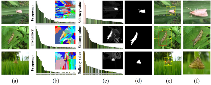
In the original set of images we observed that pest insect objects usually occupy highly contrast color regions relative to their backgrounds (Fig. 1(a)). Many physiological experiments and computer vision models have proved such regions have a higher so-called saliency value than that of their surroundings, which is an important step for the object detection42,43. Thus we applied a recently developed approach “global contrast based salient region detection”40 to automatically localize the regions of pest insects in given images, as detailed below.
Figure 1. Examples of constructing Pest ID.
(a) original images, in which the first and the third rows are provided by Guoguo Yang, and the second row courtesy of Keiko Kitada. (b) segmented regions and the corresponding color histograms. (c) saliency maps and saliency value of each region. (d) GrabCut45 segmentation results initialized from the thresholded saliency maps. (e) localization results, in which tight bounding boxes (red) containing pest insect objects are extended to squares (yellow). (f) Pest ID images.
Shown in Fig. 1, the original images (Fig. 1(a)) are first segmented into regions using a graph-based image segmentation method44, and then color histograms are built for each region (Fig. 1(b)). Due to the efficiency requirement, each color channel (RGB) of the given images is quantized to have 10 different values, which reduces the number of all colors to 103. For each region rk, the saliency value S(rk) is computed to represent its contrast to others,
 |
Where,
 |
where ω(ri) is the number of pixels in ri, Ds and Dr are respectively the spatial distance and color space distance metric between two regions, and σs controls the strength of the spatial weighting. For each region rk, its salience value benefits from its spatial distance to all other regions, and here a large value of σs (0.45) is used to reduce the effect of this spatial weighting so that contrast to father regions would contribute more to the saliency value of current region. Note that in Dr, based on the color histogram (Fig. 1(b)), the probability p(cm,i) of each color cm,i among all nm colors in the m-th region rm is considered for the original color distance D, m = 1, 2, giving more weight to the dominate color difference. These steps are used to obtain the maps (Fig. 1(c)) indicating the saliency value of each region. We can see from these saliency maps that the regions representing pest insect objects are of higher value compared to background.
GrabCut based localizatiohn
The computed saliency maps are then used to assist a segmentation of pest insect objects, a key step to the subsequent localization. A GrabCut45 algorithm is initialized using a segmentation obtained by thresholding the saliency maps using a fixed threshold th (0.3) which is chosen experimentally to give the localization accuracy of over 0.9 in a subset of the original images (see details in section Localization Accuracy of Saliency Detection). After initialization, an iteration of 3 times of GrabCut is performed, which gives the final results of the rough segmentation of pest insect objects (Fig. 1(d)). With these segmentation results, the bounding boxes containing the pest insect objects are extended as squares (Fig. 1(e)), and then cropped from their original images. Finally, all cropped regions are resized as 256 × 256 (Fig. 1(f)) for constructing the standard database Pest ID. Details of Pest ID are shown in Table 1, and its online application is being built.
Table 1. Details of Pest ID.
| Species | Cnaphalocrocis medinalis | Chilo suppressalis | Parnara Guttata | Nilaparvata lugens | Nephotettix cincticeps | Diamondback moth |
| Quantity | 480 | 485 | 481 | 399 | 370 | 554 |
| Species | Scirpophaga incertulas | Oxya chinensis | Naranga aenescens | Ostrinia rnacalis | Sogatella furcifera | Cletus punctiger |
| Quantity | 520 | 400 | 381 | 401 | 183 | 482 |
Deep Convolutional Neural Network
Overall Architecture
We implemented and altered the net architecture (Fig. 2) based on AlexNet36. This 8-layer CNN network can be thought of as a self-learning progression of local image features from low to mid to high level. The first five layers are called convolutional layers (Conv1-5), in which the higher layers synthesize more complex structural information across larger scales sequences of convolutional layers. Interleaved with the max pooling, they are capable of capturing deformable parts, and reducing the resolution of the convolutional output. The last two fully connected layers (FC6, FC7) can capture complex co-occurrence statistics, which drop semantics of spatial location. A final classification layer accepts the previous representation vector for the recognition of a given image. This architecture is appropriate for learning powerful local features from the complex natural image dataset46. A schematic of our model is presented below (see reference36 for more network architecture details).
Figure 2. Overall architecture of the model.
After saliency detection, a 227 × 227 crop of the localized image is presented as the input. It is convolved in the first convolutional layer (Conv1) with local receptive fields, using a convolutional stride of fixed step. The results are then represented in vector form through other 4 convolutional layers (Conv2–5) which are with 3 max pooling layers, and two fully connected layers (FC6, FC7). The final layer is a 12-way softmax function for classification. Original image courtesy of Junfeng Gao.
Training the Deep Convolutional Neural Network
Each input image is processed as 256 × 256 as previously. 5 random crops (and their horizontal mirrors) of size 227 × 227 pixels are presented to the model in mini-batches of 128 images. Each convolutional layer is followed by rectification non-linearities (ReLU) activation, and max pooling are located after the first (Conv1), second (Conv2) and fifth (Conv5) convolutional layers. The last layer (classification layer) has 12 output units corresponding to 12 categories, upon which a softmax loss function is placed to produce the loss for back-propagation. The initial weights in the net are drawn from a Gaussian distribution with zero mean with a standard deviation of 0.01. They are then updated by stochastic gradient descent, accompanied by momentum term of 0.8 and the L2-norm weight decay of 0.005. The learning rate is initially 0.01 and is successively decreased by a factor of 10 during 3 epochs, each of which consists of 20000 iterations. We trained the model on a single NVIDIA GTX 970 4GB GPU equipped on a desktop computer with a Intel Core i7 CPU and 16GB memory.
Dropout
Overfitting is a serious problem in a network with a large set of parameters (about 60 million). The 12 classes in Pest ID used only 10 bits of constraint on the mapping from image to label, which could allow significant generation error47. Dropout41 is a powerful technique to address this issue when data is limited. This works by randomly removing net units at a fixed probability during training, and by using a whole architecture at test time. This counts as combining different “thinned” subnets for improving the performance of the overall architecture.
Experiment and Analysis
Localization Accuracy of Saliency Detection
Thresholded saliency maps present the initial regions for GrabCut45 segmentation and thus determine the final localization results. In order to comprehensively evaluate the effects of different threshold th on the localization accuracy, we varied this parameter from 0.1 to 0.9 in steps of 0.1. Note that in this evaluation, the correct localization result on each original image is defined by two restrictions: (1) the area difference between the localization box and the ground truth box less than 20% of the latter, (2) at least 80% localization region pixels belong to that of the ground truth region. The ground truth boxes of all original images were manually labelled before.
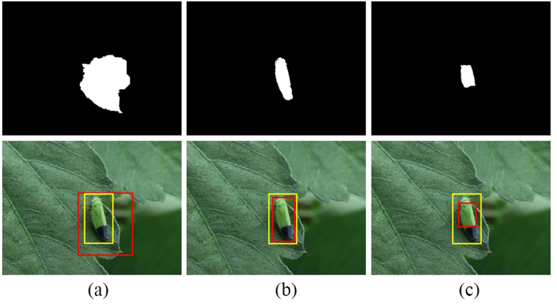
As shown in Fig. 3, the localization accuracy curve achieves its maximal value at the point of 0.3 where over 90% of localization results meet above restrictions. The visual comparison (see Fig. 4) illustrates that lower threshold values capture too much unwanted background (Fig. 4(a)), while one that is too high might be unable to highlight the whole target object (Fig. 4(c)). At the optimal point, there remains a fraction of pest objects that are not detected. We investigated these failure cases, and found that most of them could be attributed to the high background bokeh in the original images; when both the pest insect and their nearby regions are of high contrast to the distant regions, they have similar saliency. This can result in undesirable thresholded saliency maps including too many unwanted initial regions, making GrabCut difficult to segment pest insect objects.
Figure 3. Localization accuracy under different threshold th.
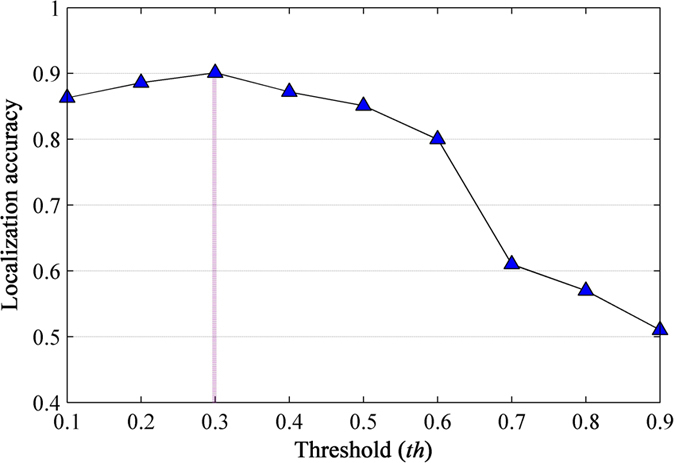
Figure 4. An example for visual comparison of localization results at different threshold th.
(a) th = 0.1. (b) th = 0.3. (c) th = 0.5. Column 1: Thresholded saliency maps. Column 2: The ground truth boxes (yellow) and localization boxes (red) in the original images. Original image for this example courtesy of Masatoshi Ohsawa.
Despite the weakness in the above special cases, this approach is still expected to be a promising tool for pest insect localization due to its low computation cost and simplicity40, which will be beneficial for practical applications. In the future, we plan to increase detection, using exhaustive search39 or selective search48, in the resulting saliency maps. This is necessary for generalizing the localization ability of saliency detection, and extension of the Pest ID database to contain more pest insect species.
Optimization of the Overall Architecture
The overall architecture includes a number of sensitive parameters and optimization strategies that can be changed: (i) size, number, and convolutional stride of the local receptive fields, (ii) dropout ratio for the fully-connected layers, and (iii) the loss function in the final classification layer. In this section, we present our experimental results testing the impact of these factors on performance.
The Role of the Local Receptive Fields
Size of local receptive fields
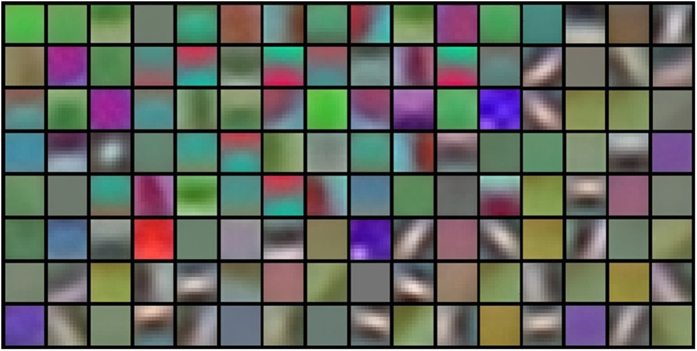
Local receptive fields are actually the filters in the first layer (see Fig. 2). Their size is usually considered to be the most sensitive parameter, upon which all the following works are built49. The ordinary choice of this parameter is in the range of 7 × 7 to 15 × 15 when the image size is around 200 × 20050. In this experiment, we ascertained that 11 × 11 works best for Pest ID images (see Fig. 5). The reason might be that the pest objects have similar scales and thus are rich in both structure and texture information. Normally, small receptive fields focus on capturing texture variation, while large ones tend to match structure differences. In this regard, our selected filters achieved the balance between these tendencies. For example, a round-shaped image patch can be recognized as an eye or spots using a suitable receptive field, but this recognition might be infeasible at a smaller or larger size. As illustrated in Fig. 6, these filters tend to produce biologically plausible feature detectors like subparts of pest insects.
Figure 5. Effects of size and number of local receptive fields (first layer filters) on the validation accuracy.
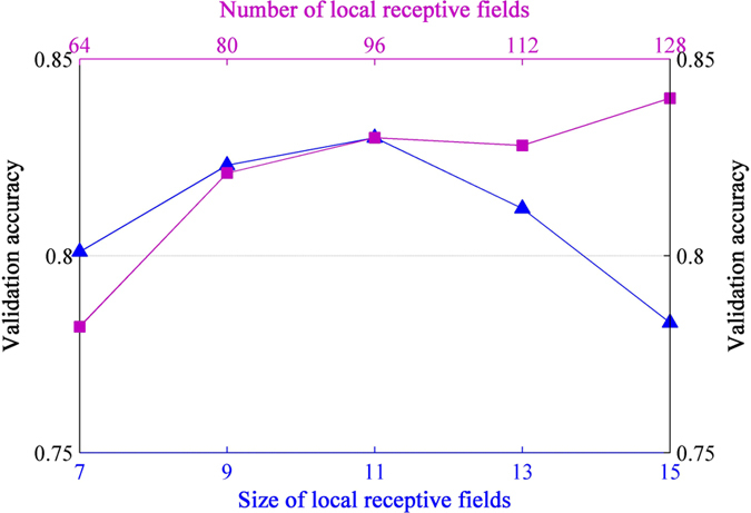
The testing of number of local receptive fields was based on their size being 11 × 11. About 25% of the images from each species in Pest ID were randomly selected for constructing the validation set, totaling 1210 images.
Figure 6. Visualization of local receptive fields.
128 local receptive fields of size 11 × 11 are projected to pixel space.
Number of local receptive fields
A reasonable deduction could be that the net uses significantly fewer receptive fields than AlexNet36, because we have fewer classes compared to other tasks like Imagenet51. Unexpectedly, we still found that more local receptive fields led to better performance (Fig. 5). A possible explanation is that pest objects lack consistency in the same class due to the intra-class variability and the viewing angles (pose) difference. Thus more receptive fields are needed to ensure that enough variants for the same species can be captured.
Convolutional stride
The convolutional stride s used in the net is the spacing between local image patches where feature values are extracted (see Fig. 2). This parameter is frequently discussed in convolutional operations49. DCNNs normally use a stride s > 1 because computing feature mapping is very expensive during training. We fixed the number of local receptive fields (128) and their size (11 × 11), and varied the stride over (2, 3, 4, 5, 6, 7) pixels, to investigate how much performance compromise costs in terms of time. Shown in Fig. 7, both validation accuracy and time cost show a clear downward trend with increasing step size as expected. For even a stride of s = 3, we suffered a loss of 3% accuracy, and saw bigger effects when using the larger ones. To achieve the trade-off with time cost, we adopted s = 3 that confers the smallest change in validation accuracy without significantly increasing the time of training.
Figure 7. Effects of different convolutional stride of local receptive fields on validation accuracy and the corresponding time cost.
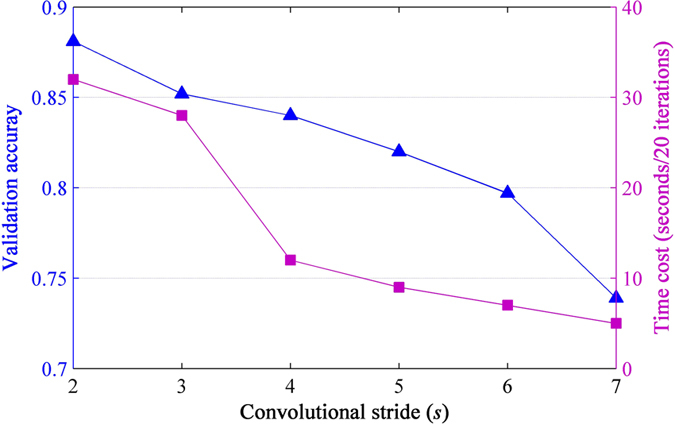
The time is calculated for 20 iterations.
Effects of Dropout Ratio
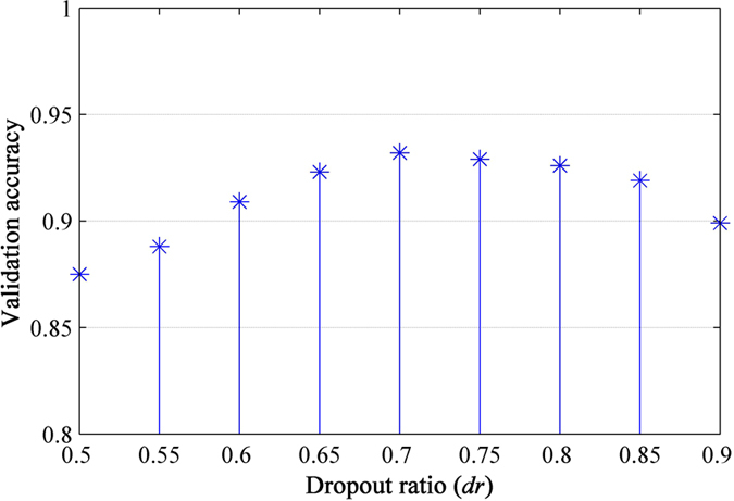
Dropout has a tunable hyperparameter dropout ratio dr (the probability of deactivating a unit in the network)41. A large dr therefore means very few units will turn on during training. In this section, we explored the effect of varying this hyperparameter within the range between 0.5 and 0.9 which is most recommended41. In Fig. 8, we see that as dr increases, the error decreases. It becomes flat when 0.65 ≤ dr ≤ 0.8 and then increases as dr approaches 1. Since dropout can be seen as an approximate model combination, a higher dropout ratio implies that more submodels are used. Thus, the network performs better at a large dr (such as 0.7). However, a too aggressive dropout ratio would lead to a network lacking sufficient neurons to model the relationship between the input and the correct output (such as dr = 0.9).
Figure 8. Effect of changing the dropout ratio on resulting validation accuracy.
Effects of the Loss function
The most popular loss functions used with DCNNs are logistic, softmax and hinge loss52. Here we investigated the effectiveness of softmax vs hinge (one-versus-all) for training (since logistic function is a derivative of softmax53, we did not test it here). Both functions were tested using the same learning setting (size, number and stride of local receptive fields of 11, 128 and 3, and a dropout ratio of 0.7), and a large L2-norm weight decay constant of 0.005 to prevent overfitting. Under these conditions, softmax slightly outperformed hinge loss (0.932 vs. 0.891 in validation accuracy). To explicitly illustrate the advantage of softmax, we plotted the learning procedures of these two functions in Fig. 9. It can be seen that learning with softmax allowed better generalization (similar training error but much smaller validation error than hinge), and converged faster.
Figure 9. Training and validation errors for hinge loss (one-versus-all) or softmax loss as learning proceeds.
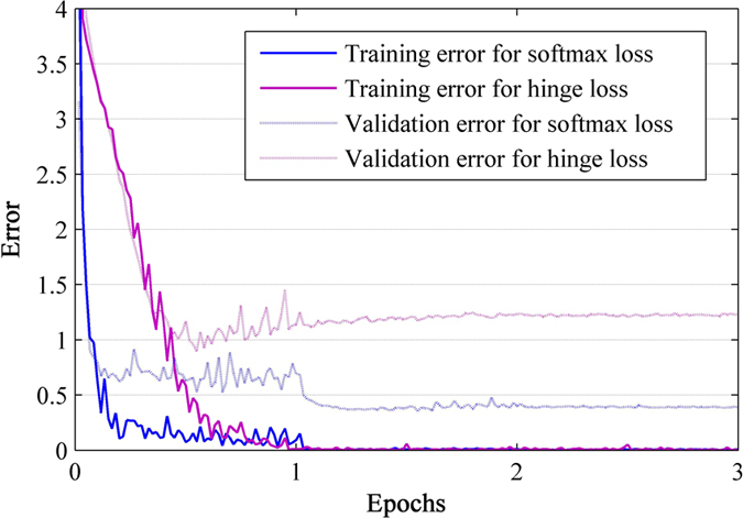
The errors were computed over 3 epochs, of which each has 20000 iterations. Both learning processes used the same local receptive fields and drop ratio. The two loss functions were associated with a large L2-norm weight decay constant 0.005 (larger than that used in AlexNet36), which has proved to be useful for improving generalization of neural networks55. Under these settings, softmax and hinge respectively achieved 0.932 and 0.891 in validation accuracy.
Although on the Pest ID database softmax shows better results, this should now be adopted as the standard loss as our tested parameters are too limited. If Pest ID is augmented to include significantly more species, it will be necessary to re-address this issue.
Practical Utility of the Model
From a practical standpoint, use of this strategy for paddy field applications requires that the model can execute in real-time and achieve rapid retraining by accepting new samples or additional classes. It is desirable, therefore, to seek approaches to speed up the models while still retaining a high level of performance. In this section, we focus on structural changes in the above overall architecture that enable faster running times with small effects on performance. In Table 2, we analyzed the performance and the corresponding runtime of our model by shrinking its depth (number of layers) and width (filters in each layer).
Table 2. Effects of changing the overall architecture on performance and runtime.
| Type Index | Architectural Change | Training Time/Speedup | Processing Rate/Speedup | Validation Accuracy |
|---|---|---|---|---|
| 1 | Overall architecture | 13.9 h/1.0× | 3.88 ms/1.0× | 0.932 |
| 2 | Removed layer FC7 | 12.8 h/1.1× | 3.40 ms/1.1× | 0.908 |
| 3 | Removed layers FC6, 7 | 12.5 h/1.1× | 3.05 ms/1.3× | 0.897 |
| 4 | Removed layers FC6, 7, Conv5 | 10.1 h/1.4× | 2.45 ms/1.6× | 0.869 |
| 5 | Removed layers FC6, 7, Conv4, 5 | 9.5 h/1.5× | 1.78 ms/2.2× | 0.724 |
| 6 | Removed layers FC6, 7, Conv3, 4, 5 | 6.6 h/2.1× | 1.66 ms/2.3× | 0.633 |
| 7 | Removed layers FC6, 7, Conv2, 3, 4, 5 | 3.1 h/4.5× | 1.65 ms/2.3× | 0.630 |
| 8 | Adjust Layers Conv2, 3, 4, 5: 192, 320, 320, 192 filters | 12.0 h/1.2× | 3.48 ms/1.1× | 0.929 |
| 9 | Adjust Layers Conv2, 3, 4, 5: 128, 256, 256, 128 filters | 9.2 h/1.5× | 2.84 ms/1.4× | 0.924 |
| 10 | Adjust Layers Conv2, 3, 4, 5: 64, 192, 192, 64 filters | 7.1 h/2.0× | 2.28 ms/1.7× | 0.917 |
The processing rate indicates the time of a feed-forward pass for one image. Speedup denotes the time ratio of the changed architectures versus the overall architecture.
Ablation of entire layers
We first explored the robustness of the overall architecture by completely removing each layer. As shown in Table 2, removing the fully-connected layers (Type-2, 3) made only a slight difference to the overall architecture. This is surprising, because these layers contain almost 90% of the parameters. Removing the top convolutional layers (Tpye-4) also had little impact. However, removing the intermediate convolutional layers (Type-5, 6, 7) resulted in a dramatic decrease in both accuracy and runtime. This suggests that the intermediate convolutional layers (Conv2, Conv3, Conv4) constitute the main part of the computational resource, and their depth is important for achieving good results. If a relatively lower level of accuracy is acceptable in practical applications, Type-4 architecture would be the best choice.
Adjusting the size of each convolutional layers
We then investigated the effects of adjusting the sizes of all convolutional layers except the first one, discussed previously. In Table 2, the filters in each convolutional layer were reduced by 64 each time. Surprisingly, all architectures (Type-8, 9, 10) showed significant decreases in running time with relatively small effects on performance. Especially notable is Type-10 architecture that, with a rather small margin the overall architecture (0.932 vs. 0.917), proceeds about 2.0× faster in training and 1.7× faster in processing rate than the overall architecture. This means redundant filters exist in the intermediate convolutional layers, and a smaller net is sufficient to substitute for the overall architecture, which will enhance the practical utility of the model.
In addition to runtime, another critical component of our models is the ability to implement online learning as accepting unlabeled new samples in the fields. There are multiple components for this process, such as reducing the size of mini-batch (extremity is 1), updating model parameters with samples of low confidence (output of the classification layer)54, just retraining the final classification layer, or constructing a sparse auto-encoder to obtain sparse features that allow an effective pre-training on a large dataset consisting of more species as possible (such as additional classes not included in our task) and replacing the model parameters online49. Many alternative strategies are available, and evaluation of these alternatives will be the focus of the future work.
Comparison with Other Methods
In Table 3, we compared our models (Type-1, Type-10) with previous methods on the test set provided by the Department of Plant Protection, Zhejiang University. This dataset contains 50 images for each class, is evenly distributed, thus the mAP (mean average precision) is an indicator of the classification accuracy. We performed this comparison as follows:
Table 3. Comparison of DCNNs with other methods on the same dataset.
Comparison with AlexNet
AlexNet36 was pretrained on the Imagenet51 database and fine-tuned in our experiment. In training and testing with this model, we did not adopt localization but instead resized all the original images to 256 × 256. As shown in Table 3, mAP of AlexNet reaches an accuracy of 0.834. By combining this with saliency map based localization, both our models achieved vastly better performance, 0.923 and 0.951. Obviously, the localization procedure substantially reduced the number of potential false positives in background.
Comparison with traditional methods
we selected three traditional methods20,22,23 for comparison with our DCNN pipeline, and have summarized the results and the key techniques for the different methods in Table 3. All models were trained with Pest ID images, and evaluated on the localized test images. We found that our method allowed improvement of at least 0.1 over the other models, conforming the effectiveness of DCNNs to extract and organize the discriminative information.
The effectiveness of DCNN
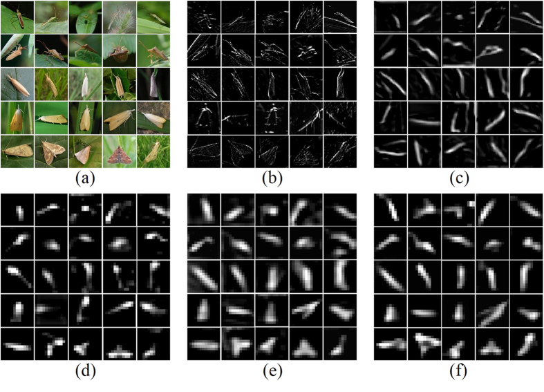
to understand how the steps of our process achieved better performance, we visualized the feature maps with the strongest activation from each layer of the overall architecture to look inside its internal operation and behavior, as shown in Fig. 10. The original images that have been localized are shown prior to the levels of image processing and analysis. Layer 1 responds to edges or corners and layer 2 performs the conjunctions of these edges. Layer 3 allows more complex invariances, capturing distinctive textures. Layer 4 and layer 5 roughly cover the entire objects, but the latter is more robust in distinguishing the objects from the irrelevant backgrounds. The visualization clearly demonstrates the effectiveness of DCNN in handling significant pose variation (rows 1, 2), inter-classes similarity (rows 3, 4) or intra-class variability (row 5).
Figure 10. Visualization of feature maps in the overall architecture.
(a) A subset of original images, which had been performed on a localization processing, were selected from the test set for illustrating pose variations (Row 1&2), inter-species similarity (Row 3&4) and intra-class difference (Row 5). These images were then used in our recognition tasks, and in (b–f), we show the top activated feature maps of the corresponding original images after layers Conv1–5. The brightness and contrast were enhanced for each feature map for the best view. Original images are provided by Huan Zhang.
Conclusion and future work
We have demonstrated the effectiveness of using a saliency map-based approach for localizing pest insect objects in natural images. We applied this strategy to internet images and constructed a standard database Pest ID for training DCNNs. This database has unprecedented scale and thus significantly is enriched for the variation of each species. This allows the construction of powerful DCNNs for pest insect classification. We also proved a large DCNN can retain satisfactory performance with great reduction to its architecture, required for practical application. The pipeline of both localization and classification was not used previously and thus we are the first to report this strategy for a pest insect classification task.
Our approach can be improved further. (1) Including a finer search in the saliency maps may improve the localization accuracy, and is beneficial for expanding Pest ID to include significantly more species in the future. (2) Online learning could be implemented to make use of unlabeled new samples in the field for updating the model parameters. (3) The difficulty in interpretation when object overlapping occurs remains a challenge that will need to be addressed to allow the practical application of this design.
Additional Information
How to cite this article: Liu, Z. et al. Localization and Classification of Paddy Field Pests using a Saliency Map and Deep Convolutional Neural Network. Sci. Rep. 6, 20410; doi: 10.1038/srep20410 (2016).
Acknowledgments
This study was supported by 863 National High-Tech Research and Development Plan (project no: 2013AA102301), Natural Science Foundation of China (project no: 31471417) and the Fundamental Research Funds for the Central Universities. We acknowledge Keiko Kitada and Masatoshi Ohsawa for granting permission to use their images in this paper.
Footnotes
Author Contributions Z.L. wrote the main manuscript text. G.Y. prepared Figure 1; J.G. prepared Figure 2; Z.L. prepared Figure 3–10, and he also prepared Table 1–3. H.Z. provided the pest insects images in the test dataset. Y.H. designed the study. All authors reviewed the manuscript.
References
- Estruch J. J. et al. Transgenic plants: an emerging approach to pest control. Nat. Biotechnol 15, 137–141 (1997). [DOI] [PubMed] [Google Scholar]
- Parsa S. et al. Obstacles to integrated pest management adoption in developing countries. Proc Natl Acad Sci USA 111, 3889–3894 (2014). [DOI] [PMC free article] [PubMed] [Google Scholar]
- Metcalf R. L. & Luckmann W. H. In Introduction to insect pest management 3rd edn (eds Metcalf R. L. et al.) Ch. 1, 1–34 (Wiley, 1994). [Google Scholar]
- Hashemi S. M., Hosseini S. M. & Damalas C. A. Farmers’ competence and training needs on pest management practices: Participation in extension workshops. Crop. Prot 28, 934–939 (2009). [Google Scholar]
- Boissard P., Martin V. & Moisan S. A cognitive vision approach to early pest detection in greenhouse crops. Comput. Electron. Agr 62, 81–93 (2008). [Google Scholar]
- Hassan S. N. A., Rahman N. N. S. A. & Zaw Z. Vision based entomology: a survey. International Journal of Computer Science & Engineering Survey 5, 19–31(2014). [Google Scholar]
- Sarpola M. et al. An aquatic insect imaging system to automate insect classification. Transactions of the ASABE 51, 2217–2225 (2008). [Google Scholar]
- Bengio Y. & LeCun Y. In Large-scale kernel machines (eds Bottou L. et al.) Ch. 14, 321–358 (MIT Press, 2007). [Google Scholar]
- Zhu L. & Zhang Z. Auto-classification of insect images based on color histogram and GLCM. Paper presented at The 7th International Conference on Fuzzy Systems and Knowledge Discovery (FSKD 2010), Yantai, China. Los Alamitos: IEEE. (2010, August 10–12).
- Solis-Sánchez L. O., García-Escalante J., Castañeda-Miranda R., Torres-Pacheco I. & Guevara-González R. Machine vision algorithm for whiteflies (Bemisia tabaci Genn.) scouting under greenhouse environment. J APPL ENTOMOL 133, 546–552 (2009). [Google Scholar]
- Zhang H. & Mao H. Feature selection for the stored-grain insects based on PSO and SVM. Paper presented at 2009 2nd International Workshop on Knowledge Discovery and Data Mining (WKDD 2009), Moscow, Russia. Los Alamitos: IEEE. (2009, January 23–25).
- Yang H. et al. Research on insect identification based on pattern recognition technology. Paper presented at 2010 6th International Conference on Natural Computation (ICNC 2010), Yantai, China. Los Alamitos: IEEE. (2010, August 10–12).
- O’Neill M., Gauld I., Gaston K. & Weeks P. Daisy: an automated invertebrate identification system using holistic vision techniques. Paper presented at The Inaugural Meeting of the BioNET-INTERNATIONAL Group for Computer-Aided Taxonomy (BIGCAT), Cardiff, Welsh. Surrey: BioNet-INTERNATIONAL Technical Secretariat. (1997, July 2–3).
- Do M., Harp J. & Norris K. A test of a pattern recognition system for identification of spiders. B. Entomol. Res 89, 217–224 (1999). [Google Scholar]
- Yu Z. & Shen X. Application of Several Segmentation Algorithms to the Digital Image of Helicoverpa armigera. Journal of China Agricultural University 5, 012 (2001). [Google Scholar]
- Arbuckle T., Schroder S., Steinhage V. & Wittmann D. Biodiversity informatics in action: identification and monitoring of bee species using ABIS. Paper presented at The 15th International Symposium Informatics for Environmental Protection, Zurich, Switzerland. Marburg: Metropolis-Verlag. (2001, October 10–12).
- Yao Q. et al. An insect imaging system to automate rice light-trap pest identification. J INTEGR AGR 11, 978–985 (2012). [Google Scholar]
- Kumar R., Martin V. & Moisan S. Robust insect classification applied to real time greenhouse infestation monitoring. Paper presented at The 20th International Conference on Pattern Recognition: Visual Observation and Analysis of Animal and Insect Behavior Workshop (VAIB 2010), Istanbul, Turkey. Los Alamitos: IEEE. (2010, August 22).
- Solis-Sánchez L. O. et al. Scale invariant feature approach for insect monitoring. Comput. Electron. Agr 75, 92–99 (2011). [Google Scholar]
- Cheng L. & Guyer D. Image-based orchard insect automated identification and classification method. Comput. Electron. Agr 89, 110–115 (2012). [Google Scholar]
- Xia C., Lee J., Li Y., Chung B. & Chon T. In situ detection of small-size insect pests sampled on traps using multifractal analysis. Opt. Eng 51, 027001-1-027001-12 (2012). [Google Scholar]
- Venugoban K. & Ramanan A. Image classification of paddy field insect pests using gradient-based features. International Journal of Machine Learning and Computing 4, 1 (2014). [Google Scholar]
- Zhang J., Wang R., Xie C. & Li R. Crop pests image recognition based on multifeatures fusion. Journal of Computational Information Systems 10, 5121–5129 (2014). [Google Scholar]
- Yao Q. et al. Automated counting of rice planthoppers in paddy fields based on image processing. J INTEGR AGR 13, 1736–1745 (2014). [Google Scholar]
- Sivic J. & Zisserman A. Video Google: a text retrieval approach to object matching in videos. Paper presented at 2003 9th International Conference on Computer Vision (ICCV 2003), Nice, France. Los Alamitos: IEEE. (2003, October 13–16).
- Ojala T., Pietikäinen M. & Mäenpää T. Multiresolution gray-scale and rotation invariant texture classification with local binary patterns. IEEE T PATTERN ANAL 24, 971–987 (2002). [Google Scholar]
- Lowe D. G. Distinctive image features from scale-invariant keypoints. Int. J. Comput. Vision 60, 91–110 (2004). [Google Scholar]
- Dalal N. & Triggs B. Histograms of oriented gradients for human detection. Paper presented at 2005 IEEE Computer Society Conference on Computer Vision and Pattern Recognition (CVPR 2005), San Diego, California, USA. Los Alamitos: IEEE. (2005, June 20–25).
- Andreopoulos A. & Tsotsos J. K. 50 Years of object recognition: directions forward. Comput. Vis. Image Und 117, 827–891 (2013). [Google Scholar]
- Zhang W., Deng H., Dietterich T. G. & Mortensen E. N. A hierarchical object recognition system based on multi-scale principal curvature regions. Paper presented at 2006 18th International Conference on Pattern Recognition (ICPR 2006), Hong Kong, China. Los Alamitos: IEEE. (2006, August 20–24).
- Larios N. et al. Automated insect identification through concatenated histograms of local appearance features: feature vector generation and region detection for deformable objects. Mach. Vision. Appl 19, 105–123 (2008). [Google Scholar]
- Lu A., Hou X., Liu C. L. & Chen X. Insect species recognition using discriminative local soft coding. Paper presented at 2012 21st International Conference on Pattern Recognition (ICPR 2012), Tsukuba, Japan. Los Alamitos: IEEE. (2012, November 11–15).
- Lytle D. A. et al. Automated processing and identification of benthic invertebrate samples. J. N. Am. Benthol. Soc 29, 867–874 (2010). [Google Scholar]
- Bengio Y., Courville A. & Vincent P. Representation learning: a review and new perspectives. IEEE T PATTERN ANAL 35, 1798–1828 (2013). [DOI] [PubMed] [Google Scholar]
- Güçlü U. & Van G. M. A. Deep neural networks reveal a gradient in the complexity of neural representations across the brain’s ventral visual pathway. arXiv preprint arXiv:1411.6422 (2014).
- Krizhevsky A., Sutskever I. & Hinton G. E. Imagenet classification with deep convolutional neural networks. Advances in Neural Information Processing Systems, 25, 1097–1105 (2012). [Google Scholar]
- Karpathy A. et al. Large-scale video classification with convolutional neural networks. Paper presented at 2014 IEEE Computer Society Conference on Computer Vision and Pattern Recognition (CVPR 2014), Columbus, Ohio, USA. Los Alamitos: IEEE. (2014, June 24–27).
- Lee C., Xie S., Gallagher P., Zhang Z. & Tu Z. Deeply-supervised nets. arXiv preprint arXiv:1409.5185 (2014).
- Sermanet P. et al. Overfeat: Integrated recognition, localization and detection using convolutional networks. arXiv preprint arXiv:1312.6229 (2013).
- Cheng M., Mitra N. J., Huang X., Torr P. H. & Hu S. Global contrast based salient region detection. IEEE T PATTERN ANAL 37, 569–582 (2015). [DOI] [PubMed] [Google Scholar]
- Srivastava N., Hinton G. H., Krizhevsky A., Sutskever I. & Salakhutdinov R. Dropout: a simple way to prevent neural networks from overfitting. J MACH LEARN RES 15, 1929–1958 (2014). [Google Scholar]
- Han J., Ngan K. N., Li M. & Zhang H. Unsupervised extraction of visual attention objects in color images. IEEE T CIRC SYST VID 16, 141–145 (2006). [Google Scholar]
- Ko B. C. & Nam J. Y. Object-of-interest image segmentation based on human attention and semantic region clustering. JOSA A 23, 2462–2470 (2006). [DOI] [PubMed] [Google Scholar]
- Felzenszwalb P. F. & Huttenlocher D. P. Efficient graph-based image segmentation. Int. J. Comput. Vision 59, 167–181 (2004). [Google Scholar]
- Rother C., Kolmogorov, V. & Blake A. Grabcut: interactive foreground extraction using iterated graph cuts. ACM T GRAPHIC 23, 309–314 (2004). [Google Scholar]
- Razavian A. S., Azizpour H., Sullivan J. & Carlsson S. CNN features off-the-shelf: an astounding baseline for recognition. Paper presented at 2014 IEEE Computer Society Conference on Computer Vision and Pattern Recognition (CVPR 2014), Columbus, Ohio, USA. Los Alamitos: IEEE. (2014, June 24–27).
- Valiant L. G. A theory of the learnable. Commun. Acm 27, 1134–1142 (1984). [Google Scholar]
- Girshick R., Donahue J., Darrell T. & Malik, J. Rich feature hierarchies for accurate object detection and semantic segmentation. Paper presented at 2014 IEEE Computer Society Conference on Computer Vision and Pattern Recognition (CVPR 2014), Columbus, Ohio, USA. Los Alamitos: IEEE. (2014, June 24–27).
- Coates A., Ng A. Y. & Lee H. An analysis of single-layer networks in unsupervised feature learning. Paper presented at The 14th International Conference on Artificial Intelligence and Statistics (AISTATS 2011), Ft. Lauderdale, Florida, USA. New York: Springer. (2011, April 11–13).
- Yang Y. & Hospedales T. M. Deep neural networks for sketch recognition. arXiv preprint arXiv:1501.07873 (2015).
- Deng J. et al. Imagenet: a large-scale hierarchical image database. Paper presented at 2009 IEEE Computer Society Conference on Computer Vision and Pattern Recognition (CVPR 2009), Miami, Florida, USA. Los Alamitos: IEEE. (2009, June 20–26).
- Jia Y. et al. Caffe: convolutional architecture for fast feature embedding. Paper presented at The 22nd ACM International Conference on Multimedia (ACMMM 2014), Orlando, Florida, USA. New York: ACM. (2014, November 3–7).
- Arribas J. I., Cid-Sueiro J., Adali T. & Figueiras-Vidal A. R. Neural architectures for parametric estimation of a posteriori probabilities by constrained conditional density functions. Paper presented at Neural Networks for Signal Processing IX: The 1999 IEEE Signal Processing Society Workshop, Madison, Wisconsin, USA. Los Alamitos: IEEE. (1999, August 23–25).
- Peemen M., Mesman B. & Corporaal C. Speed sign detection and recognition by convolutional neural networks. Paper presented at The 8th International Automotive Congress (IAC 2011), Eindhoven, Netherlands. Eindhoven: Technische Universiteit Eindhoven. (2011, May 16–17).
- Jeong S. & Lee S. Adaptive learning algorithms to incorporate additional functional constraints into neural networks. Neurocomputing 35, 73–90 (2000). [Google Scholar]


