Clinical Prediction Models for Sleep Apnea: The Importance of Medical History over Symptoms

Abstract

Study Objective:

Obstructive sleep apnea (OSA) is a treatable contributor to morbidity and mortality. However, most patients with OSA remain undiagnosed. We used a new machine learning method known as SLIM (Supersparse Linear Integer Models) to test the hypothesis that a diagnostic screening tool based on routinely available medical information would be superior to one based solely on patient-reported sleep-related symptoms.

Methods:

We analyzed polysomnography (PSG) and self-reported clinical information from 1,922 patients tested in our clinical sleep laboratory. We used SLIM and 7 state-of-the-art classification methods to produce predictive models for OSA screening using features from: (i) self-reported symptoms; (ii) self-reported medical information that could, in principle, be extracted from electronic health records (demographics, comorbidities), or (iii) both.

Results:

For diagnosing OSA, we found that model performance using only medical history features was superior to model performance using symptoms alone, and similar to model performance using all features. Performance was similar to that reported for other widely used tools: sensitivity 64.2% and specificity 77%. SLIM accuracy was similar to state-of-the-art classification models applied to this dataset, but with the benefit of full transparency, allowing for hands-on prediction using yes/no answers to a small number of clinical queries.

Conclusion:

To predict OSA, variables such as age, sex, BMI, and medical history are superior to the symptom variables we examined for predicting OSA. SLIM produces an actionable clinical tool that can be applied to data that is routinely available in modern electronic health records, which may facilitate automated, rather than manual, OSA screening.

Commentary:

A commentary on this article appears in this issue on page 159.

Citation:

Ustun B, Westover MB, Rudin C, Bianchi MT. Clinical prediction models for sleep apnea: the importance of medical history over symptoms. J Clin Sleep Med 2016;12(2):161–168.

INTRODUCTION

Obstructive sleep apnea (OSA) is a treatable contributor to morbidity and mortality, as well as decreased performance and quality of life.^1–3 However, most patients with OSA remain undiagnosed.^4,5 Although recent advances in home sleep diagnostics may increase access to testing, limitations in the accuracy of these devices prompted the American Academy of Sleep Medicine to state explicitly home test kits are not appropriate for general screening.^6,7 Thus, in many cases, recognition of OSA risk comes either from patient reported symptoms or physician suspicion. This pathway of clinical suspicion may itself be a reason for under-recognition, as the “classic” symptoms and signs of OSA are not strongly predictive of the presence or severity of OSA. For example, the often-utilized Epworth Sleepiness Scale carries minimal predictive value for OSA measures or objective sleepiness measures.^8–10 Other screening tests using a variety of measures have shown improvements over the Epworth,¹¹ but even the best-validated scale recently gaining interest, the “STOP-BANG,” has important limitations when used in screening, depending on the pretest probability of OSA.¹² Most scales focus on symptoms such as snoring, nocturnal gasping, witnessed apneas, and sleepiness or other daytime complaints. Despite the apparent face validity of these factors, even expert clinical impression has weak sensitivity and specificity (< 70% each) for predicting OSA.¹³ In contrast, certain comorbidities may carry important information, perhaps more important than symptoms themselves. For example, patients with uncontrolled hypertension may have a very high risk of OSA, upwards of 80%.¹⁴ OSA risk prediction models that utilize demographic and comorbidity information are advantageous in that they can make predictions from electronic health records without drawing on the limited resources available for direct patient care encounters.

BRIEF SUMMARY

Current Knowledge/Study Rationale: Most screening tools for OSA rely on a combination of medical history components as well as self-reported symptoms. The relative contributions of each of these two categories to the predictive utility is not well understood.

Study Impact: The current results suggest that self-reported symptoms contribute little information beyond that which is contained in the medical history. As medical history components may be extractable from electronic records, future screening tools may be amenable to scalable automation.

We set out to identify which combinations of patient features, drawn from a large set of candidates, are predictive of OSA. To this end, we took advantage of a new machine learning method known as a Supersparse Linear Integer Models (SLIM). SLIM produces data-driven medical scoring systems that are accurate yet simple, such that predictions can be made without the use of a calculator or computer.¹⁵ We tested the hypothesis that predictive models created from symptom features would differ in OSA prediction performance from predictive models created from non-symptom features.

METHODS

Database

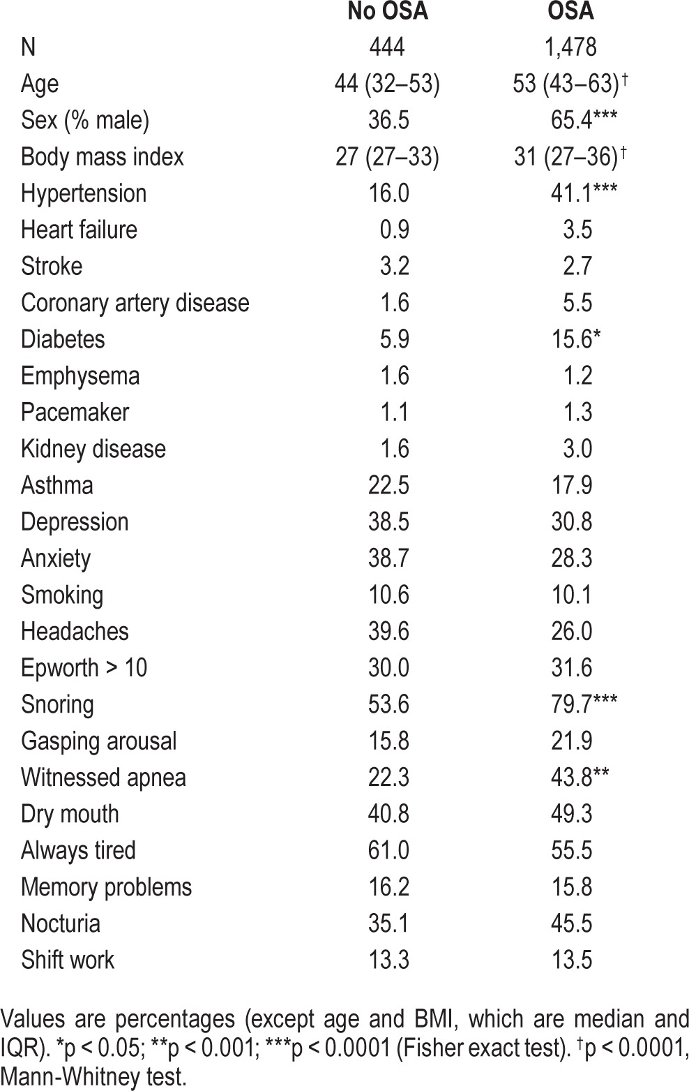
The Partners Institutional Review Board approved analyses of our clinical sleep laboratory database without requiring additional consent for use of this routinely acquired self-reported and objective data. The MGH sleep lab uses the GRASS recording system and follows AASM practice standards, including regular scoring evaluation of technologists compared to the medical director as gold standard. All scoring technologists are certified. Inclusion criteria were: age ≥ 18 years, and underwent clinical polysomnography (PSG) in our sleep center between January 2009 and June 2013, without regard to clinical reason. This time frame spans the major insurance changes of 2011. Insurance changes likely influenced the population of patients approved for in-lab testing. However, in the current cohort, comorbidities such as heart disease and stroke did not appear overrepresented (< 5%; Table 1).

Table 1.

Cohort characteristics.

The apnea-hypopnea index (AHI) for the diagnostic portion of the split-night studies was higher than that of the diagnostic PSGs, as expected given that diagnostic PSGs included those without OSA, and split-night protocols require moderate or greater OSA. Because of variation in the actual value of the AHI due to body position and REM sleep,¹⁶ and whether a split protocol was performed, we pre-specified OSA to be present whenever either AHI was > 5 or the respiratory disturbance index (RDI) was > 10 (even if AHI was < 5), without further subdividing by severity category, using the diagnostic recordings. The AHI used the 4% rule to define hypopneas. The RDI included apneas, hypopneas, and respiratory event related arousals (defined by EEG scoring per AASM guidelines).

Self-reported data were obtained via a standardized pre-PSG questionnaire administered to all patients undergoing PSG. The questionnaire was used to collect information on comorbidities (stroke, heart failure, diabetes, high blood pressure, etc.) as well as self-reported symptoms of various sleep disorders, including OSA via check-box options. This questionnaire was not initially designed as a screening test, but rather to supply clinical information relevant to technologists and interpreting physicians. The language is intentionally straightforward in this respect. Although it has not undergone independent validation against existing OSA instruments, it does include queries about witnessed apneas, sleepiness and snoring (although not the intensity or frequency, as are included to different degrees in the Berlin Questionnaire and the STOP-BANG). The Berlin Questionnaire and STOP-BANG also query obesity and hypertension, similar to our intake forms.

We allowed all symptoms to be included in the model, beyond those for OSA, such as insomnia, motor restlessness, caffeine intake, and naps. We excluded those with missing questionnaires (although partially completed forms were allowed). Most patients referred to our center are referred for suspected OSA, and ∼75% are referred by non-sleep specialists. We included diagnostic and split-night studies, but not full-night titration studies. The final cohort included 1,922 patients (n = 504 split night).

Data Processing

For each patient, we used the information that we collected to encode d = 32 binary features x_i,1,x_i,2…,x_i,d, as well as a binary outcome y_i. We set the outcome for patient i as y_i = 1 if the patient had OSA, and y_i = −1 otherwise. We produced models using: (i) all features; (ii) a subset of 17 features based on information that could in principle extracted from an electronic medical record (“extractable”); and (iii) a subset of 14 features based on sleep-related information that requires sleep-specific clinical queries (“symptoms”). We provide a description of all features and their inclusion in different subsets in Table S1, supplemental material.

Overview of Supersparse Linear Integer Models

A Supersparse Linear Integer Model (SLIM) is a new machine learning method for creating medical scoring systems.¹⁵ Scoring systems are linear classification models that require users to add, subtract, and multiply a few small integers to make a prediction. These models are widely used in medical applications because they allow clinicians to make quick predictions by hand, without the use of a calculator or computer (see, e.g., the CHADS₂ scoring system for predicting stroke in atrial fibrillation,¹⁷ which is widely used but was not created by a machine learning algorithm such as SLIM).

SLIM produces classification models of the form:

Here, x_i,1,x_i,2…,x_i,d are the values of the d features for patient i and ŷ_i represents the predicted class of patient i (e.g. = +1 if patient has OSA). The coefficients λ₁,λ₂,…,λ_d are restricted to small integer values in order to represent the “points” for features 1,…,d. Thus, the model can be seen as a scoring system where the sum λ₁x_i,1 + λ₂x_i,2,…,λ_dx_i,d is the “total score” for patient i and λ₀ is the “threshold score” that has to be surpassed to predict ŷ_i = +1.

SLIM can create simple models that are usually more accurate and sparse in comparison to state-of-the-art machine learning methods because it directly optimizes accuracy and sparsity, without making approximations to reduce computation. Avoiding approximations means that creating (“training”) SLIM models often requires more computation than current methods (minutes or hours depending on the size of the dataset). However, this also allows SLIM to directly produce models that accommodate multiple operational constraints (e.g., SLIM can produce models that obey explicit constraints on the number of features, or the false positive rate, without post-processing or parameter tuning).

Model Training and Validation

We considered two classes of SLIM models: (i) a simple class (“size 5”), with at most 5 features, where each coefficient was restricted to be an integer between −10 and 10, and the score threshold was restricted to be an integer between −100 and 100; (ii) a slightly more complex class (“size 10”), with at most 10 features, where each coefficient was restricted to be an integer between −20 and 20, and the score threshold was restricted to be an integer between −200 and 200. In both classes, we constrained the signs of coefficients for certain features to positive or negative values to ensure that the models would align with existing domain knowledge (Table S1). We trained a “size 5” and “size 10” SLIM model at 19 different points on the ROC curve. Specifically, for each model class, we ran SLIM to produce a model that had the highest true positive rate (TPR) subject to a constraint on the maximum allowable false positive rate (FPR) ≤ 5%, 10%, and so on.

For purposes of validation, we also produced models using 7 other classification methods, namely: (1) L₁-penalized logistic regression (Lasso); (2) L₂-penalized logistic regression (Ridge); (3) L₁ and L₂-penalized logistic regression (Elastic Net); (4) C5.0 decision trees (C5.0T); (5) C5.0 rule lists (C5.0R); (6) support vector machines with a radial basis kernel (SVM RBF); and (7) support vector machines with a linear kernel (SVM Linear).^18–20 Using these methods, we produced classification models at 39 different points of the ROC curve by running the methods with 39 unique combinations of misclassification costs for false positives and false negatives.

For each method, at each of point of the ROC curve (19 points for SLIM with class [i] and class [ii] and 39 points for the other methods), we trained and evaluated 10 models using 10 fold cross-validation, where each of the 10 folds was used in turn as the test fold. To allow for principled comparisons of predictive accuracy between methods and feature sets, we used the same cross-validation folds for each method and for different subsets of the features. In addition, we trained a final SLIM model using all of the data at each point along the ROC curve for use in practice. We produced this model using all of the data, and estimated its true TPR/FPR through mean 10-CV testing TPR/FPR.

We solved all optimization problems for SLIM using the IBM CPLEX 12.6 API, which we accessed through MATLAB 2014b. We limited training time to 1 h per instance of SLIM (time was only a concern for training models using all features: < 10 min was required for training models with the symptom features or the extractable features). We trained models for all other methods using publicly available packages in R 3.1.1 (glmnet, e1071, c50).

RESULTS

Table 1 shows the basic demographics and sleep apnea metrics for the cohort, which included 444 (23%) subjects without OSA (AHI < 5, RDI < 10), and 1,478 (77%) subjects with OSA (of whom n = 1,259 met criteria via AHI > 5, and n = 219 met criteria based on RDI > 10 even if AHI was < 5; similar data were obtained if the latter group was not included in the definition of OSA). Here and throughout, OSA therefore refers to the inclusive definition: AHI > 5 or RDI > 10. The group with OSA had more males, higher BMI, and had a greater proportion reporting hypertension, diabetes, snoring, and witnessed apneas (Table 1).

Figure 1 illustrates the ROC curve comparing the performance of SLIM models from the “size 10” class that were trained using: (i) all features; (ii) features from the “extractable” subset; or (iii) features from the “symptom” subset. We achieved similar performance using all features and extractable features but much poorer performance using only the symptom features. The mean 10-fold cross validation (10-CV) AUC was 0.785 for all features; 0.775 for extractable features (p > 0.5, extractable versus all features), and 0.670 for symptom features (p < 0.0001, symptom versus all features, and versus extractable features). In fact, the performance of models using only extractable features sometimes exceeds the performance of models using all features at some points of the ROC curve, possibly since using a smaller set of features prevents over-fitting.

Figure 1. Receiver operating characteristic curves.

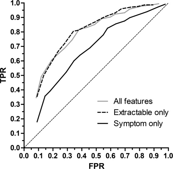
The mean values for 10-fold cross validation (10-CV) true positive rate (TPR; sensitivity) and false positive rate (FPR; 1-specificity) are shown for models that were trained with all features (gray), the subset of “extractable” features (dashed), or the subset of “symptom” features (solid). The diagonal dotted line is the reference for chance performance. Student's t-test revealed p < 0.0001 comparing the symptom feature model with either the extractable model or the full feature set; the full set did not differ from the extractable set (p > 0.5).

As a comparison, we also assessed the performance of models from other state-of-the-art machine learning methods using the same three subsets of features (Table S2, supplemental material). Results of this comparison demonstrate that the predictive utility of extractable features was superior to that of symptom based features, regardless of the classification method used. For instance, the mean 10-CV AUC obtained by Ridge regression is 0.804 for all features, 0.785 for extractable features, and 0.692 for symptom features (note that the AUC is slightly higher than SLIM because Ridge regression does include constraints on the number of coefficients or the signs of coefficients).

To use predictive models as decision tools, we must choose specific cutoff points that balance sensitivity and specificity. Figure 2 shows the performance specifically when the false positive rate (FPR) is constrained to be no more than 20% (yielding a performance that emphasizes specificity at the expense of sensitivity), and separately, when the FPR constraint is loosened to 40% (yielding a performance that emphasizes sensitivity at the expense of specificity). Additional details are shown in Table S3, supplemental material.

Figure 2. Performance accuracy of SLIM models.

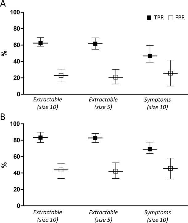
SLIM performance is shown when the models are constrained to a false positive rate (FPR) of either 20% (A) or 40% (B). The true positive rate (TPR) and solid squares, and the FPR (open squares) are given for extractable models of size 5 or size 10, or symptom based features (size 10), as shown on the X axis. The upper and lower 95% confidence intervals are given as error bars in each case. The legend in panel A applies to panel B as well.

A key advantage of SLIM models is their high degree of practicality and interpretability. In Figure 2, we compared SLIM models from the “size 5” and “size 10” class with extractable features at FPR targets of 20% and 40%. The features and their coefficients are shown in Table 2. To demonstrate how these models could be used within a clinical setting, we present SLIM scoring systems for “size 5” and “size 10” for an FPR target of 20% in Tables 3 and 4.

Table 2.

Prediction based on extractable features.

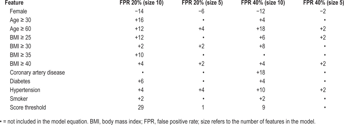
Table 3.

SLIM scoring system (size 10, extractable features, FPR goal of 20%).

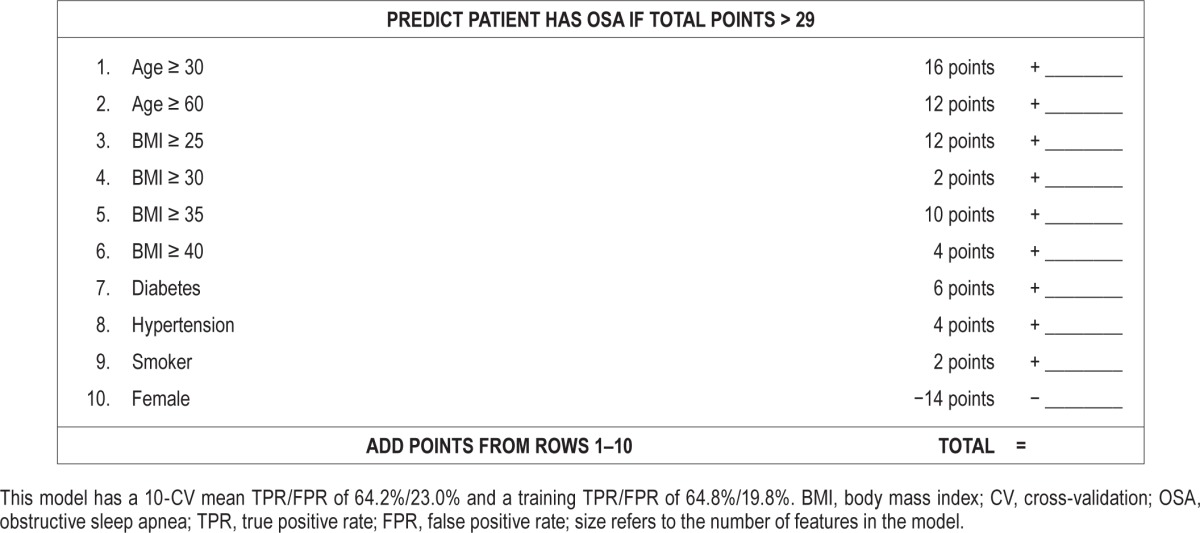
Table 4.

SLIM scoring system (size 5, extractable features, FPR goal of 20%).

As shown, the features selected in the final SLIM models are all associated with an integer coefficient that represents the number of “points” in the final score. Integer coefficients allow clinicians to make quick predictions by hand by tallying the number of points for different features and comparing it to the score threshold. Integer coefficients also provide a high degree of interpretability by helping users gauge the influence of one feature with respect to the others, and allowing them to see how joint values of the features affect the predictive outcome. To see this principle in action, consider the “size 5” SLIM model at FPR 20% in Table 4. This can be interpreted as a rule-based model that says: “if the patient is male, predict OSA if BMI ≥ 30 OR age ≥ 60 OR hypertension; if the patient is female, predict OSA if BMI ≥ 40 AND (age ≥ 60 OR hypertension).”

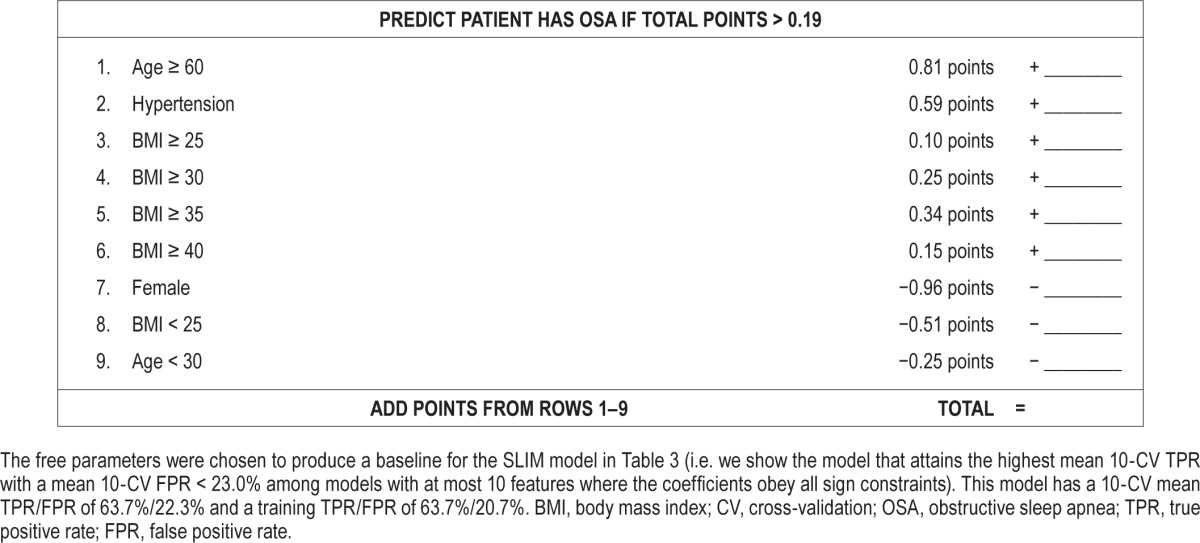
For comparison, in Table 5, we present a scoring system derived from a Lasso model. Specifically, we show the model that attains the highest mean 10-CV TPR among models with mean 10-CV FPR < 23.0%, at most 10 features, and whose coefficients obey all sign constraints (i.e., the same constraints as the SLIM model in Tables 3 and 4). Here, Lasso produces a transparent model that attains similar levels of sensitivity and specificity to the SLIM models in Tables 3 and 4. However, it cannot be used as a scoring system without rounding (which would affect the sensitivity and specificity of the tool). Even if we rounded to one or two digits, the rounded coefficients could not be easily related to illustrate how joint values of the features affect the predictive outcome (as we are able to do for the “size 5” SLIM model discussed in the previous paragraph).

Table 5.

Score function and scoring system derived from a Lasso model.

DISCUSSION

In this study, we used a new machine learning method (SLIM) to create accurate, practical and interpretable tools for predicting the presence of OSA based on a sleep-lab referred population. The SLIM model we created using extractable features has sensitivity (64.2%) and specificity (77%) and likelihood ratio (LR) values (LR⁺, 2.8; LR^-, 0.46) that are within the range of other tools. For example, the STOP-Bang tool yields a sensitivity and specificity for OSA (defined by AHI > 5) of 83.6% and 56.4%, respectively, which yields a positive likelihood ratio (LR⁺) value of 1.9, and a negative likelihood ratio (LR^-) value of 0.29.²¹ Of note, the STOP portion of the STOP-BANG tool, which uses three symptom-based queries, has lower accuracy than the full 8-point STOP-BANG tool, which also includes age, sex, BMI, and neck circumference. The SLIM screening tools also performed similarly to tools produced with other state-of-the-art machine learning methods. The current findings demonstrate that we can create accurate predictive models using features that are in principle extractable from electronic health records—that is, without inquiring specifically as to symptoms associated with OSA. This finding confirms prior literature suggesting that symptom reports carry only modest predictive utility,¹³ and raises the possibility of large-scale OSA screening using data that are routinely available in the electronic medical record.

Clinical Implications

OSA has been associated with important health and wellness concerns ranging from cardiovascular and cerebrovascular morbidity, to metabolic and neuropsychiatric health.^3,22,23 The associations are most evident in those with moderate or severe OSA, while greater uncertainty exists regarding those with mild OSA.^24–29 Improving the accuracy of screening tools is important to address underdiagnosis. Despite the data suggesting that symptom-severity dissociation is prominent in OSA patients, there remains an emphasis on symptoms in screening tools. For example, the tool used by the ARES home apnea test kit for OSA screening assigns much more weight (up to 4-fold) for self-reported snoring, gasping, or witnessed apneas than for self-reporting sleep apnea from a list of medical conditions for which the patient is being treated.³⁰

An alternative approach to screening is to capitalize on the predictive power of medical comorbidities. An important advantage of this approach is that it relies on a method of data gathering that readily lends itself to large-scale implementation. Symptom reporting can be done by patients filling out paper or e-forms, as is done in many sleep labs (including the one in this study). Demographic and medical information, including medications, can in principle be extracted from the electronic medical record automatically, especially as more advanced versions of these systems increasingly allow such extraction. In this way, automated “flags” become a potential implementation that could prompt a clinical action without the need to burden patients or providers with additional forms during a given visit.

Interpreting Performance of Screening Tool Results: Bayes' Theorem

The performance of any screening tool depends on a patient's pretest probability, in addition to the tool's sensitivity and specificity. These three elements are related to one another through Bayes' theorem. As with any screening tool, if a test is applied in a low-prevalence setting, the risk of false positives (i.e., low positive predictive value) will be proportional to how low the prevalence actually is. Likewise, if the test is applied in a high prevalence setting, the risk of false negatives (i.e., low negative predictive value) will be proportional to how high the prevalence actually is. Accordingly, the sensitivity and specificity of a screening tool may change according to the population of patients. In particular, sensitivity will change according to factors such as disease severity, and specificity will change according to characteristics of individuals included in “control” populations.

To illustrate, consider a case where the baseline prevalence of OSA is 10%. In this setting, if the “size 10” SLIM model with extractable features (Table S3) predicted that a patient has OSA, then the posttest probability of the patient having OSA would increase from 10% to 23%. This might then be interpreted as sufficient to engage in further investigation. Similarly, if the “size 10” SLIM model predicted that a patient did not have OSA, then the posttest probability of the patient having OSA would decrease from 10% to 5%. By comparison, the STOP-BANG tool would yield a posttest OSA probability of 17% if positive, and 3% if negative. In a population with high prevalence of, say 70%, a negative result from the “size 10” SLIM model with extractable features would lower the patient's posttest OSA probability to 52% arguably not sufficient to have ruled out OSA.

Limitations

Our study has several limitations that are amenable to future investigation. First, the retrospective cohort consisted of unselected patients referred to a tertiary specialty facility. Although we cannot determine if the results generalize to other settings, with increasing access to clinical databases, the SLIM method could be applied in other settings, potentially identifying population-specific differences in the resulting predictive models, and thus evaluate external validity. Second, the extractable features were not validated with a gold standard; doing so, either by billing codes or natural language text processing, would be expected to improve performance, as there are no doubt false positive and false negative individuals for each of the medical comorbidities we studied. Third, we did not measure the severity of the comorbidities, which might play an important role, as has been shown regarding the severity of hypertension.¹⁴ Despite these limitations, the potential benefits of automated risk assessments based on electronic records using the SLIM method could prove beneficial for addressing the OSA under-diagnosis problem.

In terms of external validity, we note that while the STOP-Bang initial validation in an outpatient surgical population reported sensitivity and specificity for AHI > 5 of 84% and 56%, respectively, more recent evaluations showed less robust values. For example, Boynton et al. tested the STOP-BANG in a population referred for suspected OSA and found sensitivity and specificity of 82% and 48%, respectively, for AHI > 5.³¹ Pataka et al. reported, in a population referred to a sleep clinic, a sensitivity and specificity of 96% and 14%, respectively, for AHI > 5; for the Berlin Questionnaire, sensitivity and specificity were 84% and 35%, respectively.³²

Statistical Discussion

Our results illustrate two important statistical principles: (1) that it is possible that many state-of-the-art machine learning methods produce models that attain roughly the same performance across the full ROC curve (this “multiplicity of good models” is typically referred to as the “Rashomon effect”)³³; (2) that among the set of good models, there may exist simple models that attain just as good, if not better, performance than complex models (typically referred to as “Occam's Razor”).³³

Our results also highlight a different advantage of using simple transparent models, which is that they tend to generalize well out of sample (note, for instance, that the mean 10-CV TPR/FPR is very close to the training TPR/FPR for the SLIM models in Tables 4 and 5). Good generalization is especially important in medical applications. Poor generalization often occurs when a dataset is too small relative to the complexity of the model class. In many medical applications, datasets are underpowered to accurately determine complex models and are at increased risk for over-fitting—this means that they may not maintain the same degree of predictive accuracy when used in practice.

CONCLUSION

The SLIM screening tools attain state-of-the-art performance while maintaining interpretability of the predictive model. These tools can be utilized quickly and easily at the point of care, or could in principle be applied in an automated manner to an electronic medical record database for large-scale OSA screening.

DISCLOSURE STATEMENT

This was not an industry supported study. Dr. Bianchi is co-inventor on pending patent related to a sleep monitoring device, has consulting agreements with GrandRounds, is on the Advisory Board of Foramis, has received travel funds from Servier, and provides expert witness testimony. Dr. Bianchi has received support from the department of Neurology, Massachusetts General Hospital, the Young Clinician Award from the Center for Integration of Medicine and Innovative Technology, the Harvard Catalyst KL2 Medical Research Investigator Fellowship, the Milton Foundation, the Department of Defense, and the MGH-MIT Grand Challenge. Dr. Rudin acknowledges support from Wistron, Siemens, Ford, the MIT Big Data Initiative and the National Science Foundation. Dr. Westover has received support from NIH-NINDS (1K23NS090900-01), and from the Andrew David Heitman Neuroendovascular Research Fund. Mr. Ustun has indicated no financial conflicts of interest.

REFERENCES

- 1.AlGhanim N, Comondore VR, Fleetham J, Marra CA, Ayas NT. The economic impact of obstructive sleep apnea. Lung. 2008;186:7–12. doi: 10.1007/s00408-007-9055-5. [DOI] [PubMed] [Google Scholar]
- 2.Punjabi NM. The epidemiology of adult obstructive sleep apnea. Proc Am Thorac Soc. 2008;5:136–43. doi: 10.1513/pats.200709-155MG. [DOI] [PMC free article] [PubMed] [Google Scholar]
- 3.Kapur VK. Obstructive sleep apnea: diagnosis, epidemiology, and economics. Respir Care. 2010;55:1155–67. [PubMed] [Google Scholar]
- 4.Jennum P, Riha RL. Epidemiology of sleep apnoea/hypopnoea syndrome and sleep-disordered breathing. Eur Respir J. 2009;33:907–14. doi: 10.1183/09031936.00180108. [DOI] [PubMed] [Google Scholar]
- 5.Young T, Skatrud J, Peppard PE. Risk factors for obstructive sleep apnea in adults. JAMA. 2004;291:2013–6. doi: 10.1001/jama.291.16.2013. [DOI] [PubMed] [Google Scholar]
- 6.Collop NA, Tracy SL, Kapur V, et al. Obstructive sleep apnea devices for out-of-center (OOC) testing: technology evaluation. J Clin Sleep Med. 2011;7:531–48. doi: 10.5664/JCSM.1328. [DOI] [PMC free article] [PubMed] [Google Scholar]
- 7.Collop NA, Anderson WM, Boehlecke B, et al. Clinical guidelines for the use of unattended portable monitors in the diagnosis of obstructive sleep apnea in adult patients. Portable Monitoring Task Force of the American Academy of Sleep Medicine. J Clin Sleep Med. 2007;3:737–47. [PMC free article] [PubMed] [Google Scholar]
- 8.Gottlieb DJ, Whitney CW, Bonekat WH, et al. Relation of sleepiness to respiratory disturbance index: the Sleep Heart Health Study. Am J Respir Crit Care Med. 1999;159:502–7. doi: 10.1164/ajrccm.159.2.9804051. [DOI] [PubMed] [Google Scholar]
- 9.Chervin RD, Aldrich MS. The Epworth Sleepiness Scale may not reflect objective measures of sleepiness or sleep apnea. Neurology. 1999;52:125–31. doi: 10.1212/wnl.52.1.125. [DOI] [PubMed] [Google Scholar]
- 10.Eiseman NA, Westover MB, Mietus JE, Thomas RJ, Bianchi MT. Classification algorithms for predicting sleepiness and sleep apnea severity. J Sleep Res. 2012;21:101–12. doi: 10.1111/j.1365-2869.2011.00935.x. [DOI] [PMC free article] [PubMed] [Google Scholar]
- 11.Abrishami A, Khajehdehi A, Chung F. A systematic review of screening questionnaires for obstructive sleep apnea. Can J Anaesth. 2010;57:423–38. doi: 10.1007/s12630-010-9280-x. [DOI] [PubMed] [Google Scholar]
- 12.Bianchi MT. Screening for obstructive sleep apnea: Bayes weighs in. Open Sleep J. 2009;2:56–9. [Google Scholar]
- 13.Skomro RP, Kryger MH. Clinical presentations of obstructive sleep apnea syndrome. Prog Cardiovasc Dis. 1999;41:331–40. doi: 10.1053/pcad.1999.0410331. [DOI] [PubMed] [Google Scholar]
- 14.Logan AG, Perlikowski SM, Mente A, et al. High prevalence of unrecognized sleep apnoea in drug-resistant hypertension. J Hypertens. 2001;19:2271–7. doi: 10.1097/00004872-200112000-00022. [DOI] [PubMed] [Google Scholar]
- 15.Ustun B, Rudin C. Supersparse Linear Integer Models for Optimized Medical Scoring Systems. arXiv. 2015 Available at http://arxiv.org/abs/1502.04269. [Google Scholar]
- 16.Eiseman NA, Westover MB, Ellenbogen JM, Bianchi MT. The impact of body posture and sleep stages on sleep apnea severity in adults. J Clin Sleep Med. 2012;8:655–66. doi: 10.5664/jcsm.2258. [DOI] [PMC free article] [PubMed] [Google Scholar]
- 17.Naccarelli GV, Panaccio MP, Cummins G, Tu N. CHADS2 and CHA2DS2-VASc risk factors to predict first cardiovascular hospitalization among atrial fibrillation/atrial flutter patients. Am J Cardiol. 2012;109:1526–33. doi: 10.1016/j.amjcard.2012.01.371. [DOI] [PubMed] [Google Scholar]
- 18.Friedman J, Hastie T, Tibshirani R. Regularization paths for generalized linear models via coordinate descent. J Stat Softw. 2010;33:1–22. [PMC free article] [PubMed] [Google Scholar]
- 19.Kuhn M, Weston S, Coulter N, Quinlan R. C50: C5. 0 decision trees and rule-based models. 2013.
- 20.Meyer D. Support vector machines: the interface to libsvm in package E1071. 2004.
- 21.Chung F, Yegneswaran B, Liao P, et al. STOP questionnaire: a tool to screen patients for obstructive sleep apnea. Anesthesiology. 2008;108:812–21. doi: 10.1097/ALN.0b013e31816d83e4. [DOI] [PubMed] [Google Scholar]
- 22.Budhiraja R, Budhiraja P, Quan SF. Sleep-disordered breathing and cardiovascular disorders. Respir Care. 2010;55:1322–32. [PMC free article] [PubMed] [Google Scholar]
- 23.Somers VK, White DP, Amin R, et al. Sleep apnea and cardiovascular disease: an American Heart Association/American College of Cardiology Foundation Scientific Statement from the American Heart Association Council for High Blood Pressure Research Professional Education Committee, Council on Clinical Cardiology, Stroke Council, and Council On Cardiovascular Nursing. In collaboration with the National Heart, Lung, and Blood Institute National Center on Sleep Disorders Research (National Institutes of Health) Circulation. 2008;118:1080–111. doi: 10.1161/CIRCULATIONAHA.107.189375. [DOI] [PubMed] [Google Scholar]
- 24.Gottlieb DJ, Yenokyan G, Newman AB, et al. Prospective study of obstructive sleep apnea and incident coronary heart disease and heart failure: the Sleep Heart Health Study. Circulation. 2010;122:352–60. doi: 10.1161/CIRCULATIONAHA.109.901801. [DOI] [PMC free article] [PubMed] [Google Scholar]
- 25.Redline S, Yenokyan G, Gottlieb DJ, et al. Obstructive sleep apnea-hypopnea and incident stroke: the sleep heart health study. Am J Respir Crit Care Med. 2010;182:269–77. doi: 10.1164/rccm.200911-1746OC. [DOI] [PMC free article] [PubMed] [Google Scholar]
- 26.Quan SF, Budhiraja R, Batool-Anwar S, et al. Lack of impact of mild obstructive sleep apnea on sleepiness, mood and quality of life. Southwest J Pulm Crit Care. 2014;9:44–56. doi: 10.13175/swjpcc082-14. [DOI] [PMC free article] [PubMed] [Google Scholar]
- 27.Marin JM, Carrizo SJ, Vicente E, Agusti AG. Long-term cardiovascular outcomes in men with obstructive sleep apnoea-hypopnoea with or without treatment with continuous positive airway pressure: an observational study. Lancet. 2005;365:1046–53. doi: 10.1016/S0140-6736(05)71141-7. [DOI] [PubMed] [Google Scholar]
- 28.Punjabi NM, Caffo BS, Goodwin JL, et al. Sleep-disordered breathing and mortality: a prospective cohort study. PLoS Med. 2009;6:e1000132. doi: 10.1371/journal.pmed.1000132. [DOI] [PMC free article] [PubMed] [Google Scholar]
- 29.Peppard PE, Young T, Palta M, Skatrud J. Prospective study of the association between sleep-disordered breathing and hypertension. N Engl J Med. 2000;342:1378–84. doi: 10.1056/NEJM200005113421901. [DOI] [PubMed] [Google Scholar]
- 30.Levendowski D, Olmstead R, Popovic D, Carper DL, Berka C, Westbrook P. Assessment of obstructive sleep apnea risk and severity in truck drivers: validation of a screening questionnaire. Sleep Diagn Ther. 2007;2:20–6. [Google Scholar]
- 31.Boynton G, Vahabzadeh A, Hammoud S, Ruzicka DL, Chervin RD. Validation of the STOP-BANG Questionnaire among patients referred for suspected obstructive sleep apnea. J Sleep Disord Treat Care. 2013;2(4) doi: 10.4172/2325-9639.1000121. [DOI] [PMC free article] [PubMed] [Google Scholar]
- 32.Pataka A, Daskalopoulou E, Kalamaras G, Fekete Passa K, Argyropoulou P. Evaluation of five different questionnaires for assessing sleep apnea syndrome in a sleep clinic. Sleep Med. 2014;15:776–81. doi: 10.1016/j.sleep.2014.03.012. [DOI] [PubMed] [Google Scholar]
- 33.Breiman L. Statistical modeling: the two cultures (with comments and a rejoinder by the author) Stat Sci. 2001;16:199–231. [Google Scholar]
Associated Data
This section collects any data citations, data availability statements, or supplementary materials included in this article.