SVD Compression for Magnetic Resonance Fingerprinting in the Time Domain

Abstract

Magnetic resonance fingerprinting is a technique for acquiring and processing MR data that simultaneously provides quantitative maps of different tissue parameters through a pattern recognition algorithm. A predefined dictionary models the possible signal evolutions simulated using the Bloch equations with different combinations of various MR parameters and pattern recognition is completed by computing the inner product between the observed signal and each of the predicted signals within the dictionary. Though this matching algorithm has been shown to accurately predict the MR parameters of interest, one desires a more efficient method to obtain the quantitative images. We propose to compress the dictionary using the singular value decomposition (SVD), which will provide a low-rank approximation. By compressing the size of the dictionary in the time domain, we are able to speed up the pattern recognition algorithm, by a factor of between 3.4-4.8, without sacrificing the high signal-to-noise ratio of the original scheme presented previously.

I. Introduction

Magnetic resonance fingerprinting (MRF) [1] is a relatively new technique in the field of MR and one of its major contributions is to simultaneously provide quantitative maps of multiple tissue parameters via a novel data acquisition. At the heart of this quantitative mapping is a dictionary composed of simulated signal evolutions calculated using the Bloch equations with different combinations of the MR parameters of interest, such as T₁, T₂, and off-resonance. In the original implementation, the observed signal evolutions were matched to distinct dictionary entries using template matching, where the inner product was computed between an observed signal and each of the dictionary entries to find the maximum, thus retrieving the parameter combinations unique to that entry. While it was shown in [1] that this procedure is robust and can accurately predict the parameter values, it is desirable to reduce the number of computations needed while maintaining accuracy.

The singular value decomposition (SVD) [2] of a matrix is a useful tool that can provide information about the properties of a matrix and can be applied to a variety of problems, including the solution of linear least squares problems [3] and dimensionality reduction through principal component analysis (PCA) [4], [5]. Data compression using the SVD has been extensively studied, for example in the compression of ECG signals [6] and for images [7], [8]. The SVD has also been used to create digital watermarks for copyright protection [9], [10]. In the field of text mining, the SVD is applied to the term document matrix in a process known as latent semantic indexing [11], [12] to reveal the intrinsic structure of the matrix and to reduce its size. The SVD has been applied to transform gene expression data into “eigengenes” and “eigenarrays” [13] and also to model the distribution of yeast mRNA gene lengths [14]. Keeping in mind the close connection between the eigenvalue decomposition and the SVD, facial recognition is yet another area where matrix factorization plays a pivotal role in data compression and pattern recognition [15].

SVD encoded MR was introduced and implemented in [16], [17] to reduce acquisition time through dynamically adaptive imaging, though it has been argued [18], [19] that other methods for dynamic MRI are more suitable due to the tendency of SVD methods to reproduce features from the reference image. The SVD has also been considered to modify the block uniform resampling (BURS) algorithm for gridding nonuniform k-space data [20]. More recently, both the SVD and eigenvalue decomposition have been used in parallel MRI as a way to calculate coil sensitivity maps, establishing a clear link between SENSE and GRAPPA [21], [22], and the SVD has also been used on low-tip-angle gradient-echo images to calculate the $B_1^{+}$ and $B_1^{-}$ fields [23].

The goal of this paper is to apply the SVD to the MRF dictionary to reduce its size in the time domain, resulting in faster reconstruction of the tissue parameters without sacrificing the accuracy of this process, already demonstrated in [1].

II. Quantitative Imaging from MRF

One of the main contributions of MRF to the field of magnetic resonance imaging is its ability to efficiently and simultaneously produce quantitative images of tissue parameters. Rather than assuming an exponential signal evolution model, in [1] a pseudorandom acquisition scheme is considered, where parameters such as repetition time, flip angle, and sampling pattern are varied randomly to create spatial and temporal incoherence between signals coming from different materials. The random nature of the acquisition scheme allows for specific tissues to exhibit unique signal evolutions, or fingerprints, that can identify each to its inherent MR parameters. In the initial implementation, a dictionary is calculated by solving the Bloch equations to simulate signal evolutions as functions of different combinations of T₁ and T₂ relaxation times and off-resonance frequencies. Given the large range of these parameters that one might expect to see in vivo, the dictionary is a comprehensive database of these fingerprints, which will allow for an accurate mapping of the MR parameters.

In the original work presented in [1], an inversion recovery balanced steady state free-precession (bSSFP) sequence was used, and as this type of sequence is known to be sensitive to T₁, T₂, and off-resonance [24], these parameters were used in the calculation of the dictionary. Recently, an inversion recovery FISP-based sequence was also used to quantify T₁ and T₂ in the MRF framework [25]. We consider both sequences in this work.

Denote the dictionary by D ∈ ℂ^n×t where n is the number of parameter combinations and t is the number of time points. Denote by d_j, j = 1,…, n the jth row of D, or the jth dictionary entry. As described in [1], for an observed signal evolution, its dictionary match is determined by a process similar to query or template matching: the observed signal evolution, denoted x, is compared to each dictionary entry by using the complex inner product to determine which entry it matches with highest probability, thereby assigning to it the values for T₁, T₂ and off-resonance unique to that entry. The dictionary entry d_ℝ is chosen that satisfies

$$d_{\ell }=\text{arg}\underset{\begin{array}{c}\hfill d_j,\hfill \\ \hfill j=1,\dots ,n\hfill \end{array}}{\text{max}}\mid d_j{x}^{\ast }\mid ,$$ (1)

where x^∗ denotes the conjugate transpose of the vector x and | · | represents the modulus. The dictionary entries and measured signal evolutions are normalized to have unit length, i.e., ∥x∥ = ∥d_j∥ = 1, j = 1, …, n, with ∥ · ∥ denoting the usual Euclidean norm. Once we have recovered the match, the signal is assigned the values for the parameters T₁, T₂, and off-resonance corresponding to the matching entry.

III. SVD background

Every matrix A ∈ ℂ^p×q can be written using the SVD [2], which is given by

$$A=U\Sigma V^{\ast },$$

where U ∈ ℂ^p×p and V ∈ ℂ^q×q are unitary matrices, and Σ ∈ ℝ^p×q is a diagonal matrix containing the nonincreasing singular values σ_i, i = 1,…, min{p, q}. The columns of U, denoted u₁,…, u_p are called the left singular vectors, and similarly, the columns of V, denoted v₁,…, v_q are called the right singular vectors.

A rank-k approximation of A is given by a truncated sum of rank-one matrices, written as

$$A^{\left(k\right)}=\sum _{i=1}^k{\sigma }_i{u}_i{v}_i^{\ast },$$ (2)

and it can be shown [26] that this is the “best” low-rank approximation of A, that is,

$$\parallel A^{\left(k\right)}-A{\parallel }_2=\text{inf}\parallel B-A{\parallel }_2$$

where the infimum is taken over all p × q matrices B with rank less than or equal to k.

The total energy of A is defined to be the sum of the squares of its singular values,

$$E=\sum _{i=1}^r{\sigma }_i^2,$$ (3)

and the energy ratio [6] represents the fraction of the energy retained in the rank-k approximation A ^(k),

$$e\left(k\right)=\frac{1}{E}\sum _{i=1}^k{\sigma }_i^2.$$ (4)

The energy ratio can be useful in determining an appropriate truncation index for a low-rank approximation that retains as much of the information from the original matrix as desired.

IV. Methodology

We will use a pattern recognition algorithm similar to the eigenface method presented by Turk and Pentland in [15], in which facial recognition is performed using the projection of images onto the lower dimensional subspace spanned by the eigenvectors corresponding to the largest eigenvalues.

We apply the SVD to the MRF dictionary, writing

$$D=U\Sigma V^{\ast },$$ (5)

where U, V, and Σ are as described in the previous section. Let r = rank(D) and note that in this article, we assume that n > t.

For a given index k, 1 ≤ k ≤ r, the truncated SVD (2) can be written in matrix form, yielding the low-rank approximation of the dictionary,

$$D\approx U_k{\Sigma }_k{V}_k^{\ast },$$

where U_k = [u₁,…, u_k] denotes the matrix containing the first k left singular vectors and similarly for Σ_k, V_k.

Another property of the SVD is that the first r right singular vectors {v₁,…, v_r } form an orthonormal basis for the rows of D, that is, each dictionary entry can be written as a linear combination of these orthogonal vectors. By projecting the dictionary onto the subspace spanned by the first k singular vectors {v₁,…, v_k }, we have a representation of the dictionary in the lower-dimensional space ℂ^k, by multiplying

$$D_k=D{V}_k.$$

We will call this lower dimensional space the “SVD space” for simplicity.

A. Template Matching in the SVD space

An observed MR signal x is projected onto the same subspace spanned by the vectors in V_k by multiplying

$$x_k=x{V}_k,$$

and now the template match in equation (1) can be computed in the SVD space. We search for the dictionary entry so that

$$\begin{array}{cc}\hfill d_{\ell }& =\text{arg}\underset{\begin{array}{c}\hfill d_j,\hfill \\ \hfill j=1,\dots ,n\hfill \end{array}}{\text{max}}\mid \left(d_j{V}_k\right)x_k^{\ast }\mid \hfill \\ \hfill & =\text{arg}\underset{\begin{array}{c}\hfill d_j,\hfill \\ \hfill j=1,\dots ,n\hfill \end{array}}{\text{max}}\mid \left(d_j{V}_k\right){\left(x{V}_k\right)}^{\ast }\mid \hfill \\ \hfill & =\text{arg}\underset{\begin{array}{c}\hfill d_j,\hfill \\ \hfill j=1,\dots ,n\hfill \end{array}}{\text{max}}\mid d_j{V}_k{V}_k^{\ast }{x}^{\ast }\mid .\hfill \end{array}$$

Note that since V is a unitary matrix, the product V_k V_k^∗ will approach the identity matrix as the truncation index k increases, thus approaching the original template matching scheme (1). We outline the steps for template matching in the SVD space in Algorithm 1.

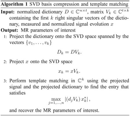
Though there is the added step of projecting the observed signals onto the SVD space, the number of computations required in the template match will be reduced, thereby reducing the amount of time required to compute the parameters. The signal is first projected, requiring ~ 2kt complex operations, and then the inner product is computed in ℂ^k, requiring ~ 2nk complex operations for ~ 2k(n + t) total complex operations. Comparing this with the ~ 2nt complex operations required per pixel for the inner product in the full template match, the number of computations can be significantly reduced depending on the choice of k. Note that in both the SVD and full template matches, the result of computing the inner product in step 3 of the algorithm is an n × 1 vector giving the uncentered correlation between the signal and each dictionary entry. The final step in both is to compute the modulus of each entry from this vector and locate the maximum. We use the operation count as an indication that the SVD method will result in decreased computation time, though due to discrepancies in implementations, memory requirements, etc., we do not expect operation count to translate linearly to computation time.

B. Projecting the k-space data

Alternatively, instead of projecting the data after image reconstruction as in step (2) of Algorithm 1, we can project the raw k-space data prior to gridding the nonuniform spiral data and applying the inverse Fourier transform [27] to obtain equivalent results. The general idea of our proposed method is shown in Fig. 1. On the top is the procedure as outlined in Algorithm 1, in which the raw data are undersampled in k-space as in [1] and then gridding and image reconstruction are performed at each time point to produce t images corrupted with significant errors as a result of the undersampling. Taking advantage of the fact that the Fourier transform is linear, it is possible to switch the order of operations and project the undersampled k-space data before performing gridding and image reconstruction, without significantly changing the resulting parameter maps. Using the SVD, the information from the dictionary simulated over t points is condensed down to k < t points, and as a result, k images are reconstructed. The resulting images are called the singular images. This schematic is shown on the bottom of Fig. 1. Errors between parameter maps computed with the SVD applied before and after image reconstruction are noted in less than 1% of pixels.

Fig. 1.

On the top is a schematic of the current MRF image reconstruction step followed by a projection onto SVD space and template matching. Data are undersampled in k-space at each of t time points and then reconstructed to produce images that are corrupted with significant errors due to the undersampling. On the bottom is a schematic of projecting the raw k-space data prior to image reconstruction, resulting in the singular images which are then used in template matching in the SVD space.

V. Dictionary Analysis

The dictionary for MRF is simulated by solving the Bloch equations given a particular acquisition sequence while varying the inputs for MR parameters such as T₁ and T₂ relaxation times and off-resonance frequencies. In the present work, we consider MRF dictionaries formed from two different types of sequences, an inversion recovery bSSFP sequence, as is used in [1], and an inversion recovery FISP sequence, used with MRF more recently in [25]. Both sequences are sensitive to T₁ and T₂ relaxation times, though only the bSSFP sequence is sensitive to off-resonance frequencies.

Since the dictionary is precomputed and stored before scanning or data acquisition, the time to compute the dictionary is not a significant factor, allowing for different dictionaries to be used depending on the sequence and application. The step sizes for T₁ and T₂ relaxation times can be varied to modify the dictionary; a smaller step size will allow for greater accuracy and precision in the resulting parameter maps while a larger step size can control the dictionary size. The addition of the off-resonance parameter in the bSSFP sequence means that the relaxation time step sizes will need to be larger to keep the size of the dictionary under control; in Tables I and II, we outline the T₁ and T₂ step sizes and ranges for a bSSFP dictionary and a FISP dictionary that we will use in this work.

TABLE 1.

Step sizes and ranges for T₁ and T₂ in the bSSFP dictionary. All times are in ms.

bSSFP	Range	Step size
T 1	[100, 2000] [2000, 5000]	20 300
T 2	[20, 100] [100, 200] [300, 1900]	5 10 200

TABLE II.

Step sizes and ranges for T₁ and T₂ in the FISP dictionary. All times are in ms.

FISP	Range	Step size
T 1	[20, 3000] [3000, 5000]	20 200
T 2	[10, 300] [300, 500] [500, 900]	5 50 200

All computations and results presented here were performed using Matlab (The MathWorks, Inc.) on a standard desktop computer. Computation of the right singular vectors of a complex dictionary of size 363 624 × 1000 took about 2 and a half minutes using the built in function in Matlab. Please note that this computation needs to be done only once for each dictionary so that this step can be performed without significant time constraints.

A. bSSFP dictionary

We consider first a bSSFP dictionary created for a phantom data set containing n = 363 624 combinations of T₁, T₂, and off-resonance, simulated at each of t = 1000 time points. 3336 different combinations of T₁ and T₂ values are used, with the ranges and step sizes outlined in Table I. 109 different off-resonance frequencies are used, in 1 Hz increments from −50 to 50 Hz and also containing the values −250, −230, −210, −190, 180, 200, 220, and 240 Hz, resulting in a complex matrix of size 363 624 × 1000.

Plotted in Fig. 2, are the singular values of this particular dictionary and the associated energy ratio for the first 200 values, enforcing the idea that most of the information is concentrated in the first 200 singular values and vectors. Table III displays the energy ratio for a selected number of k singular values.

Fig. 2.

The singular values of a bSSFP dictionary of size 363 624 × 1000 (left) and the energy ratio of the first 200 singular values (right). The energy ratio quickly approaches 1.

TABLE III.

Energy ratio of the first k singular values of the bSSFP dictionary of size 363 624 × 1000.

k	10	25	50	100	200
e(k)	0.9422	0.9700	0.9840	0.9939	0.9989

The projection of the observed signal x gives a k-dimensional weight vector x_k = [xv₁, xv₂,…, xv_k ], which can be used to approximate x as a linear combination of the first k right singular vectors, i.e.,

$$x\approx \sum _{i=1}^k\left(x{v}_i\right)v_i.$$

In Fig. 3 are plotted an observed signal evolution gathered from undersampled data compared to its match from the dictionary as found from template matching, and its approximation using k = 200, 100, and 25 singular vectors.

Fig. 3.

Observed signal evolution and its dictionary match from template matching (upper left) and approximations using the basis of the singular vectors in V_k, with k = 200, 100 and 25. Damping of the oscillations in the original signal is observed as fewer singular vectors are used.

Using fewer singular vectors in the approximation has the effect of damping the oscillations in the signal, though there is a trade off between controlling the fluctuations in the signal and maintaining the accuracy of the dictionary match. This kind of filtering effect from excluding the smallest singular values is well known and is discussed, for example, in [28].

To assess the performance of the SVD basis compression and template matching, the signal-to-noise ratio (SNR) of the output is computed as the mean value divided by the standard deviation of the values using various levels of noise. We draw a dictionary entry at random and add to it simulated Gaussian white noise and then perform the SVD basis compression and template match using Algorithm 1 to predict the T₁, T₂ and off-resonance values and compare these with the true values. The process is repeated 1000 times and the SNR is computed; results of output SNR versus input SNR are shown in Figure 4 using 25, 50, 100, and 200 singular vectors. We note that both aliasing due to undersampling and additive noise contribute to the oscillations and fluctuations seen in the observed signal. Though aliasing will dominate the effect of the noise, the sequence was designed using randomized spatial encoding so that the effects of aliasing will mimic high levels of Gaussian noise, hence we only consider Gaussian noise in our SNR simulations. At high levels of simulated Gaussian noise, this can serve as an approximation of the observed noise and aliasing for purposes of the SNR calculation. In the case of off-resonance, the SNR of the full and SVD methods are approximately equal using as few as 100 singular vectors at all levels of input SNR. For T₁ and T₂, 200 singular vectors are more appropriate, implying that the data can be compressed to approximately 20% of the original length and still retain much of the information inherent to the original signal. For each of the parameters, the output SNR tends to increase with higher levels of input SNR, but as fewer singular vectors are used, a reduction in output SNR is seen, indicating that with low levels of noise, using too few singular vectors results in an overdamping of the observed signals.

Fig. 4.

Output versus input SNR of SVD compression combined with template matching for a bSSFP dictionary using 25, 50, 100, and 200 singular vectors, compared with the SNR of the template matching using the full dictionary. On the left is the SNR for T₁, T₂ is in the center, and off-resonance is on the right.

In Fig. 5 are the plots of output SNR versus the energy ratio for each of the three parameters, at a fixed input SNR level of approximately 10, demonstrating that including more singular vectors in the approximation will improve the output SNR of the process.

Fig. 5.

Output SNR plotted as a function of selected values of the energy ratio of the singular vectors for a bSSFP dictionary. The input SNR is chosen to be approximately 10, and the number of singular vectors used ranges from 1 up to 300.

B. FISP dictionary

More recently, MRF has been applied to other types of sequences, including an inversion recovery FISP sequence [25], which displays different sensitivities than the bSSFP sequence from the previous section. Most noticeably, the FISP sequence is not sensitive to off-resonance, so the dictionary is constructed using only combinations of T₁ and T₂ relaxation times, allowing for a finer dictionary with smaller time steps.

We consider here a dictionary containing n = 10 169 combinations of T₁ and T₂; see Table II. The dictionary is simulated over t = 1500 time points, resulting in a matrix of size 10 169 × 1500.

Removal of the off-resonance parameter allows for a more distinct dictionary structure, which is noticeable in the rapid decay of the singular values, as shown in the left of Fig. 6. Plotted on the right in Fig. 6 are the energy ratios associated with the first 50 singular values, which very quickly reach 1, as shown in Table IV, indicating that the dictionary is highly compressible.

Fig. 6.

Singular values of the FISP MRF dictionary (left) and the energy ratio of the first 50 singular values (right). The dimensions of the dictionary are 10 169 × 1500.

TABLE IV.

Energy ratio associated with the FISP dictionary of dimension 10 169 × 1500.

k	1	2	5	10	25	50
e(k)	0.9023	0.9543	0.9990	1	1	1

Performing a simulation to test the SNR of the FISP dictionary as in the previous section yields similar results, but shows that the FISP dictionary is much more compressible due to the removal of the off-resonance parameter. In Fig. 7, we show the SNR of the FISP dictionary for k = 2, 5, 8, 10 and 25 singular vectors. The SNR of the full template match is achieved with as few as 10 singular vectors, implying that the signal can be compressed to 1 – 2% of its the original length.

Fig. 7.

Output versus input SNR of SVD compression combined with template matching for a FISP dictionary using 2, 5, 8, 10, and 25 singular vectors, compared with the SNR of the full template matching scheme. On the left is the SNR for T₁ and on the right is the SNR for T₂.

VI. Examples

We present examples of the methods discussed in the previous sections using both phantom and in vivo data, using appropriate dictionaries as noted.

A. Phantom Data

We first test Algorithm 1 on undersampled data collected using a phantom with the bSSFP sequence and dictionary described in the Section V-A. Data were collected using the same protocol as in [1] and are highly undersampled using a one-shot spiral trajectory in k-space. The SVD was then applied to the reconstructed images to obtain projections in the SVD space and template matching was performed to retrieve T₁ and T₂ values. A diagram of the phantom is shown in Fig. 8 to indicate one region we will reference later. The resolution of the reconstructed images is 128 × 128 pixels.

Fig. 8.

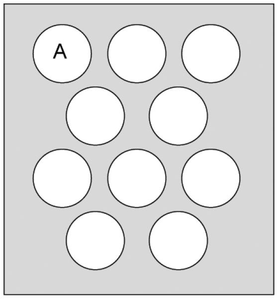
Diagram of the phantom. Region A is indicated, as it is referred to in the text

In Fig. 9, we show the T₁ and T₂ maps computed using the SVD compression and template match with k = 200 singular vectors; comparisons of the SVD computed results with the full template match are shown in Fig. 10. Both the SVD and full methods are consistent in that they predict the same T₁ and T₂ values for this data set. More variations between the two methods are evident as the number of singular vectors used is reduced; see Fig. 11.

Fig. 9.

Parameter maps showing T₁ (left) and T₂ (right) for the phantom data from Section VI-A using k = 200 singular vectors. The units for T₁ and T₂ are in ms.

Fig. 10.

Correlation plots to compare the computed T₁ and T₂ values using the full template match and the SVD template match with 200 singular vectors. Note that the mean values of the two methods are virtually indistinguishable. The error bars represent one standard deviation of the measured data.

Fig. 11.

Correlation plots to compare the computed T₁ and T₂ values using the full template match and the SVD template match with 25 singular vectors. The error bars represent one standard deviation of the measured data.

Assuming that the true T₁ and T₂ values are fairly constant through individual regions within the phantom, we expect the variation of the predicted parameters to be quite small for both methods. This is seen in Figs. 10 and 11 where the error bars represent one standard deviation of the predicted pixel-wise values. In the case of T₁, the error bars are very small except within region A of the phantom; this is likely due to the effect of the highly undersampled spiral data. The mean values of both T₁ and T₂ are virtually indistinguishable for k = 200, and in the case of k = 25, the SVD method appears to predict slightly lower values, particularly for T₂.

In Fig. 12 we display the Bland-Altman plots to compare T₁ and T₂ values computed using the full template match with the SVD method. The horizontal dashed lines show a 95% confidence interval for the difference between the computed and standard values. In the case where k = 200, the SVD results differ from the full template match results in only three pixels for T₁ and two pixels for T₂. In both of these cases, the difference is exactly equal to one step size, suggesting that using a finer dictionary may improve the results. In the case where k = 25, the SVD results differ, though note that the differences between the two methods are within 1–2 steps of the dictionary resolution. Reconstructions of the parameters took just 7.3 seconds using 200 singular vectors in the compression, whereas the full template match took 31 seconds, allowing for a factor of approximately 4 increase in speed for the parameter mapping without loss of accuracy.

Fig. 12.

Bland-Altman plots of the computed SVD using 200 (top) and 25 (bottom) singular vectors compared to the full template match. The dashed lines indicate a 95% confidence interval for the difference between the SVD and full methods. For k = 200, there are only three and two pixels for T₁ and T₂, respectively, that do not match up exactly with the results from the full template match, and these differences are only one step in the dictionary resolution. While there are points that lie outside of the 95% confidence interval for both T₁ and T₂ in the case where k = 25, the differences are small and are within 1 – 2 steps in the dictionary resolution.

Computation times for various values of k are shown in Table V.

TABLE V.

Computation time (in seconds) of the SVD template matching lgorithm for various values of k in the region of interest for the phantom data of Section VI-A using the bSSFP sequence.

k	10	25	50	100	125	150	175	200
time (s)	3.4	3.5	4.1	5.2	5.8	6.3	6.9	7.3

B. Volunteer Data: bSSFP sequence

We apply the SVD method to raw volunteer data, collected on a 1.5 T whole body scanner (Siemens Espree, Siemens Healthcare) using a spiral trajectory with 48 spiral arms.

1) Singular Images

Previously, the data in k-space were reconstructed to obtain a set of 1000 undersampled images each formed from the data collected from one spiral arm; see Fig. 13 for an example of one of these images. By applying the SVD of the dictionary to the raw data, we instead reconstruct k images by combining the data from each of the 48 spiral arms at each of the 1000 time points. The first three of these singular images are shown in Fig. 14. The image resolution is 128 × 128 pixels. We point out that since we do not center the dictionary prior to computing the SVD, the first singular image is a close approximation of the mean [5]. The template matching algorithm is then applied at each pixel location using the sequence of singular images as the SVD compressed signals.

Fig. 13.

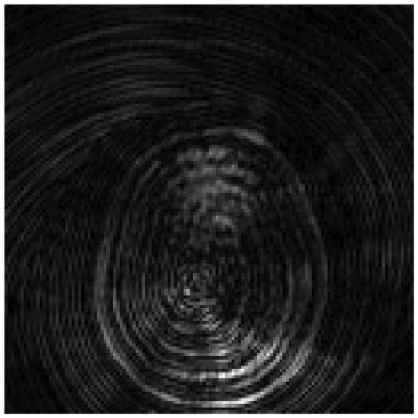
Reconstructed image from undersampled data collected using a one-shot spiral trajectory. This is the 2nd image out of 1000 reconstructions; all have similar spiral artifacts due to the undersampling in k-space.

Fig. 14.

First three singular images.

2) Volunteer Results

After obtaining the compressed signals from the previous section, we perform the template match in the SVD space to produce the quantitative maps for T₁, T₂ and off-resonance. To perform the full template match on the masked image took 167 seconds, whereas the template match in the SVD space took 24 seconds using 25 singular vectors and 49 seconds using 200 singular vectors. In Fig. 15 are plotted the computed parameter maps for k = 200, which was chosen based on the energy ratio of the dictionary singular values.

Fig. 15.

Parameter maps for T₁ (left), T₂ (middle), and off-resonance (right) using k = 200 singular vectors for template matching for the example in Section VI-B with the bSSFP dictionary. The scales for T₁ and T₂ are in ms, the scale for off-resonance is in Hz.

The percent difference maps are computed at each pixel, for example for T₁, by

$$\frac{{T_1}^{\text{SVD}}\left(j\right)-{T_1}^{\text{MRF}}\left(j\right)}{{T_1}^{\text{MRF}}\left(j\right)}\times 100\%$$

where $T_1^{\text{SVD}}\left(j\right)$ denotes the computed T₁ value at pixel j using the SVD method and $T_1^{\text{MRF}}\left(j\right)$ denotes the computed T₁ value at pixel j using the full template match. The percent difference maps are shown in Fig. 16 as compared to the full template match for k = 200 singular vectors, shown on a scale of ±10% for T₁ and T₂, and a scale of ±2% for off-resonance. The mean percent differences over the entire brain are 0.6%, 1.8%, and 1.1% for T₁, T₂ and off-resonance, respectively. These results demonstrate the effectiveness of our algorithm at reducing the computation time while producing good approximations of the parameter maps.

Fig. 16.

Percent differences of the parameter maps shown in Fig. 15 computed using the SVD method as compared to the maps produced using the full template match. On the left is shown the percent difference for T₁, in the middle, T₂, and on the right, off-resonance. The scales for T₁ and T₂ are ±10% and for off-resonance, the scale is ±2%.

C. Volunteer Data: FISP sequence

We next apply the SVD algorithm to a set of data acquired from a volunteer scan on a 1.5 T whole body scanner (Siemens Espree, Siemens Healthcare) using again a spiral trajectory with 48 spiral arms. We use the FISP dictionary as described in Section V-B, and by considering the energy ratios plotted in Fig. 6 and shown in Table IV, we use k = 25 singular vectors for the projection and template matching. The reconstructed images are 256 × 256 pixels. Computation time for the T₁ and T₂ parameter maps was 31.9 seconds for the full template match and 6.6 seconds for the SVD match with 25 singular vectors. Parameter maps for T₁ and T₂ computed using the SVD method are shown in Fig. 17.

Fig. 17.

Parameter maps for T₁ (left) and T₂ (right) using k = 25 singular vectors for template matching with a FISP sequence applied to the example in Section VI-C. The scales for both are in ms.

The percent difference maps are shown in Fig. 18, on a scale of ±5% as compared with the full template match. The mean percent differences over the brain are 0.2% for T₁ and 0.4% for T₂, demonstrating an even closer match of the SVD and full methods using the FISP dictionary as opposed to the original bSSFP sequence, likely due in part to the smaller step sizes used in the dictionary and the exclusion of the off-resonance parameter.

Fig. 18.

Percent differences of the parameter maps shown in Fig. 17 computed using the SVD method with k = 25 singular vectors as compared to the maps produced using the full template match. The percent difference for T₁ is on the left and T₂ on the right. The scales for both are ±5%.

D. Motion Tolerance

An important property of the MRF method that was shown in [1] is motion error tolerance. We use the same data set acquired using a bSSFP sequence in [1], in which the volunteer was instructed to move their head during the last 3 seconds of the 15 second scan. The parameter maps were reconstructed two times, initially using the first 1000 time points of the acquired data that were free of motion, and then by adding on the next 200 time points to obtain a data set that includes both the stationary and motion-corrupted data. The dictionaries and data were projected onto the SVD space using k = 200 singular vectors. Note that the dictionaries between the stationary and motion-corrupted experiments differ only in the number of time points, the first 1000 time points of each are the same.

Results of the stationary and motion-corrupted T₁ and T₂ maps are shown in Fig. 19 with no significant difference seen in the results. The percent difference over the brain between the stationary and motion-corrupted data for T₁ is 0.5% and for T₂ it is 2.7%, indicating that the SVD method is also robust to the motion-corrupted data.

Fig. 19.

T₁ and T₂ maps to demonstrate robustness of the SVD method to motion. Plots (a) and (c) are the T₁ and T₂ maps, respectively, computed using the SVD method with the motion-free data. Plots (b) and (d) are the corresponding T₁ and T₂ maps computed using the SVD method with the motion-corrupted data. 200 singular vectors were used in the SVD template matching.

As before, we compute the percent differences between the parameter maps as computed with the SVD using 200 singular vectors compared to those obtained using the full template match. For the stationary data, the percent difference for T₁ between the two methods is −0.2% and for T₂ it is −0.01%. For the motion corrupted data, the differences between the SVD and full results are similar: −0.2% for T₁ and −0.03% for T₂.

VII. Discussion

The advantage of the SVD template match over the full template match is in the reduced computation time; in the case of the phantom data, the SVD method was about 4 times faster than the full template match using k = 200 singular vectors, and in the volunteer data, the SVD method was about 3.4 times faster with the bSSFP sequence using k = 200 singular vectors, and 4.8 times faster with the FISP sequence using k = 25 singular vectors. In each case, the parameter maps produced by the two methods were very similar, and in the case of the phantom data, 200 singular vectors produced almost exactly the same results with differences in only a few pixels, indicating that the quality of the parameter reconstructions shown in [1] are maintained using considerably less information.

However, in clinical application, one will desire an even faster reconstruction still, and using too few singular vectors will certainly degrade the results.

Currently, computing the matrix V from (5) of a dictionary of size 363 624 × 1000 takes approximately 157 seconds on a standard desktop computer. To increase the accuracy of MRF, one will need an even finer dictionary with more elements and it will become increasingly more expensive to compute the SVD of such a dictionary. Methods such as the randomized SVD [29], [30] can be considered as a less expensive alternative to computing the SVD of a large matrix and have been shown to provide accurate decompositions for large matrices [31], [32]. However, it is worth emphasizing that this calculation only needs to be performed once for each imaging sequence, and thus computational speed is not as important in this step as in the pattern matching steps.

Choosing the number of singular vectors to include in the approximation of the dictionary and observed signals can be done in different ways, such as by looking at the energy ratio or by producing an approximate L-curve [33]. As discussed in Section III, the energy ratio (4) provides one method to determine how much information from the original dictionary is retained in the low-rank approximation. Values of the energy ratio for a bSSFP dictionary are shown in Table III, which suggests that, for example, 99.89% of the bSSFP dictionary energy is maintained in an approximation using the first 200 singular vectors as a basis, and reducing the number of singular vectors further to only 25 will still maintain 97% of the original energy. An even more dramatic compression is possible with the FISP dictionary, as using as few as 10 singular vectors retains almost all of the energy of the dictionary, as shown in Table II.

Finally, an important consideration is the number of time points used for the construction of the dictionaries and the corresponding data acquisitions. As pointed out in both [1] and [25] for the respective bSSFP and FISP sequences, the accuracy of the MRF method will increase as more time points are acquired. Due to the randomized nature of the signal evolution no steady state is achieved. This means that longer sequences will produce more accurate results, showing that compression over this dimension is necessary.

VIII. Conclusions

In this paper, we have presented an SVD based compression scheme to be applied to the template matching algorithm for magnetic resonance fingerprinting. This compression occurs in the time domain, allowing for fewer computations required to produce the parameter maps, despite an extra projection step added to the process. Future work will involve looking more closely at the projection onto SVD space taken before image reconstruction to save additional computation time. We have shown that the signal evolutions can be compressed to at least 10 − 20% of the length of the originals, without sacrificing the SNR of the full template match. The advantage of the SVD based compression scheme presented here is that it reduces the number of computations without sacrificing the signal-to-noise enjoyed by the full template matching.

REFERENCES

- [1].Ma D, Gulani V, Seiberlich N, Liu K, Sunshine JL, Duerk JL, Griswold MA. Magnetic resonance fingerprinting. Nature. 2013;495:187–192. doi: 10.1038/nature11971. [DOI] [PMC free article] [PubMed] [Google Scholar]
- [2].Golub GH, Van Loan CF. Matrix Computations. The Johns Hopkins University Press; Baltimore: 1996. [Google Scholar]
- [3].Golub GH, Reinsch C. Singular value decomposition and least squares solutions. Numer. Math. 1970;14:403–420. [Google Scholar]
- [4].Jolliffe IT. Principal Component Analysis. Springer; New York: 2002. [Google Scholar]
- [5].Cadima J, Jolliffe I. On relationships between uncentred and column-centred principal component analysis. Pakistan Journal of Statistics. 2009;25:473–503. [Google Scholar]
- [6].Wei J-J, Chang C-J, Chou N-K, Jan G-J. ECG data compression using truncated singular value decomposition. IEEE Transactions on Information Technology in Biomedicine. 2001;5:290–299. doi: 10.1109/4233.966104. [DOI] [PubMed] [Google Scholar]
- [7].Andrews HC, Patterson CL., III Singular value decomposition (SVD) image coding. IEEE Transactions on Communications. 1976;24:425–432. [Google Scholar]
- [8].Tian M, Luo S-W, Liao L-Z. An investigation into using singular value decomposition as a method of image compression. Proceedings of the Fourth International Conference on Machine Learning and Cybernetics; Guangzhou. 2005. pp. 5200–5204. [Google Scholar]
- [9].Tan T, Liu R. An SVD-based watermarking scheme for protecting rightful ownership. IEEE Transactions on Multimedia. 2002;4:121–128. [Google Scholar]
- [10].Lai C-C, Tsai C-C. Digital image watermarking using discrete wavelet transform and singular value decomposition. IEEE Transactions on Instrumentation and Measurement. 2010;59:3060–3063. [Google Scholar]
- [11].Deerwester S, Dumais ST, Furnas GW, Landauer TK, Harshman R. Indexing by latent semantic analysis. Journal of the American Society for Information Science. 1990;41:391–407. [Google Scholar]
- [12].Letsche TA, Berry MW. Large-scale information retrieval with latent semantic indexing. Information Sciences. 1997;100:105–137. [Google Scholar]
- [13].Alter O, Brown PO, Botstein D. Singular value decomposition for genome-wide expression data processing and modeling. Proc. Natl. Acad. Scie. USA. 2000;97:10 101–10 106. doi: 10.1073/pnas.97.18.10101. [DOI] [PMC free article] [PubMed] [Google Scholar]
- [14].Alter O, Golub GH. Singular value decomposition of genomescale mRNA lengths distribution reveals asymmetry in RNA gel electrophoresis band broadening. Proc. Natl. Acad. Scie. USA. 2006;103:11 828–11 833. doi: 10.1073/pnas.0604756103. [DOI] [PMC free article] [PubMed] [Google Scholar]
- [15].Turk M, Pentland A. Eigenfaces for recognition. Journal of Cognitive Neuroscience. 1991;3:71–86. doi: 10.1162/jocn.1991.3.1.71. [DOI] [PubMed] [Google Scholar]
- [16].Zientara GP, Panych LP, Jolesz FA. Dynamically adaptive MRI with encoding by singular value decomposition. Magnetic Resonance in Medicine. 1994;32:268–274. doi: 10.1002/mrm.1910320219. [DOI] [PubMed] [Google Scholar]
- [17].Panych LP, Oesterle C, Zientara GP, Hennig J. Implementation of a fast gradient-echo SVD encoding technique for dynamic imaging. Magnetic Resonance in Medicine. 1996;35:554–562. doi: 10.1002/mrm.1910350415. [DOI] [PubMed] [Google Scholar]
- [18].Hanson JM, Liang Z-P, Magin RL, Duerk JL, Lauterbur PC. A comparison of RIGR and SVD dynamic imaging methods. Magnetic Resonance in Medicine. 1997;38:161–167. doi: 10.1002/mrm.1910380122. [DOI] [PubMed] [Google Scholar]
- [19].Cao Y, Levin DN. On the relationship between feature-recognizing MRI and MRI encoded by singular value decomposition. Magnetic Resonance in Medicine. 1995;33:140–142. doi: 10.1002/mrm.1910330122. [DOI] [PubMed] [Google Scholar]
- [20].Moriguchi H, Duerk JL. Modified block uniform resampling (BURS) algorithm using truncated singular value decomposition: Fast accurate gridding with noise and artifact reduction. Magnetic Resonance in Medicine. 2001;46:1189–1201. doi: 10.1002/mrm.1316. [DOI] [PubMed] [Google Scholar]
- [21].Lustig M, Lai P, Murphy M, Vasanawala SS, Elad M, Zhang J, Pauly JM. An eigen-vector approach to autocalibrating parallel MRI, where SENSE meets GRAPPA. Proceedings of the 19th Annual Meeting of ISMRM; Montreal, Canada. 2011. p. 479. [Google Scholar]
- [22].Uecker M, Lai P, Murphy MJ, Virtue P, Elad M, Pauly JM, Vasanawala SS, Lustig M. ESPIRiT - An eigenvalue apporach to autocalibrating parallel MRI: Where SENSE meets GRAPPA. Magnetic Resonance in Medicine. 2013;71:990–1001. doi: 10.1002/mrm.24751. [DOI] [PMC free article] [PubMed] [Google Scholar]
- [23].Sbrizzi A, Raaijmakers AJE, Hoogduin H, Lagendijk JJW, Luijten PR, van den Berg CAT. Transmit and receive RF fields determination from a single low-tip-angle gradient-echo scan by scaling of SVD data. Magnetic Resonance in Medicine. 2014;72:248–259. doi: 10.1002/mrm.24912. [DOI] [PubMed] [Google Scholar]
- [24].Schmitt P, Griswold MA, Gulani V, Haase A, Flentje M, Jakob PM. A simple geometrical description of the TrueFISP ideal transient and steady-state signal. Magnetic Resonance in Medicine. 2006;55:177–186. doi: 10.1002/mrm.20738. [DOI] [PubMed] [Google Scholar]
- [25].Jiang Y, Ma D, Seiberlich N, Gulani V, Griswold MA. MR fingerprinting using FISP. Proceedings of the 22nd Annual Meeting of ISMRM; Milan, Italy. 2014. p. 4290. [Google Scholar]
- [26].Eckart C, Young G. The approximation of one matrix by another of lower rank. Psychometrika. 1936;1:211–218. [Google Scholar]
- [27].Fessler JA, Sutton BP. Nonuniform fast Fourier transforms using min-max interpolation. IEEE Transactions on Signal Processing. 2003;51:560–574. [Google Scholar]
- [28].Hansen PC. Rank-Deficient and Discrete Ill-Posed Problems. SIAM; Philadelphia: 1998. [Google Scholar]
- [29].Liberty E, Woolfe F, Martinsson P-G, Rokhlin V, Tygert M. Randomized algorithms for the low-rank approximation of matrices. Proc. Natl. Acad. Scie. USA. 2007;104:20 167–20 172. doi: 10.1073/pnas.0709640104. [DOI] [PMC free article] [PubMed] [Google Scholar]
- [30].Halko N, Martinsson P-G, Tropp JA. Finding structure with randomness: Probabilistic algorithms for constructing approximate matrix decompositions. SIAM Review. 2011;53:217–288. [Google Scholar]
- [31].Halko N, Martinsson P-G, Shkolnisky Y, Tygert M. An algorithm for the principal component analysis of large data sets. SIAM J. Sci. Comput. 2011;33:2580–2594. [Google Scholar]
- [32].Zhang J, Erway J, Hu X, Zhang Q, Plemmons R. Randomized SVD methods in hyperspectral imaging. Journal of Electrical and Computer Engineering. 2012 doi: 10.1155/2012/409357. [Google Scholar]
- [33].Hansen PC. Analysis of discrete ill-posed problems by means of the L-curve. SIAM Review. 1992;34:561–580. [Google Scholar]