Noise Perturbation for Supervised Speech Separation

Abstract

Speech separation can be treated as a mask estimation problem, where interference-dominant portions are masked in a time-frequency representation of noisy speech. In supervised speech separation, a classifier is typically trained on a mixture set of speech and noise. It is important to efficiently utilize limited training data to make the classifier generalize well. When target speech is severely interfered by a nonstationary noise, a classifier tends to mistake noise patterns for speech patterns. Expansion of a noise through proper perturbation during training helps to expose the classifier to a broader variety of noisy conditions, and hence may lead to better separation performance. This study examines three noise perturbations on supervised speech separation: noise rate, vocal tract length, and frequency perturbation at low signal-to-noise ratios (SNRs). The speech separation performance is evaluated in terms of classification accuracy, hit minus false-alarm rate and short-time objective intelligibility (STOI). The experimental results show that frequency perturbation is the best among the three perturbations in terms of speech separation. In particular, the results show that frequency perturbation is effective in reducing the error of misclassifying a noise pattern as a speech pattern.

1. Introduction

Speech separation is a task of separating target speech from noise interference. The task has a wide range of applications such as hearing aid design and robust automatic speech recognition (ASR). Monaural speech separation is proven to be very challenging as it only uses single-microphone recordings, especially in low SNR conditions. One way of dealing with this problem is to apply speech enhancement (Ephraim and Malah, 1984; Erkelens et al., 2007; Jensen and Hendriks, 2012) on a noisy signal, where certain assumptions are made regarding general statistics of the background noise. The speech enhancement approach is usually limited to relatively stationary noises. Looking at the problem from another perspective, computational auditory scene analysis (CASA) (Wang and Brown, 2006), which is inspired by psychoacoustic research in auditory scene analysis (ASA) (Bregman, 1990), exploits perceptual principles to speech separation.

In CASA, interference can be reduced by applying masking on a time-frequency (T-F) representation of noisy speech. An ideal mask suppresses noise-dominant T-F units and keeps the speech-dominant T-F units. Therefore, speech separation can be treated as a mask estimation problem where supervised learning is employed to construct the mapping from acoustic features to a mask. A binary decision on each T-F unit leads to an estimate of the ideal binary mask (IBM), which is defined as follows.

$$\mathrm{IBM}(t,f)=\{\begin{array}{cc}1,\hfill & \text{if}\mathrm{SNR}(t,f)>\mathrm{LC}\hfill \\ 0,\hfill & \text{otherwise}\hfill \end{array}\phantom{\}}$$ (1)

where t denotes time and f frequency. The IBM assigns the value 1 to a T-F unit if its SNR exceeds a local criterion (LC), and 0 otherwise. Therefore, speech separation is translated into a binary classification problem. Recent studies show IBM separation improves speech intelligibility in noise for both normal-hearing and hearing-impaired listeners (Brungart et al., 2006; Li and Loizou, 2008; Wang et al., 2009; Ahmadi et al., 2013). Alternatively, a soft decision on each T-F unit leads to an estimate of the ideal ratio mask (IRM). The IRM is defined below (Narayanan and Wang, 2013).

$$\mathrm{IRM}(t,f)=\left(\frac{{10}^{(\mathrm{SNR}(t,f)∕10)}}{{10}^{(\mathrm{SNR}(t,f)∕10)}+1}\right)\beta$$ (2)

where β is a tunable parameter. A recent study has shown that β = 0.5 is a good choice for the IRM (Wang et al., 2014). In this case, mask estimation becomes a regression problem where the target is the IRM. Ratio masking is shown to lead to slightly better objective intelligibility results than binary masking (Wang et al., 2014). In this study, we use the IRM with β = 0.5 as the learning target.

Supervised speech separation is a data-driven method where one expects a mask estimator to generalize from limited training data. However, training data only partially captures the true data distribution, thus a mask estimator can overfit training data and do a poor job in unseen scenarios. In supervised speech separation, a training set is typically created by mixing clean speech and noise. When we train and test on a nonstationary noise such as a cafeteria noise, there can be considerable mismatch between training noise segments and test noise segments, especially when the noise resource used for training is restricted. Similar problems can be seen in other supervised learning tasks such as image classification where the mismatch of training images and test images poses a great challenge. In image classification, a common practice is to transform training images using distortions such as rotation, translation and scaling, in order to expand the training set and improve generalization of a classifier (LeCun et al., 1998; Ciresan et al., 2012). We conjecture that supervised speech separation can also benefit from training data augmentation.

In this study, we aim at expanding the noise resource using noise perturbation to improve supervised speech separation. We treat noise expansion as a way to prevent a mask estimator from overfitting the training data. A recent study has shown speech perturbation improves ASR (Kanda et al., 2013). However, our study perturbs noise instead of speech since we focus on separating target speech from highly nonstationary noises where the mismatch among noise segments is the major problem. To our knowledge, our study is the first to introduce training data augmentation to the domain of speech separation.

This paper is organized as follows. Section 2 describes the system used for mask estimation. Noise perturbations are covered in Section 3. We present experimental results in Section 4. Section 5 concludes the paper. A preliminary version of this paper is included in Chen et al. (2015). Compared to the preliminary version, this paper has added a comparison with an alternative supervised separation method (Virtanen et al., 2013), detailed analysis of the three perturbation methods, and more evaluations in unvoiced and voiced intervals of speech, unmatched noises, expanded training and the very low SNR condition of −10 dB.

2. System overview

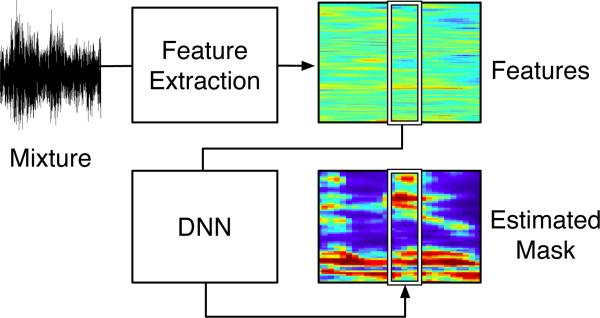
To evaluate the effects of noise perturbation, we use a fixed system for mask estimation and compare the quality of estimated masks as well as the resynthesized speech that are derived from the masked T-F representations of noisy speech. While comparison between an estimated mask and an ideal mask reveals the spectrotemporal distribution of estimation errors, resythesized speech can be directly compared to clean speech. As mentioned in Section 1, we use the IRM as the target of supervised learning. The IRM is computed from the 64-channel cochleagrams of premixed clean speech and noise. The cochleagram is a time-frequency representation of a signal (Wang and Brown, 2006). We use a 20 ms window and a 10 ms window shift to compute cochleagram in this study. We perform IRM estimation using a deep neural network (DNN) and a set of acoustic features. Recent studies have shown that DNN is a strong classifier for ASR (Mohamed et al., 2012) and speech separation (Wang and Wang, 2013; Xu et al., 2014). As shown in Fig. 1, acoustic features are extracted from a mixture sampled at 16 kHz, and then sent to a DNN for mask prediction.

Figure 1.

Diagram of the proposed system.

We use classification accuracy, hit minus false-alarm (HIT–FA) rate and short-time objective intelligibility (STOI) score (Taal et al., 2011) as three criteria for measuring the quality of the estimated IRM. Since the first two criteria are defined for binary masks, we calculate them by binarizing a ratio mask to a binary one. In this study, we follow Equation 3 and Equation 1.

$$\mathrm{SNR}(t,f)=10lo{g}_{10}\left(\frac{\mathrm{IRM}{(t,f)}^2}{1-\mathrm{IRM}{(t,f)}^2}\right)$$ (3)

During the mask conversion, the LC is set to be 5 dB lower than the SNR of a given mixture. The three criteria evaluate the estimated IRM from three different perspectives. Classification accuracy computes the percentage of correctly labeled T-F units in a binary mask. In HIT–FA, HIT refers to the percentage of correctly classified target-dominant T-F units and FA refers to the percentage of wrongly classified interference-dominant T-F units. HIT–FA rate is well correlated with human speech intelligibility (Kim et al., 2009). In addition, STOI is computed by comparing the the short-time envelopes of clean speech and resynthesized speech obtained from IRM masking, and it is a standard objective metric of speech intelligibility (Taal et al., 2011).

3. Noise perturbation

The goal of noise perturbation is to expand noise segments to cover unseen scenarios so that the overfitting problem is mitigated in supervised speech separation. A reasonable and straightforward idea for noise expansion is to reverse each noise signal in time. We have evaluated this idea and unfortunately adding reversed noises does not improve speech separation results. We conjecture that the spectrogram of a noise segment may be a better domain to apply perturbation. A recent study has found that three perturbations on speech samples in the spectrogram domain improve ASR performance (Kanda et al., 2013). These perturbations were used to expand the speech samples so that more speech patterns are observed by a classifier. The three perturbations are introduced below. Unlike this study, we perturb noise samples instead of perturbing speech samples, as we are dealing with highly nonstationary noises.

3.1. Noise Rate (NR) perturbation

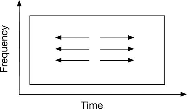
Speech rate perturbation, a way of speeding up or slow down speech, is used to expand training utterances during the training of an ASR system. In our study, we extend the method to vary the rate of nonstationary noises. We increase or decrease noise rate by factor γ. When a noise rate is being perturbed, the value of γ is randomly selected from an interval [γ_min, 2−γ_min]. The effect of NR perturbation on a spectrogram is shown in Fig. 2.

Figure 2.

Illustration of noise rate perturbation.

3.2. Vocal Tract Length (VTL) perturbation

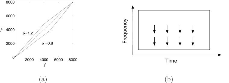
VTL perturbation has been used in ASR to cover the variation of vocal tract length among speakers. A recent study suggests that VTL perturbation improves ASR performance (Jaitly and Hinton, 2013). VTL perturbation essentially compresses or stretches the medium and low frequency components of an input signal. We use VTL perturbation as a method of perturbing a noise segment. Specifically, we follow the algorithm in (Jaitly and Hinton, 2013) to perturb noise signals:

$$f^{\prime }=\{\begin{array}{cc}f\alpha ,\hfill & \text{if}f\le F_{hi}\frac{min(\alpha ,1)}{\alpha }\hfill \\ \frac{S}{2}-\frac{\frac{S}{2}-F_{hi}min(\alpha ,1)}{\frac{S}{2}-F_{hi}\frac{min(\alpha ,1)}{\alpha }}(\frac{S}{2}-f),\hfill & \text{otherwise}\hfill \end{array}\phantom{\}}$$ (4)

where α is the wrapping factor, S is the sampling rate, and F_hi controls the cutoff frequency. Fig. 3(a) shows how VTL perturbation compresses or stretches a portion of a spectrogram. The effect of VTL perturbation is visualized in Fig. 3(b).

Figure 3.

(a) Mapping function for vocal tract length perturbation. The frequencies below a cutoff are stretched if α > 1, and compressed if α < 1. (b) Illustration of vocal tract length perturbation. The medium and low frequencies are compressed in this case.

3.3. Frequency perturbation

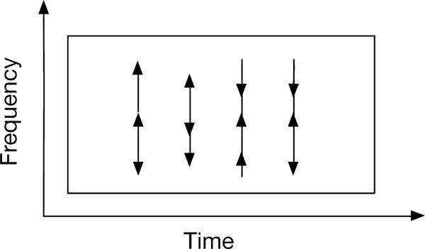
When frequency perturbation is applied, frequency bands of a spectrogram are randomly shifted upward or downward. We use the method described in (Kanda et al., 2013) to randomly perturb noise samples. Frequency perturbation takes three steps. First, we randomly assign a value to each T-F unit, which is drawn from a uniform distribution.

$$r(f,t)\sim U(-1,1)$$ (5)

Then we derive the perturbation factor δ(f, t) by averaging the assigned values of neighboring time-frequency units. This averaging step avoids large oscillations in spectrogram.

$$\delta (f,t)=\frac{\lambda }{(2p+1)(2q+1)}\sum _{f^{\prime }=f-p}^{f+p}\sum _{t^{\prime }=t-q}^{t+q}r(f^{\prime },t^{\prime })$$ (6)

where p and q control the smoothness of the perturbation, and λ controls the magnitude of the perturbation. These tunable parameters are decided experimentally. Finally the spectrogram is perturbed as follows.

$$\tilde{S}(f,t)=S(f+\delta (f,t),t)$$ (7)

where S(f, t) represents the original spectrogram and S̃(f, t) is the perturbed spectrogram. Interpolation between neighboring frequencies is used when δ(f, t) is not an integer. The effect of frequency perturbation is visualized in Fig. 4.

Figure 4.

Illustration of frequency perturbation.

4. Experimental results

4.1. Experimental setup

We use the IEEE corpus recorded by a male speaker (IEEE, 1969) and six nonstationary noises from the DEMAND corpus (Thiemann et al., 2013) to create mixtures. All signals are sampled at 16 KHz. Note that all recordings of the DEMAND corpus are made with a 16-channel microphone array, we use only one channel of the recordings since this study is on monaural speech separation.

The DEMAND corpus has six categories of noises. We choose one noise from each category to represent distinct environments. The six nonstationary noises, each is five-minute long, are described as follows.

1. The “Street” category:

   • The SCAFE noise, recorded in the terrace of a cafe at a public square.
2. The “Domestic” category:

   • The DLIVING noise, recorded inside a living room.
3. The “Office” category:

   • The OMEETING noise, recorded in a meeting room.
4. The “Public” category:

   • The PCAFETER noise, recorded in a busy office cafeteria.
5. The “Nature” category:

   • The NPARK noise, recorded in a well visited city park.
6. The “Transportation” category:

   • The TMETRO noise, recorded in a subway.

To create a mixture, we mix one IEEE sentence and one noise type at −5 dB SNR. This low SNR is selected with the goal of improving speech intelligibility in mind where there is not much to improve at higher SNRs (Healy et al., 2013). The training set uses 600 IEEE sentences and randomly selected segments from the first two minutes of a noise, while the test set uses another 120 IEEE sentences and randomly selected segments from the second two minutes of a noises. Therefore, the test set has different sentences and different noise segments from the training set. We create 50 mixtures for each training sentence by mixing it with 50 randomly selected segments from a given noise, which results in a training set containing 600×50 mixtures. The test set includes 120 mixtures. We train and test using the same noise type and SNR condition.

To perturb a noise segment, we first apply short-time Fourier transform (STFT) to derive noise spectrogram, where a frame length of 20 ms and a frame shift of 10 ms are used. Then we perturb the spectrogram and derive a new noise segment. To evaluate the three noise perturbations, we create five different training sets, each consists of 600×50 mixtures. We train a mask estimator for each training set and evaluate on a fixed test set (i.e. the 120 mixtures created from the original noises). The five training sets are described as follows.

1. Original Noise: All mixtures are created using original noises.

2. NR Perturbation: Half of the mixtures are created from NR perturbed noises, and the other half are from original noises.

3. VTL Perturbation: Half of the mixtures are created from VTL perturbed noises, and the other half are from original noises.

4. Frequency Perturbation: Half of the mixtures are created from frequency perturbed noises, and the other half are from original noises.

5. Combined: Half of the mixtures are created from applying three perturbations altogether, and the other half are from original noises.

The acoustic features we extract from mixtures are a complementary feature set (AMS + RASTAPLP + MFCC) (Wang et al., 2013) combined with gammatone filterbank (GFB) features. To compute 15-D AMS, we derive 15 modulation spectrum amplitudes from the decimated envelope of an input signal (Kim et al., 2009). 13-D RASTAPLP is derived by applying linear prediction analysis on the RASTA-filtered bark-scale power spectrum of an input signal (Hermansky and Morgan, 1994). We follow a standard procedure to compute 31-D MFCC. To derive GFB features, an input signal is passed to a 64-channel gammatone filterbank, the response signals are decimated to 100 Hz to form 64-D GFB features. After appending delta features, we end up with a feature set of 123×2 dimensions.

A four-hidden-layer DNN is employed to learn the mapping from acoustic features to the IRM. Each hidden layer of the DNN has 1024 rectified linear units (Nair and Hinton, 2010). To incorporate temporal context and obtain smooth mask estimation, we use 5 frames of features to estimate 5 frames of the IRM (Wang et al., 2014). As we use a 246-D feature set and the 64-channel IRM, the input layer of the DNN has 246×5 units and the output layer has 64×5 sigmoidal units. Since each frame of the mask is estimated 5 times, we take the average of the 5 estimates. We use mean squared error as the cost function. Hidden-layer dropout (Dahl et al., 2013) and adaptive stochastic gradient descent (AdaGrad) (Duchi et al., 2011) with a mini-batch size of 1024 are used to train the DNN. We set the dropout ratio to 0.2 and the initial learning rate of AdaGrad to 0.003. We train the DNN for 80 epochs and select the best epoch by cross validation.

4.2. Parameters of noise perturbation

In this section, three sets of experiments are carried out to explore the parameters used in the three perturbations to get the best performance. To facilitate parameter selection, we create five smaller training sets, following the same configuration in Section 4.1 except that we use 480 IEEE clean sentences to create 480×20 training mixtures. Another 120 IEEE sentences (different than the test ones in Section 4.1) are used to create 120 test mixtures only for the purpose of choosing parameter values (i.e. a development set). The speech separation performance is evaluated in term of STOI score.

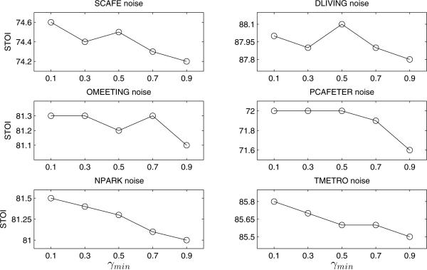
In NR perturbation, the only adjustable parameter is the rate γ. We can slow down a noise by setting γ < 1, or speed it up using γ > 1. To capture various noise rates, we randomly draw γ from an interval [γ_min, 2−γ_min]. We evaluate various intervals in term of speech separation performance. As shown in Fig. 5, the interval [0.1, 1.9] (i.e. γ_min = 0.1) gives the best performance for six noises.

Figure 5.

The effect of the minimum noise rate γ_min for NR perturbation.

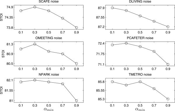
In VTL perturbation, there are two parameters: F_hi controls cutoff frequency and α the warping factor. F_hi is set to 4800 to roughly cover the frequency range of speech formants. We randomly draw α from an interval [α_min, 2−α_min] to systematically stretch or shrink the frequencies below the cutoff frequency. Fig. 6 shows the effects of different intervals on speech separation performance. The interval of [0.3, 1.7] (i.e. α_min = 0.3) leads to the best result for the majority of the noise types.

Figure 6.

The effect of the minimum wrapping factor α_min for VTL perturbation.

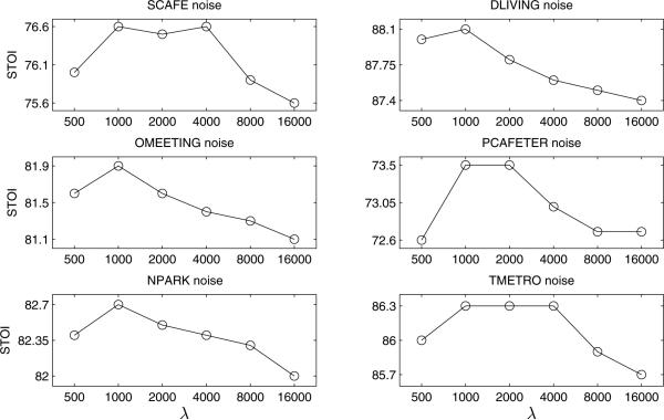
In frequency perturbation, a 161-band spectrogram derived from a noise segment is perturbed using the algorithm described in Section 3.3. We set p = 50 and q = 100 to avoid dramatic perturbation along time and frequency axes. We experiment with different perturbation intensity λ. As shown in Fig. 7, λ = 1000 achieves the best performance for the majority of the noise types.

Figure 7.

The effect of the perturbation intensity λ for frequency perturbation.

4.3. Evaluation results and comparisons

Before we evaluate the three perturbations, it is worth stressing that we are trying to apply noise perturbations to improve the performance of a strong baseline separation system, making further improvements harder. As described in Section 2, this baseline system trains a DNN to estimate the IRM. To demonstrate this, we compare our baseline system with a recently proposed supervised algorithm based on non-negative matrix factorization (NMF) (Ozerov et al., 2012; Mohammadiha et al., 2013). This algorithm is called active-set Newton algorithm (ASNA), which we denote as ASNA-NMF (Virtanen et al., 2013). We select ASNA-NMF as it outperforms many variants of supervised NMF algorithms (Virtanen et al., 2013). We set ASNA-NMF to use 1000 speech bases, 300 noise bases and 5 frames of magnitude spectra. For a fair comparison, we train ASNA-NMF on the first two minutes of a noise and 600 IEEE sentences, and test on the second two minutes of the noise and another 120 IEEE sentences. Table 1 shows the separation results of the baseline system and ASNA-NMF in terms of STOI. The DNN-based baseline produces significantly better results than ASNA-MNF for six noises at −5 dB SNR. On average, DNN-based ratio masking improves STOI by 10%, while ASNA-NMF improves STOI by 4%.

Table 1.

Comparison of DNN-based ratio masking (the baseline) with ASNA-NMF in terms of STOI (in %) for six noises at −5 dB.

Noise	SCAFE	DLIVING	OMEETING	PCAFETER	NPARK	TMETRO	Average
Method
Unprocessed	64.1	79.3	67.8	62.5	67.7	77.5	69.8
ASNA-NMF	67.5	82.4	73.4	66.0	72.5	81.2	73.8
DNN-IRM	73.7	87.5	80.0	71.4	80.2	85.9	79.8

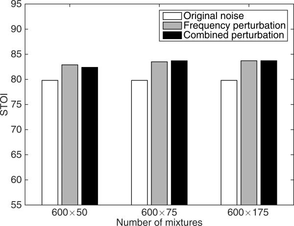
We evaluate the three perturbations with the parameter values selected in Section 4.2 and the five large training sets described in Section 4.1. The effects of noise perturbations on speech separation are shown in Table 2, Table 3 and Table 4, in terms of classification accuracy, HIT–FA rate and STOI score respectively. The results indicate that all three perturbations lead to better speech separation than the baseline where only the original noises are used. Frequency perturbation performs better than the other two perturbations. Compared to only using the original noises, the frequency perturbed training set on average increases classification accuracy, HIT–FA rate and STOI score by 8%, 11% and 3%, respectively. This indicates that noise perturbation is an effective technique for improving speech separation results. Combining three perturbations, however, does not lead to further improvement over frequency perturbation. We conjecture that frequency perturbation alone provides sufficient noise variations for generalization purposes. To verify this, we expand training by mixing each clean sentence with more noise segments. For the training sets using perturbed noises, we fix the number of mixtures created from original noises to 600×25, but vary the number of mixtures created from perturbed noises. Fig. 8 shows the average STOI results as the number is set to 600×25, 600×50, and 600×150. As the size of the training set increases, the combined method and frequency perturbation reach almost the same peak performance. We also observe that the speech separation performance does not benefit from a larger training set when no perturbation is used.

Table 2.

Classification accuracy (in %) for six noises at −5 dB

Noise	SCAFE	DLIVING	OMEETING	PCAFETER	NPARK	TMETRO	Average
Perturbation
Original Noise	73.0	84.0	80.0	70.3	82.7	80.3	78.4
NR Perturbation	80.2	88.5	85.3	77.9	88.5	85.1	84.2
VTL Perturbation	80.1	87.7	84.9	77.8	89.2	85.5	84.2
Frequency Perturbation	84.4	88.6	86.7	80.6	90.0	86.7	86.2
Combined	81.8	88.0	86.1	78.9	89.6	86.6	85.2

Table 3.

HIT–FA rate (in %) for six noises at −5 dB, where FA is shown in parentheses.

Noise	SCAFE	DLIVING	OMEETING	PCAFETER	NPARK	TMETRO	Average
Perturbation
Original Noise	55 (37)	70 (23)	65 (28)	50 (40)	69 (22)	63 (32)	62 (30)
NR Perturbation	64 (24)	77 (15)	72 (18)	60 (26)	77 (12)	72 (21)	70 (19)
VTL Perturbation	64 (24)	76 (16)	71 (19)	60 (27)	78 (10)	72 (21)	70 (20)
Frequency Perturbation	69 (17)	77 (14)	74 (15)	63 (21)	79 (9)	74 (18)	73 (16)
Combined	67 (21)	77 (15)	73 (16)	61 (25)	78 (10)	74 (18)	72 (18)

Table 4.

STOI (in %) of separated speech for six noises at −5 dB, where STOI of unprocessed mixtures is shown in parentheses.

Noise	SCAFE	DLIVING	OMEETING	PCAFETER	NPARK	TMETRO	Average
Perturbation
Original Noise	73.7 (64.1)	87.5 (79.3)	80.0 (67.8)	71.4 (62.5)	80.2 (67.7)	85.9 (77.5)	79.8 (69.8)
NR Perturbation	76.5 (64.1)	89.2 (79.3)	82.5 (67.8)	74.1 (62.5)	83.2 (67.7)	87.4 (77.5)	82.1 (69.8)
VTL Perturbation	76.1 (64.1)	88.7 (79.3)	82.2 (67.8)	74.0 (62.5)	83.6 (67.7)	87.2 (77.5)	82.0 (69.8)
Frequency Perturbation	78.2 (64.1)	89.1 (79.3)	83.3 (67.8)	75.1 (62.5)	84.1 (67.7)	87.8 (77.5)	82.9 (69.8)
Combined	77.0 (64.1)	88.6 (79.3)	82.7 (67.8)	74.7 (62.5)	83.8 (67.7)	87.6 (77.5)	82.4 (69.8)

Figure 8.

Average STOI (in %) of separated speech for six noises at −5 dB with respect to the number of training mixtures.

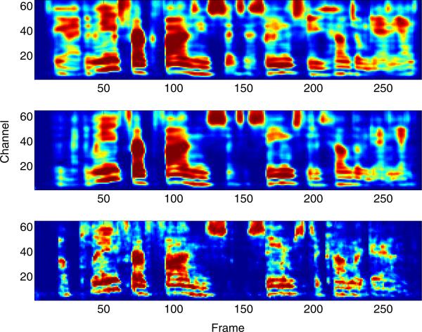
A closer look at Table 3 reveals that the contribution of frequency perturbation lies mainly in the large reduction in FA rate. This means that the problem of misclassifying noise-dominant T-F units as speech-dominant is mitigated. This effect can be illustrated by visualizing the masks estimated from the different training sets and the ground truth mask in Fig. 9 (e.g. around frame 150). When the mask estimator is trained with the original noises, it mistakenly retains the regions where target speech is not present, which can be seen by comparing the top and bottom plots of Fig. 9. Applying frequency perturbation to noises essentially exposes the mask estimator to more noise patterns and results in a more accurate mask estimator, which is shown in the middle plot of Fig. 9.

Figure 9.

Mask comparisons. The top shows a ratio mask obtained from training on original noises, the middle shows a mask obtained from training on frequency perturbed noise, and the bottom shows the IRM.

In addition, we show HIT–FA rate for voiced and unvoiced intervals in Table 5 and Table 6 respectively. We find that frequency perturbation is effective for both voiced and unvoiced intervals.

Table 5.

HIT–FA rate (in %) during voiced intervals, where FA is shown in parentheses.

Noise	SCAFE	DLIVING	OMEETING	PCAFETER	NPARK	TMETRO	Average
Perturbation
Original Noise	50 (44)	70 (26)	62 (33)	48 (45)	71 (24)	55 (42)	59 (36)
NR Perturbation	60 (32)	75 (21)	69 (24)	57 (33)	79 (15)	63 (33)	67 (26)
VTL Perturbation	62 (30)	75 (21)	70 (24)	60 (31)	80 (13)	65 (31)	69 (25)
Frequency Perturbation	66 (24)	76 (20)	72 (21)	62 (27)	80 (13)	67 (29)	70 (22)
Combined	65 (27)	76 (20)	72 (21)	61 (30)	80 (13)	68 (28)	70 (23)

Table 6.

HIT–FA rate (in %) during unvoiced intervals, where FA is shown in parentheses.

Noise	SCAFE	DLIVING	OMEETING	PCAFETER	NPARK	TMETRO	Average
Perturbation
Original Noise	48 (33)	61 (22)	59 (25)	41 (36)	57 (20)	61 (27)	54 (27)
NR Perturbation	54 (20)	70 (11)	64 (15)	48 (22)	62 (9)	68 (16)	61 (16)
VTL Perturbation	52 (21)	68 (13)	64 (15)	45 (24)	62 (8)	68 (16)	60 (16)
Frequency Perturbation	59 (12)	68 (11)	66 (11)	48 (18)	62 (6)	70 (13)	62 (12)
Combined	55 (18)	68 (12)	64 (13)	46 (22)	62 (8)	69 (14)	61 (14)

While classification accuracy and HIT–FA rate evaluate the estimated binary masks, STOI directly compares clean speech and the resynthesized speech. As shown in Table 4, frequency perturbation yields higher average STOI scores than using original noises with no perturbation and NR and VTL perturbations.

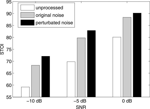
To evaluate the effectiveness of frequency perturbation at other SNRs, we carry out additional experiments at −10 dB and 0 dB input SNRs, where we use the same parameter values as for −5 dB SNR. Fig. 10 shows frequency perturbation improves speech separation in terms of STOI in each SNR condition. Also, we find that frequency perturbation remains the most effective among the three perturbations at −10 dB and 0 dB SNR.

Figure 10.

The effect of frequency perturbation in three SNR conditions. The average STOI scores (in %) across six noises are shown for unprocessed speech, separated speech by training on original noises, and separated speech by training on frequency perturbed noises.

All the above evaluations are conducted on unseen segments of the same nonstationary noises, corresponding to environment-specific speech separation (Hu and Loizou, 2010). Although not the focus of the present study, it is interesting to see how our mask estimator performs when evaluated on completely new noises. To get an idea, we evaluate two models trained with and without frequency perturbation. We use the same setting described in Section 4.1 except that we train on SCAFE noise and test on the other five noises. The results are shown in Table 7. As expected, the two models do not perform as well as in the matched noise case. But they still significantly improve STOI over unprocessed mixtures. Table 7 also shows that the model with frequency perturbation generalizes better to new noises than the model without perturbation.

Table 7.

STOI (in %) of separated speech for five unmatched noises at −5 dB, where STOI of unprocessed mixtures is shown in parentheses.

Test Noise	DLIVING	OMEETING	PCAFETER	NPARK	TMETRO
Training Noise
Matched noise (original noise)	87.5 (79.3)	80.0 (67.8)	71.4 (62.5)	80.2 (67.7)	85.9 (77.5)
Matched noise (perturbation)	89.1 (79.3)	83.3 (67.8)	75.1 (62.5)	84.1 (67.7)	87.8 (77.5)
SCAFE (original noise)	84.8 (79.3)	70.7 (67.8)	70.2 (62.5)	72.1 (67.7)	84.7 (77.5)
SCAFE (perturbation)	86.2 (79.3)	73.2 (67.8)	74.0 (62.5)	80.0 (67.7)	86.6 (77.5)

Finally, to evaluate the effect of frequency perturbation on multi-condition training, we test on SCAFE noise using another two models trained on the other five noises at −5 dB SNR. The first model is trained with 600 × 30 × 5 mixtures created using the five original noises, where each sentence is mixed with each noise type 30 times. The second model is trained with the same number of mixtures where one half are created using original noises and the other half are created using perturbed noises. The STOI of unprocessed mixtures, separated speech using the first model and separated speech using the second model are 64.1%, 75.5% and 78.4%, respectively. This indicates that frequency perturbation also improves generalization in multi-condition training.

5. Concluding remarks

In this study, we have explored the effects of noise perturbation on supervised monaural speech separation at low SNR levels. As a training set is usually created from limited speech and noise resources, a classifier likely overfits the training set and makes poor predictions on a test set, especially when background noise is highly nonstationary. We suggest to expand limited noise resources by noise perturbation.

We have evaluated three noise perturbations with six nonstationary noises recorded from daily life for speech separation. The three are noise rate, VTL, and frequency perturbations. When a DNN is trained on a data set which utilizes perturbed noises, the quality of the estimated ratio mask is improved as the classifier has been exposed to more scenarios of noise interference. In contrast, a mask estimator learned from a training set that only uses original noises tends to make more false alarm errors (i.e. higher FA rate), which is detrimental to speech intelligibility (Yu et al., 2014). The experimental results show that frequency perturbation, which randomly perturbs the noise spectrogram along frequency, almost uniformly gives the best speech separation results among the three perturbations examined in this study in terms of classification accuracy, HIT–FA rate and STOI score.

Finally, this study adds another technique to deal with the generalization problem in supervised speech separation. Previous studies use model adaptation (Han and Wang, 2013) and extensive training (Wang and Wang, 2013) to deal with the mismatch of SNR conditions, noises and speakers between training and testing. Our study aims at situations with limited training noises, and provides an effective data augmentation method that improves generalization in nonstationary environments. The idea of signal perturbation may also be applicable to augmenting speech signals for improved generalization to different kinds of speech data, such as different speaking rates and styles.

Highlights.

• We have explored noise perturbation methods for improving generalization of supervised speech separation.

• We have evaluated three noise perturbation methods and find that frequency perturbation is the most effective in terms of improved objective speech separation metrics.

• Frequency perturbation mitigates the problem of mistaking noise patterns for speech patterns.

References

- Ahmadi M, Gross VL, Sinex DG. Perceptual learning for speech in noise after application of binary time-frequency masks. J. Acoust. Soc. Am. 2013;133:1687–1692. doi: 10.1121/1.4789896. [DOI] [PMC free article] [PubMed] [Google Scholar]
- Bregman AS. Auditory scene analysis: The perceptual organization of sound. MIT Press; Cambridge MA: 1990. [Google Scholar]
- Brungart DS, Chang PS, Simpson BD, Wang DL. Isolating the energetic component of speech-on-speech masking with ideal time-frequency segregation. J. Acoust. Soc. Am. 2006;120:4007–4018. doi: 10.1121/1.2363929. [DOI] [PubMed] [Google Scholar]
- Chen J, Wang Y, Wang DL. Noise perturbation improves supervised speech separation. Proc. LVA/ICA. 2015:83–90. [Google Scholar]
- Ciresan D, Meier U, Schmidhuber J. Multi-column deep neural networks for image classification. Proc. CVPR. 2012:3642–3649. doi: 10.1016/j.neunet.2012.02.023. [DOI] [PubMed] [Google Scholar]
- Dahl GE, Sainath TN, Hinton GE. Improving deep neural networks for LVCSR using rectified linear units and dropout. Proc. ICASSP. 2013:8609–8613. [Google Scholar]
- Duchi J, Hazan E, Singer Y. Adaptive subgradient methods for online learning and stochastic optimization. The Journal of Machine Learning Research. 2011;12:2121–2159. [Google Scholar]
- Ephraim Y, Malah D. Speech enhancement using a minimum-mean square error short-time spectral amplitude estimator. IEEE Trans. Acoust., Speech, Sig. Process. 1984;32:1109–1121. [Google Scholar]
- Erkelens JS, Hendriks RC, Heusdens R, Jensen J. Minimum mean-square error estimation of discrete fourier coefficients with generalized gamma priors. IEEE Trans. Audio, Speech, Lang. Process. 2007;15:1741–1752. [Google Scholar]
- Han K, Wang D. Towards generalizing classification based speech separation. IEEE Trans. Audio, Speech, Lang. Process. 2013;21:168–177. [Google Scholar]
- Healy EW, Yoho SE, Wang Y, Wang DL. An algorithm to improve speech recognition in noise for hearing-impaired listeners. J. Acoust. Soc. Am. 2013;134:3029–3038. doi: 10.1121/1.4820893. [DOI] [PMC free article] [PubMed] [Google Scholar]
- Hermansky H, Morgan N. RASTA processing of speech. IEEE Trans. Speech, Audio Process. 1994;2:578–589. [Google Scholar]
- Hu Y, Loizou PC. Environment-specific noise suppression for improved speech intelligibility by cochlear implant users. J. Acoust. Soc. Am. 2010;127:3689–3695. doi: 10.1121/1.3365256. [DOI] [PMC free article] [PubMed] [Google Scholar]
- IEEE IEEE recommended practice for speech quality measurements. IEEE Trans. Audio Electroacoust. 1969;17:225–246. [Google Scholar]
- Jaitly N, Hinton GE. Vocal Tract Length Perturbation (VTLP) improves speech recognition. Proc. ICML Workshop on Deep Learning for Audio, Speech and Lang. Process. 2013 [Google Scholar]
- Jensen J, Hendriks RC. Spectral magnitude minimum mean-square error estimation using binary and continuous gain functions. IEEE Trans. Audio, Speech, Lang. Process. 2012;20:92–102. [Google Scholar]
- Kanda N, Takeda R, Obuchi Y. Elastic spectral distortion for low resource speech recognition with deep neural networks. Proc. ASRU. 2013:309–314. [Google Scholar]
- Kim G, Lu Y, Hu Y, Loizou PC. An algorithm that improves speech intelligibility in noise for normal-hearing listeners. J. Acoust. Soc. Am. 2009;126:1486–1494. doi: 10.1121/1.3184603. [DOI] [PMC free article] [PubMed] [Google Scholar]
- LeCun Y, Bottou L, Bengio Y, Haffner P. Gradient-based learning applied to document recognition. Proc. of the IEEE. 1998;86:2278–2324. [Google Scholar]
- Li N, Loizou PC. Factors influencing intelligibility of ideal binary-masked speech: Implications for noise reduction. J. Acoust. Soc. Am. 2008;123:1673–1682. doi: 10.1121/1.2832617. [DOI] [PMC free article] [PubMed] [Google Scholar]
- Mohamed A, Dahl GE, Hinton GE. Acoustic modeling using deep belief networks. IEEE Trans. Audio, Speech, Lang. Process. 2012;20:14–22. [Google Scholar]
- Mohammadiha N, Smaragdis P, Leijon A. Supervised and unsupervised speech enhancement using nonnegative matrix factorization. IEEE Trans. Audio, Speech, Lang. Process. 2013;21:2140–2151. [Google Scholar]
- Nair V, Hinton GE. Rectified linear units improve restricted boltzmann machines. Proc. ICML. 2010:807–814. [Google Scholar]
- Narayanan A, Wang D. Ideal ratio mask estimation using deep neural networks for robust speech recognition. Proc. ICASSP. 2013:7092–7096. [Google Scholar]
- Ozerov A, Vincent E, Bimbot F. A general flexible framework for the handling of prior information in audio source separation. IEEE Trans. Audio, Speech, Lang. Process. 2012;20:1118–1133. [Google Scholar]
- Taal CH, Hendriks RC, Heusdens R, Jensen J. An algorithm for intelligibility prediction of time-frequency weighted noisy speech. IEEE Trans. Audio, Speech, Lang. Process. 2011;19:2125–2136. [Google Scholar]
- Thiemann J, Ito N, Vincent E. The diverse environments multichannel acoustic noise database: A database of multichannel environmental noise recordings. J. Acoust. Soc. Am. 2013;133:3591. [Google Scholar]
- Virtanen T, Gemmeke JF, Raj B. Active-set newton algorithm for overcomplete non-negative representations of audio. IEEE Trans. Audio, Speech, Lang. Process. 2013;21:2277–2289. [Google Scholar]
- Wang DL, Brown GJ, editors. Computational auditory scene analysis: Principles, algorithms and applications. Wiley-IEEE Press; Hoboken NJ: 2006. [Google Scholar]
- Wang DL, Kjems U, Pedersen MS, Boldt JB, Lunner T. Speech intelligibility in background noise with ideal binary time-frequency masking. J. Acoust. Soc. Am. 2009;125:2336–2347. doi: 10.1121/1.3083233. [DOI] [PubMed] [Google Scholar]
- Wang Y, Han K, Wang DL. Exploring monaural features for classification-based speech segregation. IEEE Trans. Audio, Speech, Lang. Process. 2013;21:270–279. [Google Scholar]
- Wang Y, Narayanan A, Wang DL. On training targets for supervised speech separation. IEEE/ACM Trans. Audio, Speech, Lang. Process. 2014;22:1849–1858. doi: 10.1109/TASLP.2014.2352935. [DOI] [PMC free article] [PubMed] [Google Scholar]
- Wang Y, Wang DL. Towards scaling up classification-based speech separation. IEEE Trans. Audio, Speech, Lang. Process. 2013;21:1381–1390. [Google Scholar]
- Xu Y, Du J, Dai L-R, Lee C-H. An experimental study on speech enhancement based on deep neural networks. IEEE Signal Process. Lett. 2014;21:65–68. [Google Scholar]
- Yu C, Wójcicki KK, Loizou PC, Hansen JH, Johnson MT. Evaluation of the importance of time-frequency contributions to speech intelligibility in noise. J. Acoust. Soc. Am. 2014;135:3007–3016. doi: 10.1121/1.4869088. [DOI] [PMC free article] [PubMed] [Google Scholar]