

ABSTRACT
For next‐generation sequencing technologies, sufficient base‐pair coverage is the foremost requirement for the reliable detection of genomic variants. We investigated whether whole‐genome sequencing (WGS) platforms offer improved coverage of coding regions compared with whole‐exome sequencing (WES) platforms, and compared single‐base coverage for a large set of exome and genome samples. We find that WES platforms have improved considerably in the last years, but at comparable sequencing depth, WGS outperforms WES in terms of covered coding regions. At higher sequencing depth (95x–160x), WES successfully captures 95% of the coding regions with a minimal coverage of 20x, compared with 98% for WGS at 87‐fold coverage. Three different assessments of sequence coverage bias showed consistent biases for WES but not for WGS. We found no clear differences for the technologies concerning their ability to achieve complete coverage of 2,759 clinically relevant genes. We show that WES performs comparable to WGS in terms of covered bases if sequenced at two to three times higher coverage. This does, however, go at the cost of substantially more sequencing biases in WES approaches. Our findings will guide laboratories to make an informed decision on which sequencing platform and coverage to choose.
Keywords: exome sequencing, genome sequencing, coverage
Background
Whole‐exome sequencing (WES) has been adopted as a standard approach within genetic research; however, the implementation in clinical settings has been much slower. This is in part due to the fact that clinical applications are more demanding in terms of quality and robustness of the experiment than research applications. Novel clinical tests are typically required to perform as well or better than existing clinical tests on sensitivity and specificity. A major concern for the implementation of WES in the clinic is the reduced sensitivity as compared with gold‐standard Sanger sequencing at particular regions [Strom et al., 2014]. Although WES is much more sensitive on an exome‐wide scale, the sensitivity may be low at particular regions due to locus‐specific features or sequencing bias [Ross et al., 2013]. Fine‐tuning or improvements of mapping and variant calling software can resolve some of these false negatives [Liu et al., 2013; Park et al., 2014]. However, the most prominent reason for not calling variants is a lack of sufficient sequence coverage [Parla et al., 2011; Sulonen et al., 2011; Dewey et al., 2014], which cannot be resolved by improved algorithms.
Early comparisons of whole‐exome capture kits showed that all were able to capture around 80% of the human consensus‐coding sequence regions at a minimal coverage of 20x [Parla et al., 2011]. For the majority of low‐coverage regions, this could be attributed to an extreme GC content of the captured region as these regions are both difficult to capture as well as sequence [Hoischen et al., 2010; Benjamini and Speed, 2012]. This initial lack of sequence coverage for a significant proportion of the exome has spurred clinical laboratories to develop custom gene panels, or custom exome captures in order to achieve better capture performance, especially for known disease genes [Xue et al., 2014]. Current‐day exome enrichment designs try to circumvent the problem of capturing difficult regions by designing capture probes close to the region of interest. In combination with long paired‐end reads, this allows one to also sequence regions adjacent to the capture targets, that is, the actual region on interest. Comparisons performed for earlier capture kits are therefore not representative of current‐day standards in sequencing and capture technologies. Moreover, most of the published studies have compared coverage of capture targets rather than coding regions that is more relevant to clinical applications [Clark et al., 2011; Parla et al., 2011].
The cost of whole‐genome sequencing (WGS) is becoming less prohibitive for applying WGS as a clinical test [Hayden, 2014], and pilot studies have already been performed [Lupski et al., 2010; Jiang et al., 2013; Gilissen et al., 2014; Soden et al., 2014]. Although the major advantage of WGS over WES is its ability to also sequence noncoding DNA, WGS is also expected to outperform WES in the coding regions as WGS does not involve capture methods that can introduce bias. This improved coverage may make WGS a more suitable clinical test than WES. However, whether WGS indeed does perform better than WES, remains unclear. Jiang et al. (2013) performed one of the first direct comparisons of sequence coverage between WGS and WES. However, the study [Jiang et al., 2013] included only 10 WGS and 10 WES samples from a single platform and compared average exon coverage. A comparison of two WGS platforms for 56 genes concluded that current WGS platforms are unable to cover 10%–19% of genes to acceptable standards for SNV discovery [Dewey et al., 2014]. However, a direct comparison to current‐day exome sequencing was omitted. A comparison of WES and WGS for variant calling showed that both current WES experiments as well as WGS are unable to identify all variants [Clark et al., 2011]. It remained unclear however what proportion was due to intrinsic lack of sequence coverage, and which proportion may be amendable by improved variant detection.
Here, we focus on the coverage capability of the latest WES and WGS technologies in protein‐coding regions and investigate different technological biases. In particular, we look at the potential for clinical application by comparing the ability of WES and WGS to fully cover clinically relevant disease genes at a depth sufficient for reliable variant calling (≥20x). We provide a comprehensive comparison of base‐pair coverage and read distribution of the human exome of a wide array of high‐coverage samples generated by the most commonly used WES and WGS platforms.
Materials and Methods
Whole‐Exome Sequencing
Exome sequencing samples were collected for two current mainstream technologies. We selected 2 × 12 exome libraries captured with the Agilent SureSelect V4 kit (Agilent, Santa Clara, CA) sequenced by the Beijing Genomics Institute (BGI) in Copenhagen on an Illumina HiSeq system (Illumina, San Diego, CA) with 101 bp paired‐end reads. The first set contained samples sequenced to an average coverage of 78x and the second set were different samples sequenced at 160x. An additional 12 libraries were captured with the latest Agilent SureSelect V5 capture kit and sequenced by the Charité university clinic Berlin to an average coverage of 100x on an Illumina HiSeq system using 100 bp paired‐end reads. For NimbleGen, we selected 12 libraries captured by the latest NimbleGen SeqCap V3 and sequenced on an Illumina HiSeq using 101 bp paired‐end reads at 95x average coverage at the Duke Genome Centre (Table 1). DNA from all samples was derived from blood.
Table 1.
Overview of Tested Datasets, Average Coverage, Used Sequencing Systems, and Enrichment Kits
| Sequencing platform | Enrichment/library | Average exome coverage | Coverage range | # Samples |
| Illumina HiSeq | Agilent SureSelect V4 | 77.92 | 70–90 | 12 |
| Illumina HiSeq | Agilent SureSelect V4 | 159.92 | 151–170 | 12 |
| Illumina HiSeq | Agilent SureSelect V5 | 100.17 | 81–117 | 12 |
| Illumina HiSeq | NimbleGen SeqCap V3 | 94.50 | 92–97 | 12 |
| Complete Genomics | Whole genome | 44.17 | 41–48 | 12 |
| Complete Genomics | Whole genome | 87.42 | 83–95 | 12 |
| Illumina HiSeq | Whole genome | 28.09 | 26–30 | 11 |
| Illumina HiSeq | Whole genome | 56.20a | 56–57 | 5 |
| Illumina X Ten | Whole genome | 39.58 | 30–47 | 12 |
Columns depict (from left to right) the sequencing platform that was used; the exome enrichment kit or library preparation that were used; the average coverage across the RefSeq exome; the range of coverage; the number of samples used in the analysis.
aFor comparison, the 28.09x genomes sequenced on the Illumina HiSeq system are merged to resemble five samples sequenced to 56.20x coverage.
Whole‐Genome Sequencing
Samples for WGS were likewise collected for three mainstream sequencing platforms. We selected 12 whole genomes of four parent–child trios that were sequenced by Complete Genomics to an average coverage of 87x using 35 bp paired‐end reads [Drmanac et al., 2010] and were additionally downsampled to 44x. We obtained 11 additional WGS samples sequenced on an Illumina HiSeq at Duke genomics core at 28x using 101 bp paired‐end reads. For coverage comparisons, the single base pair coverage counts of these samples were merged into five samples to resemble an average of 56x coverage. Additionally, we gathered 12 WGS samples from the Charité university clinic Berlin sequenced on an Illumina X Ten system at Macrogen Inc. with the TruSeq Nano DNA (350) to an average coverage of 40x using 150 bp paired‐end reads (Table 1).
Mapping of the Reads
All exome samples were aligned to the hg19/GRCh37 assembly of the human reference genome by the Burrows Wheeler Aligner (BWA) [Li and Durbin, 2009] by the respective sequencing center. Illumina HiSeq samples were aligned by BWA version 0.5.9; Illumina x Ten samples were aligned with ISAAC version 1.0 and Complete Genomics samples were aligned using Complete Genomics assembly software version 2.4.0.43. We did not take into account whether duplicate reads were excluded during the mapping process.
Definition of the Exome and Gene Sets
In order to compute coverage of human protein‐coding regions, we defined a consensus exome by merging locations of protein‐coding regions using the hg19 assembly transcripts of the NCBI RefSeq database (Release 60) [Pruitt et al., 2014]. As an alternative to the more conservative RefSeq regions, we used the EMBL‐EBI Ensembl (Release 77) [Flicek et al., 2014] regions, which contains more gene models from multiple sources. The RefSeq and Ensembl transcripts were downloaded from the UCSC table browser (http://genome.ucsc.edu/) [Karolchik et al., 2004] and converted by a custom Java program to bed format. The merging of overlapping regions was done by the merge function from the BEDTools software package v.2.19.1 [Quinlan and Hall, 2010]. Only protein‐coding regions annotated to chromosomes 1–22 and X were used in the coverage comparison. This resulted in a 33.3‐Mb RefSeq and a 35.1‐Mb Ensembl‐based consensus exome (Supp. Table S1).
The computation of transcript coverage was based on two sets of disease genes. The first set consisted of 56 genes recommended by the American College of Medical Genetics (ACMG) for pathogenic variant discovery [Green et al., 2013]. The second set, named hereafter OMIM+, consisted of 2,759 genes derived from the Online Mendelian Inheritance in Man (OMIM) Morbid Map (Online Mendelian Inheritance in Man) and the Clinical Genome Database (CGD) [Solomon et al., 2013]. The OMIM Morbid Map and CGD are manually curated databases and catalogue disease genes published in literature. Only genes with the highest OMIM level of evidence were included (entries with a known molecular basis of the disorder). For both gene sets, rather than calculating consensus‐coding regions, we selected the longest transcript of each gene. This provides a biologically more meaningful and practically more relevant comparison. The regions of the transcripts were extracted from the RefGene transcript list (downloaded from the UCSC table browser, http://genome.ucsc.edu/) [Karolchik et al., 2004]. The base‐pair coverage for each transcript at different coverage intervals was calculated using custom java programs.
Coverage Calculation of the Exome
Single base‐pair coverage was calculated, based on the BAM‐files, with the use of the coverage function of the BEDTools package v.2.19.1 [Quinlan and Hall, 2010]. For Complete Genomics, the reference coverage files were converted to tabix format and the coverage of the regions was extracted via the tabix tool from the SAMtools package v0.1.19 [Li et al., 2009].
Coverage Calculation of Human Gene Mutation Database Mutations
To analyze coverage of known pathogenic mutations, 96,377 single‐nucleotide mutations from the Human Gene Mutation Database (HGMD; professional version) were downloaded on 09‐2014 [Stenson et al., 2014]. Mutations were then intersected with RefSeq (82076 SNVs) and Ensembl (82353) coding regions covered at ≥20x using the BEDTools software package v.2.19.1 [Quinlan and Hall, 2010].
Assessment of Systematic Biases
First, we calculated three different metrics in order to assess potential technological biases. The evenness score describes the uniformity of the base coverage over target regions and was calculated according to the method by Mokry et al. (2010). The score is normalized to the average coverage and therefore depicts the quality of a targeted genome section. The evenness score is 100% for completely uniform coverage where an extreme nonuniform distribution approaches a score of 0%. The average coverage for the exome was computed using a custom Java program.
Second, we also evaluated coverage bias for genes located on the positive and negative strand. We extracted the orientation for all genes from the NCBI RefSeq database (Release 60) [Pruitt et al., 2014]. Consistent with the transcript analysis, we selected the longest transcript of each gene. For each transcript, we computed the percentage of base pairs not covered at a coverage level ranging from 20‐ to 40‐fold and tested for coverage bias based on DNA strand (Mann–Whitney nonparametric U‐test).
Finally, we evaluated bias in the allele distributions of common heterozygous single‐nucleotide polymorphisms (SNPs). The list of protein‐coding single SNPs, based on the dbSNP database (build 138) [Sherry et al., 2001], was downloaded from the UCSC table browser (http://genome.ucsc.edu/) [Karolchik et al., 2004]. SNPs annotated with a population frequency above 10% were considered as common. In total, our set contained 15,153 common SNPs in protein‐coding regions. With the mpileup function from SAMtools v0.1.19 [Li et al., 2009], the nucleotide counts for each SNP location were extracted from the BAM files. SNPs with less than 16 reads were discarded to rule out distribution bias caused by low coverage. SNPs were considered heterozygous when the allele ration was between 10% and 90% based on the raw‐nucleotide counts. Difference in coverage was determined by the Mann–Whitney nonparametric U‐test and P values were corrected for multiple testing by the Benjamini–Hochberg procedure. On average, 4,307 (range [2,690–5,096]) heterozygous SNPs of our set were found per sample. For this analysis, we excluded the five Illumina genomes that were merged together to resemble 56.2x coverage. For the Complete Genomics data, the nucleotide counts for the common protein‐coding SNPs were extracted from the masterVarBeta files.
GC Content of Low‐Covered Regions
Based on the single base‐pair coverage, the RefSeq regions covered with less than 5x, between 5× and 10x and between 10× and 20x were selected. With the use of the nuc function from the BEDTools software package v.2.19.1 [Quinlan and Hall, 2010], the percentage G and C nucleotides of these regions could be extracted based on hg19 assembly of the human genome. The exome kit regions were corrected for targeted regions based on the capture probes locations as provided by the manufacturers.
Results
For our comparison, we evaluated three widely used exome capturing kits: Agilent SureSelect version 4 (Agilent V4), Agilent SureSelect version 5 (Agilent V5), and NimbleGen SeqCap version 3 (NimbleGen V3). Libraries for all aforementioned enrichment kits were sequenced on the commonly used Illumina HiSeq sequencer. Additionally, three WGS platforms were examined: Complete Genomics, Illumina HiSeq, and Illumina x Ten (Table 1). For all platforms, we evaluated the percentage of sufficiently (≥20x) covered protein‐coding regions based on RefSeq [Pruitt et al., 2014] and Ensembl [Flicek et al., 2014] annotated exons. Furthermore, the coverage in two clinically relevant transcript sets was assessed to study the potential for clinical application. Next to coverage, systematic biases such as nonuniform mapping of reads, unequal strand coverage, and deviations in allele distributions of common heterozygous SNPs were assessed.
Newer Exome Capture Kits Show a Clear Improvement in Exome Coverage
First, we compared the coverage of sequence libraries constructed by the exome kits (Table 1). We observed that libraries of the most recent Agilent V5 kit are able to capture on average 94.57% of RefSeq and 93.58% of Ensembl defined exome at ≥20x coverage, whereas the Agilent V4 libraries achieved 88.75% and 87.41% (Fig. 1; and Supp. Table S2). The difference between Agilent V4 and V5 is in part due to missing coding regions in the V4 capture design (Supp. Table S3). Deeper sequencing, on an Illumina HiSeq system, of the Agilent V4 libraries to 160x average depth increased the ≥20x‐covered exome to 94.10% for the refSeq exome and 92.79% for the Ensembl exome. However, by deeper sequencing, the average coverage did not surpass that of the Agilent V5. The NimbleGen V3 capture kit performed similar to the Agilent V5 with 95.83% and 94.49% covered at ≥20x. These results represent a marked improvement compared with previous generations of sequencing platforms that were able to capture at most 80.50% of the human consensus‐coding sequence regions [Parla et al., 2011].
Figure 1.
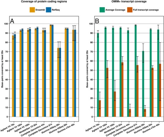
Coverage of the Ensembl and RefSeq annotated protein‐coding regions and (full) coverage of 2,759 clinically relevant OMIM+ genes. A: The percentage of base pairs of Ensembl (in yellow) and RefSeq (in blue) annotated protein‐coding regions covered by at least 20 reads for the tested platforms. B: Percentage of base pairs covered by at least 20 reads for the longest OMIM+ transcripts (in green). The red bars depict the percentage of the (longest) OMIM+ transcript base pairs that are fully covered by at least 20 reads.
WGS Provides a Better Exome Coverage than WES
Next, we assessed whether WGS indeed provides a better coverage of the RefSeq and Ensembl defined exomes. Both the 44x Complete Genomics and 56x Illumina HiSeq genomes achieved a much higher fraction of the exome covered at ≥20x than the 70x Agilent V4 (Fig. 1; Supp. Table S2). Only at a deeper average coverage of 160x, the results from the Agilent V4 libraries were comparable to much lower sequenced WGS (44–56x). Both Agilent V5 and NimbleGen V3 libraries achieved similar performance compared with the WGS, although be it at the cost of about two times more average coverage. Complete Genomics sequencing at high coverage (87x) outperformed all exome libraries with 98.40% and 98.58% coverage (Fig. 1; Supp. Table S2). Similar results were obtained when we compared only the coverage of 96377 HGMD mutations between the different platforms (Supp. Table S4) [Stenson et al., 2014].
Complete Coverage of Clinically Relevant Genes
From a clinical point of view, it is important to cover the sequence of disease genes as complete as possible. We analyzed the coverage for a set of 56 genes, recommended by the American College of Medical Genetics and Genomics (ACMG) for pathogenic variant discovery [Green et al., 2013]. This transcript set covers 198,482 nucleotides divided over 1,169 exons. We assessed the percentage of transcripts that are completely sequenced to a depth of ≥20x (Fig. 2; Supp. Table S5). With an average of 50.15%, the NimbleGen V3 libraries, achieved the highest average of fully covered transcripts captured for the enrichment kits. Genome performance was not obviously better than the exomes with on average 54% and 43% of fully covered transcripts for Complete Genomics 87x genomes and Illumina 56x genomes, respectively. The difference between the Complete Genomics 44x and 87x genomes was striking, with an average percentage of fully covered transcripts of 6.70% and 54.32%, respectively. Interestingly, for these genes, the difference in percentage of exome fraction covered at ≥20x was only 4.44%.
Figure 2.

Overview of 56 genes and the percentage of coding bases not covered at 20x. The boxplots depicting the percentage of bases not covered by at least 20x reads. For each of the 56 ACMG‐recommended genes, the coverage of the longest RefSeq transcript was analyzed. A: Shows the performance of all tested exome capture libraries. B: Shows the performance of the tested WGS platforms.
We extended our analysis to the coverage of 2,759 transcripts from the OMIM+ set (Fig. 1; Supp. Table S5). This set is much larger than the ACMG set and includes overall 6,374,161 nucleotides distributed across 38,498 exons. Due to the higher number of transcripts, a lower average number of nucleotides was covered at ≥20x compared with the ACMG set. However, for all platforms, the percentage of transcripts fully covered at ≥20x increased compared with the ACMG set. This may indicate that some of the ACMG genes are particularly difficult to sequence compared with other disease genes.
In addition, we explored GC ratios of insufficiently covered regions. The GC ratio of these regions was computed for regions with minimal (<5x), poor coverage (between 5× and 10x) and intermediate (between 10× and 20x) coverage (Supp. Table S6). Based on the genomic sequence of the RefSeq protein‐coding region, the average GC content is 51%. The mean GC content for annotated regions with minimal coverage, poor, and intermediate coverage was however 73.13%, 70.48%, and 64.43%, respectively, on average for exomes, and 72.78%, 70.40%, and 65.20% on average for Complete Genomics and Illumina HiSeq genomes.
Systematic Biases in Sequence Coverage
To investigate systematic biases in coverage, we compared the evenness of mapped reads across targets. As noted by Lam et al. (2012), less uniform coverage requires more overall sequencing to achieve a certain level of coverage for most of the genome. Moreover, uniform coverage is not only important in economic terms, but also for applications such as the detection of copy‐number variation and somatic variation. The evenness score of exome capture technologies was on average 74.6% (range [67.67%–78.32%]). Scores for Illumina HiSeq, x Ten, and Complete Genomics were very similar around 85% (range [78.39%–90.31%]) (Fig. 3A; Supp. Table S7).
Figure 3.

Assessments of three different sequence coverage biases. A: Evenness scores (a measure for uniform read mapping) for the different platforms based on the RefSeq annotated protein‐coding regions. B: The difference in average coverage at 20x of WGS libraries for RefSeq transcripts grouped by strand. The symbols + and – indicate average coverage level at the plus and minus strand. C: Idem for WES libraries. D: Density plot of allele ratio distribution for heterozygous SNPs. The green line depicts the ideal heterozygous allele ratio of 0.5.
To assess the observed reduction in evenness further, we evaluated whether transcripts on either the plus or minus strand were covered at equal proportions. The exome capture libraries provided significantly less coverage for genes on the minus strand compared with those on the plus strand (Fig. 3B). This effect becomes more apparent at higher exome coverage and was not present in the WGS data (Fig. 3C; Supp. Table S8). To further assess this, we studied the distribution of reads for heterozygous SNPs (minimal coverage of ≥20 reads) to see whether there was a systematic deviation from the ideal 50%–50% allele distribution. Exomes showed on average a deviation of 2.3% to the optimal 50%, whereas the whole‐genome datasets distribution deviated only 1.43% (P = 0.04; two‐sided Student's t‐test) (Fig. 3D; Supp. Table S9).
Discussion
High‐throughput sequencing techniques have shown a rapid development and made a significant impact on how genetic research is conducted. Scanning all genes simultaneously has led to the identification of a vast number of disease‐causing genes. Various studies have tried to determine what amount of sequence coverage is sufficient to reliable identify single‐nucleotide variants [Ajay et al., 2011; Clark et al., 2011; Sulonen et al., 2011; Meynert et al., 2014]. A challenge for this is that a comprehensive golden standard for variant calling is still under development [Strom et al., 2014; Zook et al., 2014], and that results may depend on the choice of variant caller and settings thereof. However, a prerequisite for reliable variant calling is sufficient sequence coverage.
In this study, we examined the latest WES and WGS platforms in terms of coverage of RefSeq [Pruitt et al., 2014] and Ensembl [Flicek et al., 2014] annotated regions (Table 1; Supp. Table S1). To increase robustness of our results, we used multiple replicates per approach. Although all of the samples were sequenced using standard sequencing protocols, site‐specific implementations may have an influence on the actual results. We conducted our comparison at a single base‐pair resolution and assessed biases in coverage for all technologies. We find that exome capture technology has significantly improved and that, at high‐average coverage (≥95x), the latest exome libraries are able to reliably cover close to 95% of the protein‐coding regions to a sequencing depth of at least 20x (Fig. 1; Supp. Table S2). Our choice of 20x coverage for reliable coverage stems from various published studies as well as our own experience. However, although results change for different thresholds, the overall differences between the platforms remain the same (Supp. Table S2).
We note that the definition of the exome naturally affects the outcome of this comparison [Bainbridge et al., 2011]. The absence of probes in enrichment kits restricts sequencing yield of regions when a more comprehensive exome definition is used. However, we find that in all but few exome libraries, a region will be sufficiently covered if a capture probe is in the vicinity. Exceptions to this occur in extreme GC regions, where genome sequencing may also suffer from loss of sequence coverage (Supp. Table S6). The differences in GC bias that we observed may be directly correlated to the number of PCR steps of the sequencing protocols that were used.
Full transcript coverage for clinically relevant disease genes was quite variable between replicate samples. Some platforms performed poor due to lower average coverage, but performed better with a lower coverage threshold for fully covered transcripts (Figs. 1 and 2; Supp. Table S5). Unexpectedly, the high‐coverage Agilent V5 samples also performed poor in this analysis. We suspect this may be due to performance differences between individual sequencing runs, rather than being intrinsic to the platform itself. Dewey et al. (2014) previously reported that 10% and 19% of 56 disease genes were not fully covered at an acceptable coverage of ≥10x by Illumina and Complete Genomics, respectively. In this study, a comparable 21% of the genes were not completely covered by at least 10 reads by Complete Genomics at 87.42x average coverage. However, this representation of the results does not do credit to the actual performance of these technologies as Illumina and Complete Genomics genomes achieve ≥10x coverage for 98.71% and 99.8% of the coding bases of this gene set (Supp. Table S10).
Next to sequence coverage, we also investigated several other important features to identify systematic biases. We found that genome sequencing performed better than exome sequencing in all of these comparisons, providing a more even coverage, no strand bias, and a higher proportion of transcripts covered completely (Fig. 3). Although these features may seem secondary to sequence coverage, they may have implications in a clinical setting where reliability and reproducibility of results is crucial. Also, for applications other than the identification of normal SNVs, these features are of importance. A more even coverage increases the sensitivity for detecting copy‐number variants [Medvedev et al., 2010; Szatkiewicz et al., 2013], and allele biases may hamper the detection of somatic variation.
The imperfect performance of previous generations of exome captures has spurred clinical laboratories to develop custom gene panels, or custom exome captures, to boost coverage of relevant disease genes. Recently published studies of gene panels show that these libraries are generally sequenced much deeper than WES and WGS libraries and cover in the range of 92.0%–98.7% of the regions by 10 or more reads (Supp. Table S11) [Glöckle et al., 2014; Qu et al., 2014; Vona et al., 2014; Wei et al., 2014; Zhao et al., 2015]. In comparison, the ACMG (56 genes) and OMIM+ (2759 genes) disease gene sets tested in this study shows comparable or better performance coverage for WES (ACMG range [95.95%–99.01%]; OMIM+ range [95.60%–98.02%]) and WGS (ACMG range [95.24%–99.80%]; OMIM+ range [93.00%–99.51%]) platforms at ≥10x (Supp. Table S10). This illustrates the potential of WES or WGS approaches for more generic clinical testing [Soden et al., 2014].
Conclusion
Both high‐coverage WES and WGS are able to generate sufficient coverage for reliable variant calling of 95% of the coding regions. Sequencing biases are however more prominent in WES data, and may hamper more advanced applications. WGS however offers the additional advantages that it allows more reliable detection of structural variants [Gilissen et al., 2014] and the identification of noncoding variation [Spielmann and Klopocki, 2013]. Although currently the costs of WES and WGS only differ by a factor 2–4 (depending on coverage), the additional data storage and computational burden may still make WES a convenient prescreening technology. Our findings will help laboratories to make an informed decision on which sequencing platform and what sequencing coverage to choose for their experiments.
Supporting information
Table S1. Overview of the RefSeq and Ensembl datasets used to define the human exome
Table S2. Overview of base‐pair coverage for different platforms and coverage thresholds
Table S3. Difference in Agilent SureSelect version 4 and 5 target regions
Table S4. Coverage summary of HGMD single nucleotide variants
Table S5. Coverage summary of ACMG and OMIM+ transcripts
Table S6. GC‐content of refSeq annotated regions per sequencing system
Table S7. Average evenness scores of coverage for the RefSeq annotated protein‐coding regions for the different exome and genome datasets
Table S8. Comparison of the average coverage of genes located on the plus and minus strand
Table S9. Allele ratio's for heterozygous SNPs
Table S10. Coverage summary of ACMG and OMIM+ transcripts
Table S11. Overview of coverage achieved by published gene‐panel sequencing studies
Acknowledgments
The authors would like to thank Maartje van de Vorst and Complete Genomics for assistance in the data analysis. We are very grateful to David Goldstein for sharing exome and genome datasets.
Author's contributions: Data analysis: S.H.L., C.G.; study design: C.G. and J.A.V.; data generation: M.S., S.M., and J.A.V; manuscript writing: S.H.L., C.G., and J.A.V.
Disclosure statement: The authors declare no competing interests.
Contract grant sponsors: The Netherlands Organization for Scientific Research (916‐14‐043 and SH‐271‐13); European Research Council (ERC Starting Grant DENOVO 281964).
Communicated by Mats Nilsson
References
- Ajay SS, Parker SCJ, Abaan HO, Fajardo KVF, Margulies EH. 2011. Accurate and comprehensive sequencing of personal genomes. Genome Res 21:1498–1505. [DOI] [PMC free article] [PubMed] [Google Scholar]
- Bainbridge MN, Wang M, Wu Y, Newsham I, Muzny DM, Jefferies JL, Albert TJ, Burgess DL, Gibbs RA. 2011. Targeted enrichment beyond the consensus coding DNA sequence exome reveals exons with higher variant densities. Genome Biol 12:R68. [DOI] [PMC free article] [PubMed] [Google Scholar]
- Benjamini Y, Speed TP. 2012. Summarizing and correcting the GC content bias in high‐throughput sequencing. Nucleic Acids Res 40:e72. [DOI] [PMC free article] [PubMed] [Google Scholar]
- Clark MJ, Chen R, Lam HYK, Karczewski KJ, Chen R, Euskirchen G, Butte AJ, Snyder M. 2011. Performance comparison of exome DNA sequencing technologies. Nat Biotechnol 29:908–914. [DOI] [PMC free article] [PubMed] [Google Scholar]
- Dewey FE, Grove ME, Pan C, Goldstein BA, Bernstein JA, Chaib H, Merker JD, Goldfeder RL, Enns GM, David SP, Pakdaman N, Ormond KE, et al. 2014. Clinical interpretation and implications of whole‐genome sequencing. JAMA 311:1035–1045. [DOI] [PMC free article] [PubMed] [Google Scholar]
- Drmanac R, Sparks AB, Callow MJ, Halpern AL, Burns NL, Kermani BG, Carnevali P, Nazarenko I, Nilsen GB, Yeung G, Dahl F, Fernandez A, et al. 2010. Human genome sequencing using unchained base reads on self‐assembling DNA nanoarrays. Science 327:78–81. [DOI] [PubMed] [Google Scholar]
- Flicek P, Amode MR, Barrell D, Beal K, Billis K, Brent S, Carvalho‐Silva D, Clapham P, Coates G, Fitzgerald S, Gil L, Girón CG, et al. 2014. Ensembl 2014. Nucleic Acids Res 42:D749–D755. [DOI] [PMC free article] [PubMed] [Google Scholar]
- Gilissen C, Hehir‐Kwa JY, Thung DT, van de Vorst M, van Bon BWM, Willemsen MH, Kwint M, Janssen IM, Hoischen A, Schenck A, Leach R, Klein R, et al. 2014. Genome sequencing identifies major causes of severe intellectual disability. Nature 511:344–347. [DOI] [PubMed] [Google Scholar]
- Glöckle N, Kohl S, Mohr J, Scheurenbrand T, Sprecher A, Weisschuh N, Bernd A, Rudolph G, Schubach M, Poloschek C, Zrenner E, Biskup S, et al. 2014. Panel‐based next generation sequencing as a reliable and efficient technique to detect mutations in unselected patients with retinal dystrophies. Eur J Hum Genet 22:99–104. [DOI] [PMC free article] [PubMed] [Google Scholar]
- Green RC, Berg JS, Grody WW, Kalia SS, Korf BR, Martin CL, McGuire AL, Nussbaum RL, O'Daniel JM, Ormond KE, Rehm HL, Watson MS, et al. 2013. ACMG recommendations for reporting of incidental findings in clinical exome and genome sequencing. Genet Med 15:565–574. [DOI] [PMC free article] [PubMed] [Google Scholar]
- Hayden EC. 2014. Is the $1000 genome for real? Nature 507(7492):294–295. [DOI] [PubMed] [Google Scholar]
- Hoischen A, Gilissen C, Arts P, Wieskamp N, van der Vliet W, Vermeer S, Steehouwer M, de Vries P, Meijer R, Seiqueros J, Knoers NVAM, Buckley MF, et al. 2010. Massively parallel sequencing of ataxia genes after array‐based enrichment. Hum Mutat 31:494–499. [DOI] [PubMed] [Google Scholar]
- Jiang YH, Yuen RK, Jin X, Wang M, Chen N, Wu X, Ju J, Mei J, Shi Y, He M, Wang G, Liang J, et al. 2013. Detection of clinically relevant genetic variants in autism spectrum disorder by whole‐genome sequencing. Am J Hum Genet 93:249–263. [DOI] [PMC free article] [PubMed] [Google Scholar]
- Karolchik D, Hinrichs AS, Furey TS, Roskin KM, Sugnet CW, Haussler D, Kent WJ. 2004. The UCSC Table Browser data retrieval tool. Nucleic Acids Res 2004:D493–D496. [DOI] [PMC free article] [PubMed] [Google Scholar]
- Lam HYK, Clark MJ, Chen R, Chen R, Natsoulis G, O'Huallachain M, Dewey FE, Habegger L, Ashley EA, Gerstein MB, Butte AJ, Ji HP, et al. 2012. Performance comparison of whole‐genome sequencing platforms. Nat Biotechnol 30:78–82. [DOI] [PMC free article] [PubMed] [Google Scholar]
- Li H, Durbin R. 2009. Fast and accurate short read alignment with Burrows–Wheeler transform. Bioinformatics 25:1754–1760. [DOI] [PMC free article] [PubMed] [Google Scholar]
- Li H, Handsaker B, Wysoker A, Fennell T, Ruan J, Homer N, Marth G, Abecasis G, Durbin R. 2009. The sequence alignment/Map format and SAMtools. Bioinformatics 25:2078–2079. [DOI] [PMC free article] [PubMed] [Google Scholar]
- Liu X, Han S, Wang Z, Gelernter J, Yang B‐Z. 2013. Variant callers for next‐generation sequencing data: a comparison study. PloS One 8:e75619. [DOI] [PMC free article] [PubMed] [Google Scholar]
- Lupski JR, Reid JG, Gonzaga‐Jauregui C, Deiros DR, Chen DCY, Nazareth L, Bainbridge M, Dinh H, Jing C, Wheeler DA, McGuire AL, Zhang F, et al. 2010. Whole‐genome sequencing in a patient with Charcot–Marie–Tooth neuropathy. N Engl J Med 362:1181–1191. [DOI] [PMC free article] [PubMed] [Google Scholar]
- Medvedev P, Fiume M, Dzamba M, Smith T, Brudno M. 2010. Detecting copy number variation with mated short reads. Genome Res 20:1613–1622. [DOI] [PMC free article] [PubMed] [Google Scholar]
- Meynert AM, Ansari M, FitzPatrick DR, Taylor MS. 2014. Variant detection sensitivity and biases in whole genome and exome sequencing. BMC Bioinformatics 15:247–258. [DOI] [PMC free article] [PubMed] [Google Scholar]
- Mokry M, Feitsma H, Nijman IJ, de Bruijn E, van der Zaag PJ, Guryev V, Cuppen E. 2010. Accurate SNP and mutation detection by targeted custom microarray‐based genomic enrichment of short‐fragment sequencing libraries. Nucleic Acids Res 38:e116. [DOI] [PMC free article] [PubMed] [Google Scholar]
- Online Mendelian Inheritance in Man OM‐NIoGM, Johns Hopkins University . Baltimore, MD.
- Park MH, Rhee H, Park JH, Woo HM, Choi BO, Kim BY, Chung KW, Cho YB, Kim HJ, Jung JW, Koo SK. 2014. Comprehensive analysis to improve the validation rate for single nucleotide variants detected by next‐generation sequencing. PLoS One 9:e86664. [DOI] [PMC free article] [PubMed] [Google Scholar]
- Parla JS, Iossifov I, Grabill I, Spector MS, Kramer M, McCombie WR. 2011. A comparative analysis of exome capture. Genome Biol 12:R97. [DOI] [PMC free article] [PubMed] [Google Scholar]
- Pruitt KD, Brown GR, Hiatt SM, Thibaud‐Nissen F, Astashyn A, Ermolaeva O, Farrell CM, Hart J, Landrum MJ, McGarvey KM, Murphy MR, O'Leary NA, et al. 2014. RefSeq: an update on mammalian reference sequences. Nucleic Acids Res 42:D756–D763. [DOI] [PMC free article] [PubMed] [Google Scholar]
- Qu LH, Jin X, Xu HW, Li SY, Yin ZQ. 2014. Detecting novel genetic mutations in Chinese Usher syndrome families using next‐generation sequencing technology. Mol Genet Genomics 290:353–363. [DOI] [PubMed] [Google Scholar]
- Quinlan AR, Hall IM. 2010. BEDTools: a flexible suite of utilities for comparing genomic features. Bioinformatics 26:841–842. [DOI] [PMC free article] [PubMed] [Google Scholar]
- Ross MG, Russ C, Costello M, Hollinger A, Lennon NJ, Hegarty R, Nusbaum C, Jaffe DB. 2013. Characterizing and measuring bias in sequence data. Genome Biol 14:R51. [DOI] [PMC free article] [PubMed] [Google Scholar]
- Sherry S, Ward M, Kholodov M, Baker J, Phan L, Smigielski E, Sirotkin K. 2001. dbSNP: the NCBI database of genetic variation. Nucleic Acids Res 29:308–311. [DOI] [PMC free article] [PubMed] [Google Scholar]
- Soden SE, Saunders CJ, Willig LK, Farrow EG, Smith LD, Petrikin JE, LePichon JB, Miller NA, Thiffault I, Dinwiddie DL, Twist G, Noll A, et al. 2014. Effectiveness of exome and genome sequencing guided by acuity of illness for diagnosis of neurodevelopmental disorders. Sci Transl Med 6:265ra168. [DOI] [PMC free article] [PubMed] [Google Scholar]
- Solomon BD, Nguyen AD, Bear KA, Wolfsberg TG. 2013. Clinical genomic database. Proc Natl Acad Sci USA 110:9851–9855. [DOI] [PMC free article] [PubMed] [Google Scholar]
- Spielmann M, Klopocki E. 2013. CNVs of noncoding cis‐regulatory elements in human disease. Curr Opin Genet Dev 23:1–8. [DOI] [PubMed] [Google Scholar]
- Stenson PD, Mort M, Ball EV, Shaw K, Phillips A, Cooper DN. 2014. The Human Gene Mutation Database: building a comprehensive mutation repository for clinical and molecular genetics, diagnostic testing and personalized genomic medicine. Hum Genet 133:1–9. [DOI] [PMC free article] [PubMed] [Google Scholar]
- Strom SP, Lee H, Das K, Vilain E, Nelson SF, Grody WW, Deignan JL. 2014. Assessing the necessity of confirmatory testing for exome‐sequencing results in a clinical molecular diagnostic laboratory. Genet Med 16:510–515. [DOI] [PMC free article] [PubMed] [Google Scholar]
- Sulonen AM, Ellonen P, Almusa H, Lepistö M, Eldfors S, Hannula S, Miettinen T, Tyynismaa H, Salo P, Heckman C, Joensuu H, Raivio T, et al. 2011. Comparison of solution‐based exome capture methods for next generation sequencing. Genome Biol 12:R94. [DOI] [PMC free article] [PubMed] [Google Scholar]
- Szatkiewicz JP, Wang W, Sullivan PF, Wang W, Sun W. 2013. Improving detection of copy‐number variation by simultaneous bias correction and read‐depth segmentation. Nucleic Acids Res 41:1519–1532. [DOI] [PMC free article] [PubMed] [Google Scholar]
- Vona B, Müller T, Nanda I, Neuner C, Hofrichter MAH, Schröder J, Bartsch O, Läßig A, Keilmann A, Schraven S, Kraus F, Shehata‐Dieler W, et al. 2014. Targeted next‐generation sequencing of deafness genes in hearing‐impaired individuals uncovers informative mutations. Genet Med 16:945–953. [DOI] [PMC free article] [PubMed] [Google Scholar]
- Wei Q, Zhu H, Qian X, Chen Z, Yao J, Lu Y, Cao X, Xing G. 2014. Targeted genomic capture and massively parallel sequencing to identify novel variants causing Chinese hereditary hearing loss. J Transl Med 12:311–319. [DOI] [PMC free article] [PubMed] [Google Scholar]
- Xue Y, Ankala A, Wilcox WR, Hegde MR. 2014. Solving the molecular diagnostic testing conundrum for Mendelian disorders in the era of next‐generation sequencing: single‐gene, gene panel, or exome/genome sequencing. Genet Med. doi: 10.1038/gim.2014.122 [DOI] [PubMed] [Google Scholar]
- Zhao L, Wang F, Wang H, Li Y, Alexander S, Wang K, Willoughby CE, Zaneveld JE, Jiang L, Soens ZT, Earle P, Simpson D, et al. 2015. Next‐generation sequencing‐based molecular diagnosis of 82 retinitis pigmentosa probands from Northern Ireland. Hum Genet 134:217–230. [DOI] [PMC free article] [PubMed] [Google Scholar]
- Zook JM, Chapman B, Wang J, Mittelman D, Hofmann O, Hide W, Salit M. 2014. Integrating human sequence data sets provides a resource of benchmark SNP and indel genotype calls. Nat Biotechnol 32:246–251. [DOI] [PubMed] [Google Scholar]
Associated Data
This section collects any data citations, data availability statements, or supplementary materials included in this article.
Supplementary Materials
Table S1. Overview of the RefSeq and Ensembl datasets used to define the human exome
Table S2. Overview of base‐pair coverage for different platforms and coverage thresholds
Table S3. Difference in Agilent SureSelect version 4 and 5 target regions
Table S4. Coverage summary of HGMD single nucleotide variants
Table S5. Coverage summary of ACMG and OMIM+ transcripts
Table S6. GC‐content of refSeq annotated regions per sequencing system
Table S7. Average evenness scores of coverage for the RefSeq annotated protein‐coding regions for the different exome and genome datasets
Table S8. Comparison of the average coverage of genes located on the plus and minus strand
Table S9. Allele ratio's for heterozygous SNPs
Table S10. Coverage summary of ACMG and OMIM+ transcripts
Table S11. Overview of coverage achieved by published gene‐panel sequencing studies