Observational Studies: Matching or Regression?

Abstract

In observational studies with an aim of assessing treatment effect or comparing groups of patients, several approaches could be employed. Often baseline characteristics of the patients may be imbalanced between the groups and adjustments are needed to account for this. It can be accomplished either via appropriate regression modeling or, alternatively, by conducting a matched pairs study. The latter is often chosen because it makes the groups appear comparable. In this article, we considered these two options in terms of their ability to detect a treatment effect in time-to-event studies. Our investigation shows that Cox regression model applied to the entire cohort is often a more powerful tool in detecting treatment effect as compared to a matched study. Real data from a hematopoietic cell transplantation study is used as an example.

Introduction

Studies designed to answer medical or biological questions vary with respect to their scope, time frame which takes to conduct them, outcomes measured, study subject availability, and other characteristics. All of these factors drive the design of the experiment and, subsequently, analysis of the data. Randomized trials are recognized as the best way to evaluate treatment or intervention effect on the outcome of interest. However, many prospective studies may be very time consuming and costly. In addition, the nature of many biomedical studies does not allow one to randomly assign subjects to receive one treatment versus another. A large number of such studies result in observational data.

Various registries house a wealth of observational data. In addition to smaller institutional registries and data bases, there are a number of national registries collecting data on medical procedures, health services, their cost, and outcomes. This work stems from our collaboration with the Center for International Blood and Marrow Transplant Research (CIBMTR). The CIBMTR receives data on hematopoietic stem cell transplants (HCT) from over 500 participating centers worldwide. Extensive data on patient risk factors and outcomes is collected at the time of transplantation and during patients' follow-up visits. A growing number of regional registries collect data on HCT. Databases maintained by the European Group for Blood and Marrow Transplantation (EBMT), the Australasian Bone Marrow Transplant Recipient Registry (ABMTRR), Japanese Data Center for Hematopoietic Cell Transplantation (JDCHCT), Asia-Pacific Blood and Marrow Transplantation Group (APBMT) Registry are proving to be rich resources of data related to hematopoietic stem cell transplantation.

Many research studies examining different treatment options and outcomes following HCT are based on the observational data. Such collection of data lends itself to retrospective (historical) cohort studies which are carried out at the present time and look to the past to examine disease, treatment, and outcomes. These studies utilize the entire cohort of patients who satisfy criteria for inclusion in the study and whose information is available in the registry. Their patient characteristics, disease and treatment description, along with the outcome data (e.g., survival status, disease recurrence) which were assessed in the past, are reconstructed for analysis.

An alternative design for analyzing observational data is matched cohort studies. In this case, subjects are paired based on their treatment assignment. Pairs are formed to include individuals who differ with respect to treatment but may be matched on certain baseline characteristics. The matching can be done either on covariate values themselves (for example, treated and untreated patients are matched on gender, age, and disease stage) or based on propensity score¹. In the latter approach, the first step involves building a logistic regression model to predict the probability of receiving treatment, given a set of covariates. Each subject in the data set is then assigned a so called “propensity score” which is their estimated probability of being a treated case. Then treated cases and untreated controls with approximately the same propensity score are chosen to form a pair. Note that covariate matching is appropriate when dealing with a small number of variables while propensity score is an excellent tool for matching based on a large number of covariates. Once matching is done, occurrence of the outcome of interest is ascertained. Such studies may be considered when certain follow up information needs to be collected for every subject included in the analysis but obtaining the required information on a large cohort would not be feasible.

The treatment effect should only be evaluated by comparing the outcomes of patients who are similar with respect to their disease and patient characteristics but receive different treatments. A matched study is one such way to perform needed comparisons between groups of patients. Matching aims to minimize variability caused by extraneous variables and balance the groups with respect to key factors which may influence the outcome. In particular, it is appealing that tables of patient characteristics make the groups appear similar, and creates an impression that a matched cohort study may be treated as a randomized trial where possible confounding is removed. However, besides matching, analytic tools such as regression modeling can also be used to remove confounding and adjust for imbalances between the groups. In fact, regression modeling deals with confounding as effectively as matching techniques and in many cases regression may be preferred to matching.

We will compare the performance of matched studies and regression techniques applied to simulated cohorts of patients and provide an example involving a real hematopoietic cell transplantation study. We will focus on time-to-event data as many outcomes studied in retrospective cohort registry studies involve survival data such as time to death, time to experiencing complications, time to disease progression, and treatment related mortality. Analysis of survival data - paired as well as unpaired - is complicated by the fact that the event times for some patients are not observed due to loss to follow-up or not having experienced the event by the end of the study. Individuals with unobserved event time are censored at the last follow-up. In the last two decades a variety of methods have been proposed to analyze paired or clustered survival data subject to right-censoring (review in Le-Rademacher and Brazauskas²). An overview of the main study designs encountered in the analysis of observational data involving time-to-event outcomes and the simulation study comparing them will be discussed in the next section. Methods explored in this paper are illustrated using a real data example. A brief discussion will conclude the article.

Methods

First, we will describe statistical analysis methods suitable for the aforementioned studies. In a cohort study, all individuals satisfying the eligibility criteria are selected and their data is analyzed to examine the relationship between various characteristics and the outcomes. When dealing with a cohort of patients assessed for time to a particular event, the data consists of a follow-up time recorded for each study participant along with an event indicator telling the investigator whether the patient experienced the event. For every subject, a set of explanatory variables or covariates is available. The covariates may contain information about patient's age, gender, disease characteristics, and treatment. Several regression modeling approaches to assess the relationship between the covariates and time to event of interest can be applied in the analysis of lifetime data. These regression methods fall into two broad categories: parametric regression models and non-parametric or semiparametric models. Accelerated failure-time model is the most notable parametric regression model used in survival analysis³. It assumes that the effect of a covariate is to accelerate or decelerate the life course of a patient by a constant when compared to the baseline time line. When a parametric model provides a good fit to the data, it will yield precise estimates of the quantities of interest. However, it heavily relies on certain assumptions that have to be satisfied by the data being analyzed. As an alternative, the semiparametric models have been suggested. We will focus our attention on the Cox proportional hazards model which is the most commonly used regression model in lifetime data analysis for assessing the relationship between the covariates and time to event of interest. The Cox model is concerned with the hazard rate which, at each time point, represents the instantaneous rate of failure among individuals who are still at risk at that time. For example, if the event is death then the hazard rate for death at any particular time is the chance that a patient dies tomorrow given that he or she is alive today. A proportional hazards model assumes that the effect of a covariate is to multiply the baseline hazard by a function of the covariate. In this case, an unspecified baseline hazard is common to all patients and does not need to be estimated in order to assess the treatment effect or compare different groups of patients. The change in risk of experiencing the event of interest in a certain group of patients with respect to the baseline group can be estimated based on the data. Traditionally, results are presented in terms of the hazard ratio or, equivalently, the relative risk quantifying the risk of experiencing the event if the individual was in one group relative to the risk of having the event among individuals from a different group. The theory for inference based on this model has been long established (for example, see Klein and Moeschberger⁴) and can be carried out by numerous software packages.

A matched cohort study involves pairs (or clusters in case several untreated subjects are matched with each of the treated individuals) formed to include individuals who differ with respect to treatment but may be matched on certain baseline characteristics. In this case, the observed data consists of the follow-up time and an event indicator for every subject in each pair. Two common methods for analyzing paired/clustered survival data involve a stratified and a marginal Cox model which represent two different approaches of accounting for potential correlation between paired outcomes (see Glidden and Vittinghoff ⁵ for discussion).

The stratified Cox model assumes a common treatment effect or, equivalently, hazard ratio across all pairs while the baseline hazards in each pair can be different. In this case, the results from regression modeling and parameter estimation process can be interpreted as the estimated risk of experiencing the event if the individual received the treatment relative to the risk of having the event for the individual from the same pair who received the placebo. Inference for the regression coefficients is based on a within pair treatment effect. When there is censoring present, only pairs where the smaller of the two times is an event time contribute information about the hazard ratio thus the effective sample size may be rather small. See Klein and Moeschberger⁴ for detailed explanation of stratified Cox models.

The marginal Cox model proposed by Lee et al⁶ uses a special way of averaging the within-pair hazard ratios to obtain the overall or marginal hazard ratio. The estimates of the coefficients and the relative risk in this approach coincide with the estimates resulting from the classical Cox model ignoring matching. However, unlike the classic Cox model, construction of confidence intervals and determination of appropriate p-values accounts for potential correlation between pair members introduced by matching.

In many studies, investigators are interested in comparing two treatments and commonly do that via hypothesis testing. Therefore, our objective is to use a simulation study to compare the ability to detect treatment differences in matched pairs studies as opposed to regression techniques applied to adjust for imbalances between the groups being compared. The survival data is generated in the following manner. First, we generate covariate values for 100 treated cases and 1000 untreated controls. For each individual, one of the covariates is an indicator of being a treated case and two additional binary covariates provide information on other patient's characteristics. After the covariate values are obtained, the survival time for each subject is generated from the Cox model. Detailed description of the simulation study can be found in the Appendix.

Since our goal is to evaluate the impact of various study design options in the context of hypothesis testing for a treatment effect, we will focus on testing the hypothesis that the coefficient of treatment indicator is equal to 0, or equivalently, the relative risk of experiencing the event of interest among treated cases as compared to untreated controls is 1. Inability to reject the null hypothesis can be interpreted as lack of evidence that the two treatments are different. First, we will assess the Type I error rate of the test by generating the data where there is no difference between the two groups and thus the data is simulated from Cox model with the coefficient of treatment indicator being 0. Note that the Type I error probability represents the chance of incorrectly rejecting the null hypothesis when indeed it is true. It can be interpreted as proclaiming two treatments to be significantly different when in reality there is no difference between them.

Second, we will evaluate the power of the test with the data generated from the same models with coefficient of treatment indicator corresponding to treated subjects having 1.5 times higher risk of experiencing the event as compared to the untreated controls. The power of the test represents its ability to detect a treatment effect when it is present. In order to assess the impact of censoring, 20% and 50% censoring rates were considered.

Several methods were considered for data analysis:

• Regression model applied to the entire cohort; (a) Cox model with an adjustment for all covariates; (b) stratified Cox model including only the main effect (treatment) and strata defined by all possible covariate combinations.

• Matching: two types of matching are considered, including (a) covariate matching which assumes that treated and untreated subjects are matched on both covariate values and (b) propensity score matching where treated and untreated subjects are matched on propensity score predicted via a logistic regression model. Matching ratios of 1:1 and 1:4 was considered. Matching is followed by analysis via a regular Cox model with all the covariates, and marginal and stratified Cox models including just the treatment effect.

Type I error rate estimates and power estimates are based on 5,000 simulated data sets. For each data set, the null hypothesis is tested at the 5% level of significance. When matching on covariates, an exact match with respect to both covariates was sought. For every treated subject, the closest possible match with respect to the propensity score under the greedy matching algorithm was found. Matching was performed using the R package MatchIt⁷. The simulation study was programmed using the statistical software R.

Results

All methods were able to control the type I error rate at the desired significance level 0.05 (results not shown). Given that the relative risk of experiencing the event of interest is 1.5 times higher in treatment group as compared to the untreated individuals, the estimated power of detecting the existing treatment effect is depicted in Figure 1. Analysis of the results in Figure 1 reveal that the stratified Cox model applied in the analysis stage after matching may suffer from low power, especially if the matching ratio is low, i.e. 1:1. This situation is improved with a higher matching ratio such as 1:4 resulting in a larger sample size. The power to detect an existing treatment effect becomes lower with increasing censoring proportion. These conclusions hold true regardless of whether matching is done on covariates themselves or propensity score. Regression based techniques applied to the entire cohort demonstrate the highest power in detecting the existing treatment effect.

Figure 1.

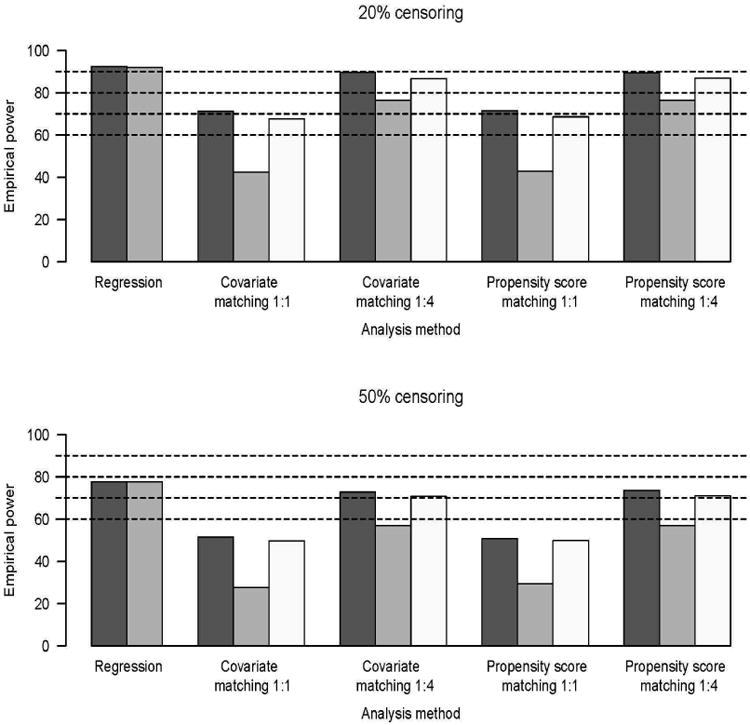
Empirical power; Usual Cox model, stratified Cox model, and marginal Cox model. Under 20% censoring, Cox regression model with all of the covariates applied to the entire cohort of patients had more than 90% power to detect existing treatment effect. In case of 1:1 matching, all methods applied to the matched cohort had 40-70% power to detect the treatment effect. Having 1:4 matching ratio resulted in power estimates slightly below those demonstrated by the Cox model applied to the entire cohort. Higher censoring proportion leads to uniformly lower power in detecting the treatment effect.

These simulations show the power advantage of the regression technique in a situation where the regression model is correctly specified. We also considered a situation where the data is generated from a propensity score model, placing the regression technique at a potential disadvantage. The resulting estimates of the Type I error rates and power were very similar to those summarized above and thus are not presented here. It should be noted that in certain situations where the relationship between treatment assignment and patient characteristics is complex (e.g, it depends on the interaction between the covariates) regular Cox model with simple linear covariate combination may have an elevated Type I error rate. Our simulation experiments indicate that this can be remedied by including the propensity score as a covariate into the regression model. The latter approach has received wide consideration, ^8,9,10 and could be used to enrich Cox model after including other covariates of interest.

Example

The data used in this article is a subset of a larger hematopoietic cell transplantation study conducted at the CIBMTR¹¹. The goal of the study was to examine the effect of having fungal infection prior to the transplantation. Invasive fungal infections historically are associated with a higher mortality rate among patients undergoing hematopoietic cell transplantation. For the sake of this presentation, 1,238 patients who were diagnosed with acute myeloid leukemia (AML) and underwent HCT between 2007 and 2009 involving an unrelated donor are considered. Among these patients, 127 were known to have an infection prior to the transplant and 1,111 of them were infection free. The analyses presented here are only for illustration of the statistical methodology. The results from our analyses should not be taken as a clinical conclusion.

We will focus on comparing survival in patients who have undergone transplant with known fungal infection to their counterparts without the infection. In order to eliminate possible differences with respect to various disease and transplant characteristics, analysis is adjusted for age, Karnofsky performance score, and disease stage. Sample characteristics are presented in Table 1.

Table 1. Characteristics of the HCT study sample.

		Infection
Characteristic	Value	Yes (N=127)	No (N=1,111)
Karnofsky performance score	<90	45 (35%)	372 (33%)
	≥90	82 (65%)	739 (67%)
Disease stage	Early	65 (51%)	581 (52%)
	Intermediate	28 (22%)	266 (24%)
	Advanced	34 (27%)	264 (24%)
Age	<40 years	40 (32%)	321 (29%)
	≥40 years	87 (68%)	790 (71%)

Models considered in the previous sections were applied to this data set. Results are summarized in Table 2. The results obtained by using Cox model applied to the entire study cohort of 1,238 patients indicate a significant difference in death rates between the patients who had an infection and those who did not have an infection prior to the transplant (p=0.0178). The hazard ratio estimates indicate that the risk of death is about 1.3 times higher among patients with infection as compared to those without it (HR=1.33, 95% confidence interval (1.05-1.68)).

Table 2. Results for the test for treatment effect in the HCT study.

	Matching #1		Matching #2
Analysis	HR (95% CI)	p-value	HR (95% CI)	p-value
Cox model; all covariates (n=1238)	1.33 (1.05-1.68)	0.0178	1.33 (1.05-1.68)	0.0178
Stratified Cox model (n=1238)	1.32 (1.04-1.67)	0.0207	1.32 (1.04-1.67)	0.0207
Covariate matching 1:1 (n=254)
Cox model	1.43 (1.02-1.99)	0.0357	1.09 (0.80-1.49)	0.5765
Stratified Cox model*	1.55 (1.03-2.33)	0.0344	1.22 (0.82-1.80)	0.3229
Marginal Cox model	1.43 (1.04-1.96)	0.0274	1.15 (0.86-1.53)	0.3573
Covariate matching 1:4 (n=635)
Cox model	1.38 (1.07-1.78)	0.0110	1.23 (0.96-1.58)	0.1002
Stratified Cox model	1.45 (1.10-1.92)	0.0080	1.42 (1.08-1.87)	0.0122
Marginal Cox model	1.42 (1.09-1.85)	0.0091	1.27 (0.99-1.63)	0.0545
Propensity score matching 1:1 (n=254)
Cox model	1.44 (1.03-1.99)	0.0286	1.31 (1.04-1.80)	0.1058
Stratified Cox model	1.68 (1.11-2.52)	0.0130	1.88 (1.24-2.85)	0.0029
Marginal Cox model	1.48 (1.08-2.03)	0.0138	1.37 (1.00-1.88)	0.0485
Propensity score matching 1:4 (n=635)
Cox model	1.25 (0.97-1.60)	0.0834	1.34 (1.04-1.72)	0.0209
Stratified Cox model	1.31 (0.99-1.73)	0.0601	1.46 (1.10-1.92)	0.0076
Marginal Cox model	1.28 (1.00-1.65)	0.0504	1.37 (1.08-1.75)	0.0106

^*All stratified and marginal Cox models are fitted with the main (treatment) effect only;

As seen from Table 2, matching techniques may lead to different results. In case of 1:1 and 1:4 matching -both based on covariate values themselves or the propensity score - the resulting sample included 254 and 635 subjects, respectively. It should be noted that, in the case of matching, selection of an untreated control (a patient without a pre-transplant fungal infection) involves some randomness. Therefore, regardless of the matching mechanism, results from a given matched data set may be different from those obtained if the matching procedure is to be repeated and a different set of controls is to be selected.

This phenomenon is illustrated by presenting results obtained by matching patients with and without fungal infection in the cohort twice (columns Matching #1 and Matching #2 in Table 1). In addition, note that different matching proportions and analysis techniques may lead to different conclusions. For example, marginal Cox model applied to the data set resulting from Matching #1 when patients with fungal infection were matched on the values of the covariates to those without it at the ratio 1:4 will yield the p-value of 0.0091 showing a significant difference in mortality between the two groups. When 1:4 matching was implemented via propensity scores, the resulting p-value from the marginal Cox model was 0.0504. However, repeating the 1:4 matching procedure (column Matching #2) with the marginal Cox model after covariate-based matching yields the p-value of 0.0545 and that after the propensity score matching is 0.0106.

Discussion

In many medical studies with the aim of assessing treatment effect or comparing groups of patients, several approaches could be employed. Often baseline characteristics of the patients may be imbalanced between the groups and adjustments need to be made to the design or analysis. This can be accomplished either via appropriate regression modeling or, alternatively, by conducting a matched pairs study. In this article, we looked at these two options in terms of their ability to detect a treatment effect in time-to-event studies. It is sometimes believed that a matched study will produce balanced groups where patients in the two groups being compared differ with respect to the treatment received but are similar regarding other characteristics. In survival analysis studies, matching is usually followed by a stratified or marginal Cox model which accounts for dependence between subjects within a pair or cluster. While matching aims to reduce bias it may suffer from loss of efficiency which results from restricting the analysis to a subset of patients. This issue can be especially notable if the matching ratio is low. Some other problems associated with matched studies have been pointed out in the literature. For example, Greenland and Morgenstern¹² showed that matching does not always increase efficiency in cohort studies for risk-difference and risk-ratio estimation. The value of matching in case-control studies has been discussed by many, and numerous publications indicate that such an approach is not always beneficial¹³. While in rare instances a balance achieved in the covariate distribution may decrease the variance of the estimators^14,15, discarding observations in the matching process will typically result in smaller sample sizes and may lead to increased variance which will obscure existing differences between groups. There is a body of research devoted to improving matching and estimation quality in matched studies under specific conditions (excellent overview and extensive reference list is provided by Stuart¹⁶). However, matched studies followed by simple unadjusted analysis are very common and frequently chosen instead of more flexible regression models. Our investigation shows that a Cox regression model applied to the entire cohort is often a more powerful tool in detecting a treatment effect.

Since matched studies result in a smaller sample size which can lead to reduced power, if possible, an investigator should strive to find a larger number of untreated controls for each treated subject. A greater matching ratio mitigates much of the power loss associated with the sample size reduction occurring in matched studies. Furthermore, results from a given matched data set may be different from those obtained if the matching procedure was to be repeated and a different set of controls was to be selected, illustrating the variability inherent in the study design. Selecting a matched study design may be justified when there is a need to reduce the number of individuals when extensive additional data collection on everybody in the final data set needs to be done. Another instance when a matched study may be desired is when there is a large degree of heterogeneity among cases (for example, specific disease diagnosis ranges widely) and regression model accounting for that would be very complicated and, given smaller sample sizes even impossible to fit. In most other cases, a Cox regression model applied to the entire study cohort can effectively address confounding attributable to observed covariates and maximizes power by using all the data available. Despite imbalance in patient characteristics by treatment when using the full cohort of patients, the Cox regression model can often produce good estimates of the treatment effect unless the imbalance is very severe. However, utmost care is needed with the Cox regression model to adequately capture the relationship between the covariates and the outcome and provide a proper adjustment for these covariates. An ability to build an adequate regression model for survival data depends not only on the number of subjects in the study but also on the number of observed events. Thus planning a treatment comparison involving time to event censored data requires careful assessment which will depend on a number of factors such as initial number of patients eligible for the study, the rate at which the event of interest is occurring, the length of the follow-up period, and number of the covariates to be investigated¹⁷. It also includes assessment of the proportional hazards assumption (that the effect of a covariate on the hazard rate is the same at each time point), checking for interactions between patient characteristics and including important ones in the model, assessing the functional form of the relationship between quantitative covariates (e.g. age) and outcome, and ensuring sufficient overlap of patient characteristics to allow for a proper risk adjustment. Other researchers have proposed using the propensity score as a covariate in a regression model utilizing the entire study population, to help minimize bias due to confounding.^8,9,10 Our simulation studies indicate that such an approach works well in a variety of situations. Complying with assumptions and conditions to ensure the adequacy of the analysis and conclusions that follow are not only pertinent to regression modeling. There are many pitfalls in the matching process and analysis that may affect their feasibility and performance as well^1,10,13,16. A well chosen Cox regression model has the advantage over matched studies of using all patient information available leading to increased efficiency.

Highlights.

• Accounting for imbalances in patient characteristics is needed when assessing treatment effect.

• Choices in study design: (1) regression modeling or (2) matched pairs study.

• Regression model is often a more powerful tool in detecting treatment effect than a matched study.

Appendix.

Methods

In a cohort of patients assessed for time to a particular event, the data consists of a follow-up time recorded for each study participant along with an event indicator telling the investigator whether the patient experienced the event. For every subject, a set of covariates, Z, is available. The Cox model is concerned with the hazard rate h(t) which represents the rate at which individuals who are still at risk fail at time t. The Cox model can be written as follows:

$$\mathrm{h}(\mathrm{t}|\mathrm{Z})={\mathrm{h}}_0(\mathrm{t})\mathrm{\text{exp}}(\beta \mathrm{Z}),$$

where β are regression coefficients and h₀(t) is an unspecified baseline hazard function which is common to all patients. The baseline hazard function h₀(t) quantifies the rate of failure among “baseline” or “reference” individuals with covariate value Z=0. Note that if we look at two individuals with covariate values Z=l and Z=0, i.e. Z is treatment assignment indicator (Z=l for those in treatment group and Z=0 for patients receiving placebo), their hazard ratio of experiencing the event is

$$\frac{h(t|Z=1)}{h(t|Z=0)}=\frac{\mathrm{h}0(\mathrm{t})\exp (\mathrm{\beta }\times 1)}{\mathrm{h}0(\mathrm{t})\exp (\mathrm{\beta }\times 0)}=\exp (\mathrm{\beta }),$$

which is constant. The quantity exp(β) can be interpreted as the risk of experiencing the event if the individual was in treatment group relative to the risk of having the event among those individuals receiving placebo. The stratified Cox model used in analyzed paired data relies on the hazard function introduced earlier but assumes a separate baseline hazard function for each pair k:

$$\mathrm{h}(\mathrm{t}|\mathrm{Z})={\mathrm{h}}_{0\mathrm{k}}(\mathrm{t})\exp (\mathrm{\beta }\mathrm{Z}),\mathrm{k}=1,\dots ,\mathrm{K}.$$

This model assumes a common treatment effect or, equivalently, hazard ratio across all pairs while the baseline hazards in each pair can be different. In this case, the quantity exp(β) can be interpreted as the risk of experiencing the event if the individual received the treatment (Z=l) relative to the risk of having the event for the individual from the same pair who received the placebo (Z=0). Inference for the regression coefficients β is based on a within pair treatment effect. When there is censoring present, only pairs where the smaller of the two times is an event time contribute information about the hazard ratio thus the effective sample size may be rather small.

Simulation study design

The survival data is generated in the following manner. First, we generate covariate values for 100 treated cases and 1000 untreated controls. Three binary (0/1) covariates are being considered:

• Treatment indicator Z₁=1 for cases, 0 for controls;

• Z₂=1 for 40% of cases and 70% of controls;

• Z₃=1 for 50% of cases and controls.

After the covariate values are obtained, the survival time for each subject is generated from the Cox model where all of the covariates satisfy the proportional hazards assumption:

$$\mathrm{h}(\mathrm{t}|{\mathrm{Z}}_1,{\mathrm{Z}}_2,{\mathrm{Z}}_3)={\mathrm{h}}_0(\mathrm{t})\exp ({\mathrm{\beta }}_1{\mathrm{Z}}_1+{\mathrm{\beta }}_2{\mathrm{Z}}_2+{\mathrm{\beta }}_3{\mathrm{Z}}_3).$$ (1)

Here, the covariate set for a given individual is (Z₁, Z₂, Z₃) with Z₁ being the group (treatment) indicator. Regression coefficients (β₁, β₂, β₃) are estimated based on the observed data. When the goal is to evaluate the impact of various study design options in the context of hypothesis testing for a treatment effect, the focus is on testing the hypothesis H₀: β₁=0 vs Ha: β₁≠ 0. Type I error rate of the test is assessed by generating the data where there is no difference between the two groups and thus the data is simulated from model (1) with β₁=0. In order to evaluate the power of the test the data was generated from the same model with β₁=0.4 which corresponds to treated subjects having 1.5 times higher risk of experiencing the event as compared to the untreated controls. Other quantities in generating the data from model (1) were as follows: β₂=0.5, β₃= -0.5, h₀(t)=1. In order to assess the impact of censoring, 20% and 50% censoring rates were considered.

References

- 1.Rosenbaum PR, Rubin DB. The central role of the propensity score in observational studies for causal effects. Biometrika. 1983;70:41–55. [Google Scholar]
- 2.Le-Rademacher J, Brazauskas R. In: Inference for paired survival data Handbook of Survival Analysis. Klein JP, van Houwelingen HC, Ibrahim JG, Scheike TH, editors. CRC Press; 2013. pp. 615–632. [Google Scholar]
- 3.Wei LJ. The accelerated failure time model: A useful alternative to the Cox regression model in survival analysis. Statistics in Medicine. 1992;11:1871–1879. doi: 10.1002/sim.4780111409. [DOI] [PubMed] [Google Scholar]
- 4.Klein JP, Moeschberger ML. Survival Analysis: Statistical Methods for Censored and Truncated Data. 2nd. Springer-Verlag; New York: 2003. [Google Scholar]
- 5.Glidden DV, Vittinghoff E. Modelling clustered survival data from multicentre clinical trials. Statistics in Medicine. 2014;23:369–388. doi: 10.1002/sim.1599. [DOI] [PubMed] [Google Scholar]
- 6.Lee EW, Wei LJ, Amato DA. Cox-type regression analysis for large number of small groups of correlated failure time observations. In: Klein JP, Goel PK, editors. Survival Analysis: State of the Art. 1992. [Google Scholar]
- 7.Ho D, Imai K, King G, Stuart E. MatchIt: Nonparametric Preprocessing for Parametric Causal Inference. Journal of Statistical Software. 2011;42(8):1–28. [Google Scholar]
- 8.D'Agostino RB. Tutorial in Biostatistics. Propensity score methods for bias reduction in the comparison of a treatment to a non-randomized control group. Statistics in Medicine. 1998;17:2265–2281. doi: 10.1002/(sici)1097-0258(19981015)17:19<2265::aid-sim918>3.0.co;2-b. [DOI] [PubMed] [Google Scholar]
- 9.Austin PC. The performance of different propensity score methods for estimating marginal hazard ratios. Statistics in Medicine. 2013;32:2837–2849. doi: 10.1002/sim.5705. [DOI] [PMC free article] [PubMed] [Google Scholar]
- 10.Beal SJ, Kupzyk KA. An introduction to propensity scores: What, when, and how. Journal of Early Adolescence. 2014;34(1):66–92. [Google Scholar]
- 11.Maziarz RT, McLeod A, Chen M, et al. Outcomes of allogeneic HSCT for patients with hematologic malignancies (AML, ALL, MDS, CML) with and without pre-existing fungal infections; A CIBMTR study. Biology of Blood and Marrow Transplant. 2013;19(2) 1:S124–S125. [Google Scholar]
- 12.Greenland S, Morgenstern H. Matching and efficiency in cohort studies. American Journal of Epidemiology. 1990;131:151–159. doi: 10.1093/oxfordjournals.aje.a115469. [DOI] [PubMed] [Google Scholar]
- 13.Rose S, Van der Laan MJ. Why match? Investigating matched case-control study designs with causal effect estimation. The international Journal of Biostatistics. 2009;5(1) doi: 10.2202/1557-4679.1127. Article 1. [DOI] [PMC free article] [PubMed] [Google Scholar]
- 14.Snedecor GW, Cochran WG. Statistical Methods. 7th. Iowa State University Press; Ames, IA: 1980. MR0614143. [Google Scholar]
- 15.Smith H. Matching with multiple controls to estimate treatment effects in observational studies. Sociological Methodology. 1997;27:325–353. [Google Scholar]
- 16.Stuart EA. Matching methods for causal inference: A review and a look forward. Statistical Science. 2010;25(1):1–21. doi: 10.1214/09-STS313. [DOI] [PMC free article] [PubMed] [Google Scholar]
- 17.Vittinghoff E, McCulloch CE. Relaxing the Rule of Ten Events per Variable in Logistic and Cox Regression. American Journal of Epidemiology. 2007;165(6):710–718. doi: 10.1093/aje/kwk052. [DOI] [PubMed] [Google Scholar]