Enhancer scanning to locate regulatory regions in genomic loci

Abstract

The present protocol provides a rapid, streamlined and scalable strategy to systematically scan genomic regions for the presence of transcriptional regulatory regions active in a specific cell type. It creates genomic tiles spanning a region of interest that are subsequently cloned by recombination into a luciferase reporter vector containing the Simian Virus 40 promoter. Tiling clones are transfected into specific cell types to test for the presence of transcriptional regulatory regions. The protocol includes testing of different SNP (single nucleotide polymorphism) alleles to determine their effect on regulatory activity. This procedure provides a systematic framework to identify candidate functional SNPs within a locus during functional analysis of genome-wide association studies. This protocol adapts and combines previous well-established molecular biology methods to provide a streamlined strategy, based on automated primer design and recombinational cloning to rapidly go from a genomic locus to a set of candidate functional SNPs in eight weeks.

Introduction

Developing tools for analysis of GWAS loci

Genome-wide association studies (GWAS) have been extremely successful in identifying a large number of predisposition loci for a series of human diseases and conditions including cancer ^1,2. These risk loci are physical locations defined by tagging SNPs associated with risk but for which the mechanism underlying susceptibility is generally unknown. It is normally hypothesized that susceptibility is conferred by genetic variation, represented by the tagging SNP or by those in linkage disequilibrium (LD) with it, with a functional impact on coding or non-coding elements of the genome ^3,4.

Typically, functional analysis starts by identifying a comprehensive set of candidate functional SNPs operating in the locus. It then proceeds by applying progressively stringent criteria to discard variants that do not contribute functionally and are unlikely to be driving association with risk. The identification of functional SNPs allows the generation of several testable hypotheses on how different alleles might functionally contribute to cancer risk ⁵. Functional SNPs might occur in coding regions, in which case the determination of the target gene is straight forward (i.e. the gene in which the coding SNP is located) ⁶. Next, these coding SNPs are assessed for the impact of different alleles on protein stability and function. However, the overwhelming majority of cancer susceptibility loci identified by GWAS is located in non-coding regions ⁷.

In these cases, the principal hypothesis is that the functional SNPs modify the activity of transcriptional regulatory regions, such as enhancers, that interact with the promoter(s) of target gene(s) ³. Thus, in these cases it is critical to identify regulatory regions whose activity might be modulated by different SNP alleles and subsequently define which gene(s) are affected by the regulatory region.

Despite the rapid progress in cancer risk loci identification by GWAS ^8,9 the determination of the functional mechanisms underlining risk for a large number of loci has proceeded more slowly due, at least in part, to a lack of systematic assays to rapidly evaluate all SNPs present in genomic region of interest for regulatory activity. The protocol described here is designed to fill this gap.

To comprehensively capture the initial set of candidate functional SNPs to be tested it is acceptable to sacrifice specificity to obtain higher sensitivity. This initial step should capture most true positive signals. Then, downstream analysis using stringent criteria (e.g. that they show allele specific effects in vitro and in vivo) will progressively eliminate false positive signals. Assays based on naked (or non-chromatinized) DNA such as electrophoretic mobility shift assays (EMSAs) or luciferase reporter assays are particularly suited for this step as they will identify any putative active sequence in the underlining DNA provided that the required factors are expressed in the cell of interest ¹⁰.

To accelerate discovery and functional analysis of GWAS loci we developed a streamlined method that can systematically scan for regions with regulatory activity in a cell line of choice and can be scaled-up to study relatively large genomic regions (100-500 kb). The method takes advantage of online bioinformatics tools and combines a polymerase chain reaction (PCR)-based generation of tiling clones spanning the region with high efficiency recombination cloning. This method has been used successfully in the analysis of ovarian ¹¹, brain ¹², and breast (GMF unpublished data) cancer predisposition loci.

Applications of the method

Recently, a large scale effort to identify regulatory regions in the human genome was conducted by the ENCODE (Encyclopedia of DNA Elements) consortium and a comprehensive landscape of chromatin modifications and states is now available for several cell lines ^13-18. A similar effort was also undertaken by the FANTOM (Functional Annotation of the Mammalian Genome) consortium ^19,20. Data from these initiatives can be used to identify SNPs that overlap with chromatin features and are more likely to be functional. In this case, our method can provide additional validation as well as a means to test whether different alleles of the SNP may lead to changes in activity.

In addition, since regulatory region activity may depend on the presence of cell-type specific transcription factors or certain stimuli ¹⁵, ENCODE data may not be available for specific cell types and conditions relevant to the investigator's experimental question. For example, a significant number of cell types in ENCODE are cancer cell lines but ideally, analysis of loci implicated in predisposition should be performed in the normal cell from the tissue of origin of the cancer being studied ³. Thus, our method can be applied to primary (or immortalized) normal cell lines to complement or add to ENCODE data.

In some cases, SNPs located in a coding region might also have a simultaneous effect on a regulatory motif ²¹. These coding regions can also be tested in our method for regulatory activity. Finally, although the method is primarily geared to analyze germ line variants, it can be applied to perform functional analysis of variants found in non-coding regions derived from whole genome or targeted clinical sequencing efforts of tumor DNA ²².

Alternative Methods

Two recently published methods, Massively Parallel Reporter Assay (MPRA) and STARR-Seq, are also designed to identify regions of regulatory activity ^23,24. MPRA, STARR-Seq, and the method presented here measure regulatory activity in a non-chromatinized plasmid-based DNA template and require a cell host with high transfection efficiency. MPRA and STARR-Seq are based on libraries of synthesized oligonucleotides or Bacterial artificial Chromosome fragments, respectively. While both MPRA and STARR-Seq can interrogate a much larger number of candidate regulatory segments per experiment than our method, they also require the generation of high complexity representative libraries involving several additional steps of quality control ^23,24. Currently, high complexity representative libraries of mammalian genomes are limited to six BACs in STARR-Seq ²⁴. In combination with sequencing data analysis required to identify regulatory segments, MPRA and STARR-Seq require more experienced investigators and significantly more time for optimization. MPRA is designed to test the activity of relatively short sequences (87 nt)²³ and while ideal to identify optimal sequences for specific transcription binding sites, it may be unable to detect regulatory activity from longer sequences that depend on cooperative binding of different transcription factors. Thus, we believe that our method provides an alternative to investigators that are conducting an analysis focusing on one or a few loci. Investigators looking to perform analysis of multiple genomic loci are encouraged to compare MPRA, STARR-Seq, and Enhancer Scanning to decide which method is more appropriate for their project scope, level of experience, and resources.

Limitations

The enhancer scanning method presented here is based on the use of a plasmid-based reporter gene to detect regions in the genomic DNA with transcriptional regulatory activity. As other naked DNA-based assays (such as EMSAs) it identifies sequences present in the DNA that have the ability to recruit and bind transcriptional regulators. It is conceivable that the underlining DNA (exposed in the plasmid-based assay) that carries the activity may, in certain chromatin contexts, be hidden by tight nucleosome packing, repressive chromatin features and DNA methylation. Thus, some tiles may be false positive hits. Additionally, some amplicons with repeats may be especially difficult or impossible to amplify and therefore may not be able to be tested using this method.

Although we have identified tiles with repressive activity (i.e. display a fold reduction in relation to the negative empty vector control) we have not characterized these in detail to determine whether they represent true repressive regions as many of them do not co-localize with ENCODE chromatin features suggestive of repression, such as CTCF ChIP-Seq (Chromatin Immunoprecipitation followed by Sequencing) peaks. Thus, further work is needed to determine whether this method is appropriate to identify repressive regions.

The sensitivity of the method presented here is dependent on transfection efficiency and cells that are difficult to transfect, or experiments in which transfection is sub optimal, may not identify all tiles with activity. Use of a set of internal controls greatly minimizes false negatives due to transfection failures. The ability of the enhancer to activate transcription of a cognate promoter region depends of the formation of an adequate DNA loop between the enhancer and promoter ²⁵. Thus, it is conceivable that even when testing both cloning orientations in a plasmid context, an optimal loop may not form between the region and the promoter leading to false-negative results. To estimate the fraction of false-negatives, in the absence of well characterized region to use as benchmark, we determined the number of active enhancers as defined by ENCODE biofeatures that failed to be positive in the Enhancer Scanning method. In our experience approximately 15% of tiles predicted by ENCODE Biofeatures failed to show activity in Enhancer Scanning (a similar fraction was found using STARR-Seq, not shown). However, this number may not necessarily reflect false-negative regions because cells chosen for enhancer scanning were not the exact same cell type used to obtain ENCODE biofeatures. Moreover, some regulatory regions may be dynamic and shift from active to inactive during cell culture.

Finally, it is unclear to what extent the detection of a regulatory activity using a heterologous promoter affects the results. Although most enhancers function with any promoter¹⁰ some enhancer-promoter interaction depends on binding factors or other promoter features (biochemical compatibility) ²⁶. Thus, in the case of post-GWAS studies, where several promoters in the region might be potential targets, we suggest using the viral promoter for the first screen and once the target gene is identified (by expression Quantitative Trait Loci, eQTL analysis or Chromosome conformation capture techniques) a tile can be tested again with the desired promoter.

Experimental Design

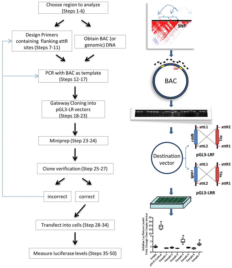
The complete procedure is depicted in Figs. 1 and 2. Essentially, we start with a genomic region identified by a GWAS as associated with risk for a certain condition (Fig. 2A) and we assume that the tagging SNP may not necessarily represent the functional SNP. Next, in order to capture the variation in the locus we can use LD structure information and retrieve all SNPs in (LD) with the tagging SNP (Fig. 2B; Procedure Steps 1-6) ^27,28. As a rule of thumb, we retrieve sets of SNPs in LD in 1000 Genomes Project with r² ≥ 0.2, ≥0.5, or ≥0.8. These thresholds are arbitrary and serve as a guideline for the investigator to decide which set to pursue further analysis appropriate for the resources and time available.

Figure 1. General overview of the Enhancer Scanning method.

Map for pGL3-Promoter is from Promega.

Figure 2. Strategies to analyze regions containing candidate functional SNPs.

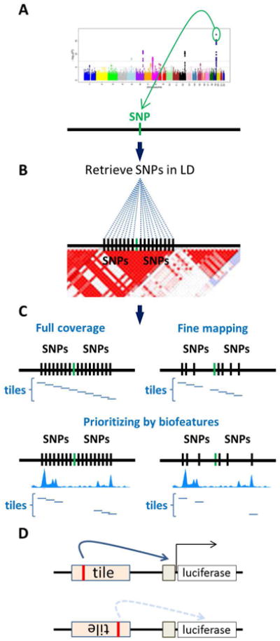
A. A genomic region identified by a GWAS as associated with risk for a certain condition. B. Retrieval of SNPs in linkage disequilibrium with the tagging SNP. C. Tiles can be created to interrogate all regions containing SNPs, or if fine mapping data is available only a select number of tiles containing the SNPs most likely to be associated with the trait need to be analyzed. Tiles can be further prioritized depending on whether they overlap with chromatin features indicative of regulatory activity. D. To increase the chances to identify a regulatory region tiles are tested in both orientations in regard to the promoter. Manhattan plot in the figure is adapted from (PLoS Genet. 2010 Oct 28;6(10):e1001184).

When fine mapping data is available (Fig. 2C) investigators may want to identify the region that contains all the statistically significant SNPs. Alternatively, prioritizing SNPs with a likelihood ratio (SNP relative to the top signal SNP) of >1:100 (or >1:1000) can reduce the number of SNPs to be analyzed ²⁹. The region of interest is delimited by the most telomeric and the most centromeric SNPs flanking the set (Fig. 2C).

With the region of interest defined we generate tiles by PCR spanning the whole region with each tile of approximately 2 Kb (Fig. 2C; Procedure Steps 7-11). This size is a compromise between having to generate the least amount of tiles to cover a region and efficient and reproducible PCR amplification. Regions with repetitive sequences may need smaller tiles to facilitate amplification. The PCR primers used are designed to include attL sequences to mediate recombinational cloning into destination vectors, pGL3-LRF and pGL3LRR (Fig. 3), which contain a luciferase gene driven by a basal promoter (Fig. 1). We converted the pGL3-Promoter vector (Promega) to a Gateway^® destination vector by inserting a blunt-ended cassette of the ccdB gene and the chloramphenicol resistance gene flanked by attR1 (5′-ACAAGTTTGTACAAAAAAGCTGAAC-3′) and attR2 (5′-GACCACTTTGTACAAGAAAGCTGAAC-3′) sites into a SmaI site of pGL3-Promoter vector (Fig. 3). Two recombinant vectors, carrying the cassette in each orientation, pGL3-LRF and pGL3-LRR, are then used to clone individual tiling clones by recombination (Procedure Steps 12-27). Plasmids containing tiling clones in both orientations are then transfected in an appropriate cell type and activity of luciferase is measured and compared with the corresponding pGL3-LR destination vector (Fig. 1, bottom right) (Procedure Steps 28-50). Alternatively, inserting a tile into the pGL3-Promoter vector can be done by conventional cloning using restriction digest and ligation (Procedure Step 10). In this case, PCR primers used to amplify each tile should contain the desired restriction site present in the multiple cloning site (KpnI, SacI, MluI, NheI, XhoI, BglII) (Procedure Step 10).

Figure 3. Vector maps.

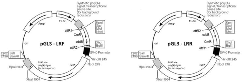
Maps for pGL3-LRR and LRF are adapted from the original map of the backbone PGL3-Promoter from Promega. Luc+, luciferase gene; ori, origin of replication; Amp^r, ampicillin resistance gene; f1 ori, f1 phage origin of replication; attR1 (5′-ACAAGTTTGTACAAAAAAGCTGAAC-3′) and attR2 (5′-GACCACTTTGTACAAGAAAGCTGAAC-3′); CmR, chloramphenicol resistance gene; cddB, gene coding for a DNA gyrase lethal to E. coli.

To be considered a candidate functional SNP, we expect tiles containing different alleles to show statistically significant differences (p ≤ 0.05) in reporter activation. If the method is used to validate regions suggested by analysis of ChIP-Seq or FAIRE-Seq (Formaldehyde-Assisted Isolation of Regulatory Elements) data a complete tiling of the whole region is not necessary and only tiles overlapping desired features can be generated greatly reducing the number of tiles to test (Fig. 2C). Tools such as RegulomeDB and FunciSNP can identify which SNPs overlap with data from ENCODE or other sources ^30,31. Here we use the classic operational definition of transcriptional enhancer as “discrete DNA elements that contain specific sequence motifs with which DNA-binding proteins interact and transmit molecular signals to genes”³². ENCODE data show that chromatin features of enhancers are that they are located in DNAse I hypersensitive regions that contain high levels of H3K4me1 (Histone H3 Lysine 4 mono-methylation) in relation to H3K4me3 (tri-methylation)^15,33. Although enhancers are expected to operate independent of orientation and position relative to the target promoter ³⁴, because the relative position of the binding site in relation to the promoter of the reporter may influence expression, tiles should be tested in both cloning orientations (Fig. 2D).

True functional SNPs are also expected to show allele specific differences in enhancer activity. Risk alleles may create or disrupt a specific binding site and it is recommended to test both alleles for each SNP. Different alleles can be introduced in the tiles using Quick Change PCR mutagenesis ³⁵ (Procedure Steps 51-53). Sanger sequencing, using universal primers RVprimer3 and GLprimer2 (Promega), is recommended to verify the variant after mutagenesis. Additional primers may be necessary to cover the entire region and should be designed approximately 100 bp from the start of region to be sequenced.

Choice of template, tile verification, and host cell

Once the region of interest is defined we generate tiles by PCR using human genomic DNA or a Bacterial Artificial Chromosome (BAC) clone containing the region of interest (Fig. 1). In our experience the latter provides a more robust option to amplify the tiles. It is expected that the BAC is likely to contain the major allele for the SNPs, but could represent the minor allele. In addition, depending on the number of loci being studied and the size of regions to be analyzed there could be hundreds of tiling clones to be processed simultaneously increasing the chance of sample mix-ups. Thus, it is useful to sequence a sample (or all) of the clones to confirm their identity and to determine the correct allele being tested.

Ideally the host cell for the transfection should represent a tissue compartment relevant for the disease under study. For example, cells from normal intestinal crypts when studying colorectal cancer. However, primary cells might be difficult to transfect and immortalized or cancer cells may provide an alternative, but the use of these cells lines should be kept in mind when interpreting the results.

Controls

Several controls are advisable to guarantee data quality and wise use of resources and reagents. We found that because in each experiment a large number of luciferase measurements are going to be made, it is important to have a monitor of whether the transfection has worked before processing samples. We recommend the use of a parallel transfection with a green fluorescent protein (GFP) expression vector of choice and when there are no detectable GFP-positive cells we do not proceed to lyse cells and measure luciferase. We also include a positive control (pGL3-Control Vector containing with a SV40 enhancer) and expect its activity to be consistent across transfections (10-20× the negative control in the experiment, for example). Eight technical replicates are performed for each tile in each orientation and luciferase readings are averaged and compared to the negative control. The negative controls used are the plasmids that only include the recombination cassette in both orientations and are compared to the tested tiles of the same orientation. An additional control derived from the region being studied is also recommended and can be designed by identifying a region with no candidate SNPs and with no chromatin markers indicative of activity. We recommend the inclusion of all controls in every plate. As a rule of thumb we perform at least two independent experiments typically done on different days (biological replicates) and only tiles that have significant activity in both biological replicates are considered for further analysis.

As the goal is the identification of functional SNPs, confirmation by sequencing of the desired clone is an absolute requirement. Even when starting from a template of known genotype (BAC or a genotyped cell line genomic DNA) and using a proof-reading polymerase cross-contamination is possible as are very rare PCR errors. When starting from a genomic DNA template of unknown genotype or using non-proof reading polymerase we recommend sequencing all clones which might add to cost and should be taken into consideration when deciding which polymerase to use.

Statistical analysis

Results from transfections with individual tiles are analyzed in eight replicates. This number allows for the generation of box whisker plots and maximizes the 96-well setup but investigators might want to scale it down to reduce costs. Raw readings from firefly (Photinus pyralis) luciferase are normalized against an internal Renilla reniformis luciferase control driven by a minimal promoter, pRL-TK (Renilla luciferase driven by thymidine kinase promoter) to adjust for differences in transfection efficiency in different wells. Next, we set the negative control (pGL3-LRF and pGL3-LRR empty vectors) as the reference and results are transformed to fold over the negative control. Statistical analysis is performed by comparing the exact means and p ≤ 0.05 is considered significant. When testing a large number of tiles, a multiple testing correction can be applied (for example, p≤ 0.05/number of tiles being tested). Alternatively, a less stringent false discovery rate can also be applied for prioritization. However, we feel that due to the stage of SNP analysis in which this assay is being performed it would be unwarranted to apply multiple testing corrections as true positive clones with small effects might be discarded. Additional more stringent tests are subsequently applied to the tiles (for example, allele-specific differences, activity in EMSA, etc.) to weed out false positive hits.

Materials

Reagents

• Bacterial artificial chromosomes (Life Technologies, or Empire Genomics)

• Cloning and sequencing Primers designed to cover the region of interest (Invitrogen™ or IDT custom oligonucleotides; can be synthesized at 25 nM scale, desalted; and can also be ordered in 96-well plate format)

• Sequencing primers: pGL3-Seq-Rev 5′-CCTCGGCCTCTGCATAAATA-3′ or pGLprimer2 (Promega) 5′-CTTTATGTTTTTGGCGTCTTCCA’-3′; RVprimer3 (Promega) 5′-CTAGCAAAATAGGCTGTCCC-3′; additional primers specific to the region may be required to cover the entire tile.

• Chloramphenicol (Sigma; cat.no. C0378)

• Ampicillin (Sigma; cat.no. A1593)

• LB broth (Sigma; cat.no. L3022-1KG)

• Agar-agar (EMD Chemicals; cat.no. 1.01614.100)

• 100 mm Bacterial plates (VWR Scientific; cat.no. 25384-008)

• HiSpeed^® Plasmid Maxi kit (Qiagen cat.no. 12663), or Plasmid Maxi Kit (Qiagen cat.no. 12163)

• Cell lines. The host cell used for the assays will be dependent on the investigator's choice (see Choice of template, tile verification, and host cell). ! CAUTION We recommend avoiding cell lines commonly misidentified or cross-contaminated (http://iclac.org/databases/cross-contaminations/). Cell lines should be regularly checked for authenticity (for example, using Short Tandem Repeat authentication) and for Mycoplasma contamination.

• Cell culture medium for the cell line of choice

• 100 mm tissue culture plates (Fisher; cat.no. 08-772-23)

• PureLink Genomic DNA Mini Kit (Life Technologies; cat.no. K1820-01)

• Hot Start Taq Polymerase kit (Qiagen; cat.no. 203205); for difficult tiles we recommend KAPA HiFi HotStart PCR kit (KAPA; cat.no. KK2501)

• dNTP Mix (Thermo Scientific; cat.no. R0242)

• DNA gel purification kit Qiaquick (Qiagen; cat.no. 28706)

• One Shot^® TOP10 Chemically competent E.coli (Life Technologies; cat.no. C4040-06)

• pGL3-Promoter vector (Promega; cat.no. E1761)

• pGL3-Control Vector (Promega; cat.no. E1741)

• pGL3-Enhancer vector (Promega; E1771)

• pGL3-LRF and pGL3-LRR (Monteiro Lab; available through Addgene # 66936 and 66937)

• pRL-TK Vector (Renilla luciferase internal control) (Promega; cat.no. E2241)

• pGFP (Clontech; cat.no. 632370)

• Gateway pDONR 221 vector (Life Technologies; cat.no. 12536-017)

• Gateway LR Clonase II Enzyme Mix (Life Technologies; cat.no. 11791-020)

• QuikChange II XL Site-Directed Mutagenesis Kit (Agilent Technologies; cat.no. 200521)

• XhoI and MluI restriction endonucleases (New England Biolabs; cat.no. R0146L and R0198L)

• Restriction endonuclease buffer NEB Buffer 3 (New England Biolabs; cat.no. B7003S)

• Bovine Serum Albumin 1× (New England Biolabs; cat.no. B9001S)

• S.O.C medium (Life Technologies; cat.no. 15544034)

• Glycerol (Sigma; cat.no. G5516)

• Agarose (Sigma; cat.no. A5093-500G)

• Electrophoresis buffer 1× TAE. Trimethylol Aminomethane, Tris (hydroxymethyl) aminomethane (Fisher Scientific; cat.no. BP152-5)

• Acetic Acid, Glacial (Fisher Scientific; cat.no BP2401-212) ! CAUTION Corrosive. Flammable liquid and vapor – keep away from open flame. Causes severe skin burns and eye damage – wear protective gloves and goggles.

• Ethylenediamine Tetraacetic Acid, Disodium Salt Dihydrate (Fisher Scientific; cat.no. BP120-500)

• Gel loading buffer 6× (New England BioLabs; cat.no. B7021S)

• Electrophoresis molecular weight markers Kb DNA ladder (Agilent; cat.no. 201115)

• DNA Miniprep kit (Qiagen; cat.no. 27106)

• TE buffer (Ambion; cat.no. AM9849)

• Proteinase K (Life Technologies; cat.no.255300 15)

• 14 ml polypropylene round bottom tubes for bacterial miniprep (Fisher; cat.no. 14-959-11B)

Transfection reagents

• Fugene6 (Promega; cat.no. E2691),

• Fugene HD (Promega; cat.no. E2311),

• Lipofectamine2000 (Life Technologies; cat.no. 11668-019), or Lipofectamine3000 (Life Technologies; cat.no. L3000-008).

  ▴ CRITICAL For Fugene reagents pipet transfection reagents directly into the medium and avoid touching the plastic walls of the tube. Chemical residues in plastic vials can significantly decrease the biological activity of the reagent.

• 96 well plates (Fisher; cat.no. 07-200-587)

• Dual-Glo^® luciferase reagents (Promega, catalog # E2980)

Equipment

• Computer with internet connection

• 37°C Incubator for bacteria

• 37°C Water bath

• 37°C shaker for bacterial culture

• 37°C CO₂ Incubator for tissue culture

• Inverted microscope

• Laminar flow hood for manipulating cells

• Thermocycler

• Plate-reader Luminometer (SpectraMaxL or equivalent)

Reagent Setup

PCR setup

In the following tables we provide a starting guide that can be adjusted according to the primers being used. We suggest starting with HotStarTaq polymerase PCR reaction due to its lower cost. For difficult to amplify tiles we recommend using the KAPA HiFi HotStart PCR reaction. Troubleshooting advice can be found in Table 1.

Table 1. Troubleshooting.

Step	Problem	Possible Reason	Possible Solution
12A	Low yield	Difficult to replicate or toxicity from BAC	Try different DNA prep kits to increase yield; culture a larger volume of bacterial culture; replace bacterial host
14	No amplicons	Difficult / repetitive regions, poor primer design	Repeat the reaction using Kappa HiFi PCR kit. This polymerase is significantly more expensive and may be prohibitive to amplify all tiles in a large scale experiment. PCR reactions using genomic DNA as template are also more difficult and we recommend when possible to use BAC DNA as template, which also avoids specificity problems (other non-relevant regions in the genome being primed). Gradient PCR may also improve the PCR reaction. If all fail, redesign the primers shifting their position.
14	Multiple bands	Mispriming by PCR primers; presence of a repetitive region	Optimize PCR reaction by increasing annealing temperature. Attempt to isolate the band with the expected size by gel electrophoresis and confirm by sequencing
22	No clones	att regions might have been incorrectly designed, longer (>5kb) tile	See troubleshooting section by Life Technologies (https://www.lifetechnologies.com/us/en/home/technical-resources/technical-reference-library/cloning-technical-support-center/recombination-based-cloning/recombination-based-cloning-troubleshooting.html)
34	Failed to show GFP positive cells (do not proceed with measuring luciferase)	Poor transfection efficiency	Optimize transfection conditions by varying the number of cells and transfection reagents. Verify that transfection reagents are not too old or have been frozen and thawed multiple times. If problem persists check cells for mycoplasma or choose an alternative cell line.

! CAUTION Use of a non-proof reading polymerase may lead to the introduction of sequencing errors in some clones. While most will not be significant (do not modify the candidate SNPs or a binding sequence neighboring the SNPs), a few may create false positives or false negatives.

HotStarTaq PCR Reaction Mix
Reagent	Initial Conc.	Final Conc.	Vol.
PCR Buffer (X)	10	1	5
dNTP (mM)	2	0.2	5
Primer Forward (pMoles/μl)	20	0.4	1
Primer Reverse (pMoles/μl)	20	0.4	1
HotStarTaq pol (U/μl)	5	0.25	0.25
BAC (ng/μl)	50	2	2
H2O			35.75
Total Vol. (μl)			50
HotStarTaq PCR conditions
Step	Temp (°C)	Time	Cycles
Denaturation	95	15 min	1
Denaturation	94	1 min
Annealing	55	1 min	30
Extension	72	60sec/kb
Final extension	72	10 min	1

KAPA HiFi HotStart PCR Reaction Mix
Reagent	Initial Conc.	Final Conc.	Vol.
2× KAPA HiFi HotStart Ready Mix	2	1	12.5
Primer Forward (pMoles/μl)	10	0.4	1
Primer Reverse (pMoles/μl)	10	0.4	1
BAC (ng/μl)	50	2	2
H2O			8.5
Total Vol. (μl)			25
KAPA HiFi HotStart PCR conditions
Step	Temp (°C)	Time	Cycles
Denaturation	95	3 min	1
Denaturation	98	20 sec
Annealing	65	15 sec	25
Extension	72	60sec/kb
Final extension	72	1 min/kb	1

Restriction digest (to confirm clones) setup

Reagent	Vol.
Plasmid DNA 0.3 μg/μl*	1
NEB Buffer 3 (10×)	2.5
BSA (10×)	2.5
XhoI (20,000U/ml)	0.5
MluI (10,000U/ml)	1
H2O	42.5
Total Vol. (μl)	50

*For plasmid preps of lower concentrations, adjust volume by decreasing the volume of H₂O.

Transfection Reaction Setup

We have tested Fugene6, FugeneHD, Lipofectamine2000, and Lipofectamine3000 in at least ten different cell lines. All transfection reagents were efficient in at least one cell type and results were cell type dependent. Here we provide a Setup using FugeneHD because was effective across more cell types. Immortalized primary cell lines are generally more difficult to achieve high transfection efficiency. For those we have obtained high transfection efficiency using Nucleofection (Lonza).

To make Master Mix 1 (MM1) for a 96-well plate, 14 reactions (12 +2 for extra volume) (see Fig. 4), combine in one tube 762 μl of medium first, then add 43 μl of Fugene HD.

Figure 4. Guide for transfections in a 96-well format.

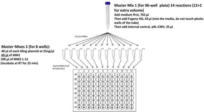
Refer to Procedures steps 28-34 for additional details.

• ▴ CRITICAL Pipet directly into the medium and avoid touching the plastic walls of the tube. Chemical residues in plastic vials can significantly decrease the biological activity of the reagent.

Add 35 μl of internal control, pRL-CMV, at 10 ng/μl.

Next, make Master Mix 2s (MM2) for 12 reactions (columns) per plate, each reaction to be distributed into 8 wells (rows) each + 2 for extra volume (see Fig. 4). Aliquot 40 μl of each test plasmid at 25 ng/μl into 12 eppendorf tubes

• ! CAUTION In order to compare activities of different tiles, plasmids containing different tiles should be transfected in the same molarity. As all our tiles are designed to have the same approximate 2Kb the same DNA concentration can be used in every transfection. However, when clones contain tiles of variable size, concentrations should be adjusted to have the same molarity in every reaction. In this case use carrier DNA (salmon sperm) to adjust the total amount of DNA being transfected.

Add 60 μl of MM1 into each eppendorf tube and incubate at RT for 25 min, then dispense 10 μl of MM2 into each well of the same column (e.g. wells A-H)

Each column will therefore have eight replicates of the same plasmid. It is recommended to add all three controls to every plate: pGFP (for transfection efficiency), pGL3-Control Vector (positive control containing SV40 enhancer), and pGL3-LRR or pGL3-LRF (negative controls; empty destination vectors containing the ccdB cassette but no enhancer). Although we transfect 8 wells with pGFP, this is only for convenience when preparing the master mixes and fewer wells (e.g. 4) are enough to monitor transfection and you may reduce the volume of the master mix for that transfection only.

Equipment Setup

Setup for luminometer (SpectraMax L) reading

1. Open the SoftMax Pro program.

2. Go to Protocols (on the toolbar) → Reporter Assays → Dual-Glo Luciferase_SpectraMax L. A new untitled document will open.

3. Scroll down that document until you see PlateA_Firely and click on Settings for that plate. A new window will open.

4. On the left panel

   1. set Integration Time to 12 sec
   2. Enable Automix
   3. Select wells to be read

5. Click OK. A table (representing a 96-well plate) will appear under PlateA_Firefly.

6. Click on the new table to set up the template. A new window will open.

7. In the top panel, under [Groups] select Firefly, then name your sample. In the bottom panel under [Layout] select the wells that correspond to that sample and click [Assign]

8. After you have entered all your samples click “OK.” The window will close and you will go back to the initial untitled document.

9. Scroll down to PlateB_Renilla and click on [Settings] for that plate and repeat steps 4-8.

10. To save the document, go to [File] on the toolbar → “Save As”

11. To connect to the luminometer, go to [SpectraMax L] under the toolbar. A new window will open.

12. Under Reader Settings (in the top, left corner of the new window)

    1. select [SpectraMax L] from the “Reader:” drop-down menu
    2. select the appropriate port from the [Connection:] drop-down menu. Note: This selection may vary depending on your connection set up. Click [OK]

Procedure

Choice of region •TIMING ∼4 h

1| Create a BED file containing SNP coordinates using the LDlink tool³⁶ (option A), SNAP (SNP Annotation and Proxy Search (option B), or directly download data from 1000 genomes project using pLink (option C).

A. LDlink (recommended)³⁶

1. Go to LDlink (http://analysistools.nci.nih.gov/LDlink/).

2. Click on [LDProxy] Tab and enter the SNP(s) rs number(s) on the left and select the desired populations (those used in the GWAS of interest) from the dropdown box (ie, “CEU”).

3. Click [Calculate] to obtain the LDProxy output. The output provides an interactive graph that plots R² of proxy SNPs and combined recombination rate against genomic coordinates. Each SNP is shown as a circle with a number inside corresponding to the RegulomeDB score for that SNP. Hover over the SNP to view more information.

4. Click [Download all proxy SNPs] at the bottom of the page to download a text (.txt) file with genomic coordinates in UCSC version hg19 (NCBI build GRCh37) format, so these can be used to create a custom .bed file to be displayed on the UCSC Genome Browser.

5. Create a BED file with your SNP coordinates. The .bed file format can be reviewed at http://genome.ucsc.edu/FAQ/FAQformat.html#format1. Use a spreadsheet program (such as Microsoft Excel) to open your .txt file from LDProxy (See examples in Supplementary Table 1, LDproxy1 sheet). In the Text Wizard, select ‘delimited’, then click ‘Next’. Under [Delimiters] check ‘Tab’ and ‘Other’. In the ‘Other’ box add a colon [:] and click ‘Next’. Under [Column data format] select ‘General’, then click ‘Finish’.

6. Select Column C and select ‘Format cells’. Under [Category] select ‘Number’ and indicate ‘0′ decimal places, then click ‘OK’. This will convert the coordinates from scientific notation to a regular number (LDProxy2 sheet). Insert a column between B and C (LDProxy3 Sheet). In the second row of the new empty column C, put in function =D2-1 (LDProxy4 sheet). Copy the function to all remaining rows until all SNPs have a start and end coordinate (LDProxy5 sheet). Choose your r² threshold (for example, start with 0.2) and delete the entries that do not meet the threshold (LDProxy6 sheet). Delete row for all columns and delete columns E-L. Move column A to column E, so that you now have chromosome number, start coordinate, end coordinate, and SNP number in four columns, in that order (LDProxy7 sheet).

B. SNAP

1. Go to SNAP (SNP Annotation and Proxy Search; http://www.broadinstitute.org/mpg/snap/index.php).

2. Click on [Proxy Search] Tab and enter the SNP(s) rs number(s).

3. Under [Search Options] choose appropriate settings. We recommend using ‘1000 Genomes Pilot 1′ as the SNP dataset, ‘500’ as the Distance limit and choose your r² threshold (start with 0.2).

4. Under [Output Options] choose download to ‘File’ and check the box to include each query SNP as a proxy for itself.

5. Under [Filter by Array] we leave all boxes unchecked. This will generate a text (.txt) file of all candidate SNPs in the locus and their genomic coordinates.

   ! CAUTION SNAP outputs coordinates in UCSC version hg18 (NCBI Build 36.1) and does not include the latest version of the 1000 Genomes Project SNPs (Phase 3).

6. Create a BED file with your SNP coordinates. Use a spreadsheet program (such as Microsoft Excel) to open your .txt file from SNAP (See examples in Supplementary Table 1, SNAP1 sheet). Insert a column between G and H (SNAP2 sheet). In the second row of the new empty column H, put in function =I2-1 (SNAP3 sheet). Copy the function to all remaining rows until all SNPs have a start and end coordinate (SNAP4 sheet). Move column B (Proxy) to column J (SNAP5 sheet). Delete the first row of every column (headings) and delete columns A-F, so that you now have chromosome number, start coordinate, end coordinate, and SNP number in four columns, in that order (SNAP6 sheet).

7. In the Human Genome Browser Gateway (http://genome.ucsc.edu/cgi-bin/hgGateway) top navigation bar go to ‘Tools’ and click on [LiftOver]. Copy A-D columns (without the headings) into LiftOver. Choose NCBI36/hg18 as [Original Assembly] and your assembly of choice (e.g. GRCh37/hg19 or GRCh38/hg38) as [New Assembly]. Hit submit and then select “View Conversions” to retrieve your converted BED file.

C. Download from 1000 genomes project (expert users)

1. If you are familiar with pLink and vcf files, directly downloading data from 1000 genomes project may provide more extensive annotation than SNAP. Download 1000 genomes genotype data for the coordinates and population of interest. The 1000 genome project provides the Data Slicer tool at http://browser.1000genomes.org/Homo_sapiens/UserData/SelectSlice?db=core. This will allow you to download a VCF file for the chromosomal region and population of interest. The file URL is already populated for chromosome 1. Edit the chromosome only.

2. Select region of interest (e.g. 9:16415021-17415021). Coordinates are in b37/hg19 assembly.

3. Select ‘No filtering’ under [VCF filters] if you wish to use all data. Select ‘By populations’ if you wish to use only specific populations. This will prompt a page where you select the populations from a scroll-down list. Click ‘Next’ and download the VCF file.

4. Use PLINK version 1.9 to run LD calculations directly on the VCF file. You can run LD calculations for a single SNP or you can run for a list of SNPs. Please see PLINK documentation for description of options and other options available. The examples below use r2 threshold of 0.2 (--ld-window-r2) and a 500kb region around the SNP (--ld-window-kb) with no limits on the number of SNPs (--ld-window 99999). The output file includes pairwise LD calculations for SNPs (SNP_A and SNP_B).

   plink --vcf genotypes –r2 --ld-snp rs3814113 --ld-window-kb 500 –ld-window 99999 –ld-window-r2 0.2 --out rs3814113_calculations

   plink --vcf genotypes –r2 --ld-snp-list snp_list.txt --ld-window-kb 500 –ld-windo w 99999 –ld-window-r2 0.2 --out list_calculations

   CRITICAL STEP: VCF option is only available for version 1.9 which is available for download at http://pngu.mgh.harvard.edu/∼purcell/plink/plink2.shtml. Previous versions require PED and MAP files. 1000 genomes Project provides the VCF to PED converter tool at http://browser.1000genomes.org/Homo_sapiens/UserData/Haploview?db=core. PED and INFO files can be downloaded from the converter tool and require slight reformatting (i.e. Chromosome column added to info file for MAP format) to use in PLINK for LD calculations.

5. Create a BED file from .LD output file. Use Excel to open and reformat the LD file. Keep CHR_B, BP_B, SNP_B columns. Insert end coordinate as BP-1.

2| Upload the BED file onto UCSD Genome Browser as follows: from the Genome Browser top navigation bar go to ‘My Data’ and select [Custom Tracks]. Choose your BED file to upload and hit Submit. Note that if you want to give your track a custom name and description, you can add a header at the top of your BED file. Example: track name=“LD SNPs” description=“LD SNPs” visibility=1 color=153,50,204. The browser window will show a map of your region of study.

3| Under [Mapping and Sequencing Tracks], toggle [BAC End Pairs] to ‘full’.

4| Choose appropriate BAC(s) covering the region of interest and click on it to obtain BAC information. Click on the BAC designation to be directed to the NCBI's CloneDB record for the BAC, click on the [Distributors] tab to choose supplier, and order BAC from supplier of choice for use in Step 12A.

CRITICAL STEP:Genomic DNA from cell lines can also be used as template to amplify tiles (see Step 12B) but using BACs increases the success rate and diminishes specificity issues.

5| Return to the browser window showing your region. Under [View], on the top menu bar, click on ‘DNA’. Verify that the region shown matches the coordinates of your region. Using the boxes under [Sequence Retrieval Options] add 2,000 extra bases to each side of the region. Example: “Add [2,000] extra bases upstream (5′) and [2,000] extra downstream (3′)”

6| Click on [get DNA]. This will generate a FASTA file with the nucleotide sequence for your region.

Primer Design •TIMING ∼4 h

7| Go to PCRTiler (http://pcrtiler.alaingervais.org:8080/PCRTiler/) and input your sequence from Step 6. For primer parameters we use Minimum primer Tm = 57; Maximum primer = 63; Amplicon range between 1800 – 2300. For tiling parameters check [Design a primer pair at each X base pairs, where X is] and enter 1800. If you are using BAC as a template (see Step 12A), check [Skip the specificity check]. This will generate a list of primer pairs to amplify the tiles.

8| Go to the Human Genome Browser Gateway (http://genome.ucsc.edu/cgi-bin/hgGateway) and under [Tools], on the top menu bar, click on ‘In silico PCR’. In the ‘Genome’ pull-down menu select ‘Human’; In the ‘Assembly’ menu select ‘Feb. 2009 (GRCh 37/hg19)’; In the ‘Target’ menu select ‘genome assembly’. For ‘Max Product Size’, ‘Min Perfect Match’, ‘Min Good Match’ retain default values. For each PCR primer pair from Step 7, copy and paste each sequence in the ‘Forward Primer’ and ‘Reverse Primer’ boxes. Click ‘submit’. Obtain the coordinates for your tiles defined by the PCR primers from the header line (it will be the first line, indicated by a ‘>’ sign) of the FASTA file:

>chr22:31000551+31001000 TAACAGATTGATGATGCATGAAATGGG CCCATGAGTGGCTCCTAAAGCAGCTGC

Add the data to an excel spreadsheet in BED file format, e.g.:

Tile 1

Chr22

31000551

31001000

9| Create a Human Genome Browser private session to keep track of your tiles. Under [My Data] on the top menu bar, click on ‘sessions’ and follow instructions to create your session.

Create a custom track and upload your BED file from Step 8 into your session in the genome browser.

10| To design primers to generate tiles by recombination add LR recombination sites (attL1 5′-CCAACTTTGTACAAAAAAGCAGGCT-3′ and attL2 5′-CCAACTTTGTACAAFAAAGCTGGGT-3) and a MluI (ACGCGT) and XhoI (CTCGAG) restriction sites to attL1 and attL2, respectively to the 5′end of the primers.

CRITICAL STEP: Alternatively, primers could be designed to generate tiles by traditional cloning. PCR primers to amplify each tile should contain the desired restriction site present in the multiple cloning site (KpnI, SacI, MluI, NheI, XhoI, BglII). For example, a forward primer would contain a KpnI site and a reverse primer would contain a BglII site. To test all tiles in both orientations, for this example PCR primers would also be generated with a BglII site in the forward primer and a KpnI site in the reverse primer. Generating clones by recombination is significantly more efficient than by traditional restriction digest cloning.

! CAUTION Some restriction enzymes are not efficient at cutting close to the end of the PCR product. We recommend consulting the New England Biolabs guide to cleavage close to the end of DNA fragments (https://www.neb.com/tools-and-resources/usage-guidelines/cleavage-close-to-the-end-of-dna-fragments) before designing primers. If you conduct traditional cloning your empty vector control should be pGL3-Promoter.

11| Order primers containing LR recombination sites and restriction digest sites. To save time you may choose to start culturing cells for cDNA isolation or order BAC clones at this stage (see Step 12).

▪ PAUSE POINT Work can re-start when BAC and primers are received.

Tile generation •TIMING ∼2 weeks

12| Obtain BAC DNA (option A) or genomic DNA (option B) to use as template to generate tiles by PCR amplification

A. BAC DNA

1. Inoculate an aliquot of the glycerol stock of E. coli containing the BAC DNA into 50-100 ml of LB containing the appropriate antibiotic for selection and incubate with shaking (at 300 rpm) overnight at 37°C.

2. Isolate BAC DNA using HiSpeed^® Plasmid Maxi kit, or Plasmid Maxi Kit following manufacturer's instructions. In our hands both kits yield similar results. CRITICAL STEP: Large Construct Kit can also be used but, in our experience yield is seldom satisfactory. ? TROUBLESHOOTING

B. Genomic DNA

1. Grow 1-2 100 mm plates of a human cell line and harvest to isolate genomic DNA. We recommend the use of normal primary or immortalized cells to avoid possible problems with genomic alterations in cancer cell lines. ! CAUTION We recommend avoiding cell lines commonly misidentified or cross-contaminated (http://iclac.org/databases/cross-contaminations/). Cell lines should be regularly checked for authenticity (for example, using Short Tandem Repeat authentication) and for Mycoplasma contamination.

2. Isolate human genomic DNA using PureLink Genomic DNA Mini Kit, following manufacturer's instructions.

13| Perform PCR to amplify tiles (see REAGENT SETUP for experimental design considerations; use 50 ng BAC DNA from Step 12Aii or amend volumes shown to allow for 100 ng if using genomic DNA from Step 12Bii.

! CAUTION Be extremely careful when manipulating primers for this experiments to avoid cross-contamination.

14| Run PCR products on 1% Agarose gel electrophoresis for size documentation and for gel purification. Recommended voltage is 4-10V/cm of distance between the electrodes). For confirmation and size documentation run 5 μl of PCR product with 1 μl of 6x Gel loading buffer. For gel purification run the remaining 20 μl (for KAPA HiFi; or 45 μl for HotStart Taq) of PCR product and 4 μl of 6x Gel loading buffer. Purify PCR products using Qiaquick gel purification kit following manufacturer's instructions.

? TROUBLESHOOTING

15| To clone each tile in both orientations, mix 7 μl of PCR product with 1 μl (150 ng) of pGL3-LRR in one eppendorf tube and, in a separate eppendorf tube mix 7 μl of PCR product with 1 μl (150 ng) of pGL3-LRF.

16| Thaw the LR Clonase enzyme mix on ice and add 2 μl to the reaction from Step 15, mix well by vortexing briefly twice and incubate 3 h to overnight 25°C.

17| Add 1 μl proteinase K to each sample and incubate at 37°C for 10 min.

Tile cloning •TIMING ∼1 week

18| Transform 50 μl of competent TOP10 E.coli using 5 μl of each LR reaction from Step 17. In our experience this reaction is successful >93%. Take this opportunity to transform, in parallel, all plasmids needed for the transfection (pGFP; pRL-CMV Renilla; pGL3-LR, and pGL3-LR-ENH) in addition to the tiling clones. For these plasmids use 1 to 5μl of DNA (typically 10-50 ng) to transform 50 μl of competent TOP10 E.coli.

19| Incubate on ice for 30 min.

20| Heat shock at 42°C for 30 sec.

21| Add 250 μl of SOC media and incubate at 37°C for 1 h with shaking.

22| Plate 20 μl onto LB/Agar Ampicillin plates and grow overnight in a 37°C incubator.

? TROUBLESHOOTING

23| Pick 1 colony and grow in 4 ml media in a 14 ml polypropylene round bottom tube overnight.

24| Isolate plasmid DNA using Qiagen mini-prep kit to confirm inserts.

25| Digest with MluI and XhoI (see REAGENT SETUP for details) for 1 hr at 37°C and run on a 1% agarose gel for verification. If size of insert is correct, make glycerol stocks of the transformants for future use. Add 500 μl of bacterial culture to 500 μl of sterile 50% glycerol (in water) in a cryotube vial and mix. Freeze the tubes at -80°C (tubes can be stored for several years).

26| Sequence clones to confirm both strands using pGL3-Seq-Rev and RVprimer3. Additional internal primers specific to each region may need to be designed to cover the entire region and verify the SNP allele.

▪ PAUSE POINT Glycerol bacterial stocks or plasmid DNA can be stored for several years at -80°C.

27| Bring all plasmid DNAs to 25 ng/μl with water to prepare for transfection. Freeze at -20°C.

▴ CRITICAL STEP All plasmids to be compared in the same batch of Luciferase assays must be prepped the same day (including controls). We have found that the same plasmid prepared in different batches (e.g. grown on separate days or stored for different lengths of time) may differ significantly in activity when transfected in parallel ³⁷.

Transfection and luciferase activity measurement •TIMING ∼1 week

28| Day 1. Plate cells. Cell to be used in the assay should be chosen with consideration for the tissue or cell type relevant for the experimental model. For example, when examining a susceptibility locus for breast cancer one would use a normal mammary gland epithelial cell line such as MCF10A (see Choice of template, tile verification, and host cell). Cells are plated at 5 × 10³/well in 40 μl of tissue culture medium a 96 well plate and incubate for 24 h. The number of cells per well is given as a guide and may need to be optimized according to cell type and transfection reagent.

29| Day 2. Set up transfection for 96 well plates (one 96 well plate) according to schema in Fig. 4. We recommend setting up one plate at a time, handling multiple plates may lead to variation in incubation times.

30| Prepare test plasmids (pGL3-LR and pGL3-LR-ENH control plasmids, pGL3 constructs containing the desired tiles) at 25ng/μl, and internal control (pRL-CMV Renilla) at 10ng/μl

31| Aliquot 40 μl of test plasmids (25ng/μl) in each eppendorf tube

32| Prepare Master mix 1 (MM1) (See reagent Setup)

33| Prepare Master mixes 2 (MM2) (See reagent Setup) by adding 60 μl of MM1 to each eppendorf tube from step 31. Mix by vortexing and incubate at RT for 25 min

34| Dispense 10 μl of MM2 into each well of the same column (e.g. wells A-H). Incubate for 24 h.

▴ CRITICAL STEP Since many tiles in different orientations and eight replicates are being analyzed it is important to have a gauge of how well the transfection worked so that reagents are not wasted on a large transfection experiment that failed. We recommend the inclusion of a GFP only transfection to monitor the general quality of transfection. In our experience, if no or very few cells are green, the transfection was inefficient and should be repeated.

? TROUBLESHOOTING

35| Day 3. Using Dual-Glo luciferase reagents measure Renilla and firefly luciferase activity 24h post transfection (see EQUIPMENT and REAGENT SETUP). For experiments with a large amount of plates, keep the time between transfection and addition of luciferase assay buffers across plates consistent. Follow manufacturer's protocol (Promega) to prepare the reagents. Using a multi-channel pipette add a volume of Dual-Glo Luciferase Reagent equal to the volume of culture medium (50μl/well)

36| Incubate at RT for 20 min to allow cell lysis

37| After completing set up for luminometer reading (EQUIPMENT SETUP section) Insert the plate with the Dual-Glo Luciferase Reagent in the luminometer.

! CAUTION Make sure to remove the plate cover before inserting the plate in the luminometer to prevent damage to the injectors!

38| Go to your protocol document and select the firefly plate to read first. Click [Read] under the toolbar. Reading of a full 96-well plate takes approximately 20 min.

39| Remove the plate, add the Dual-Glo Stop & Glo reagent, incubate for 10 min, insert plate back into the luminometer. ! CAUTION Make sure to remove the plate cover!

40| Go to your protocol document and select the Renilla plate and click [Read]. After the plate reading is finished, go to “File” → [Save] to save the readings. To export the readings go to [File] → [Export] to export your data as a txt document.

41| Obtain Firefly/Renilla luciferase ratios for each transfected well and calculate the average of the 8 wells for the empty vector (pGL3-LRR or pGL3-LRF).

42| To plot the values as fold-change over the empty vector, divide the values of the tiles by the value of the empty vector.

43| For Statistical Analysis open the GraphPad Prism 6 (or equivalent) program

44| Select “Column” under “New Table & Graph”

45| Select “Enter replicate values” under “enter/import data” from step 42, and click “Create”.

46| Copy/paste your values from step 45 in a table listing as follows: Empty vector, Enhancer, sample 1, sample 2, etc… Note: you can rename your new table by right-clicking on it. This will also change the name of the graph associated with that data.

47| Next, on the left panel click on the document under [Graphs]. This will appear as ‘Data 1” if you did not rename it. Label the X and Y axes titles by clicking on it. Note: You can edit almost anything on the graph by double clicking or right clicking on it.

48| On the graph document click on [Analyze] icon on the toolbar, a new window will open. On the left panel select ‘t tests’ under [Column Analysis]. On the right panel select just the sample you are analyzing and the empty vector. Click ‘OK’

49| In the next window select “unpaired” under “experimental design”, “Yes” under “Assume Gaussian Distribution” and “unpaired t test” under Choose test. Click “OK”. In the results page, pay attention to raw 8-10 to look for significant difference between the two compared values. The actual p value will be displayed along with the p value summary (or level of significance) and on raw 10 it will display whether it is significant or not. The statistical threshold is p value ≤ 0.05.

50| Repeat steps 26-49. Tiles that are significant in two separate experiments performed on different days are considered positive for transcription activity.

Mutagenesis to test alternative allele •TIMING ∼2 weeks

51| Design primers for QuickChange mutagenesis. We recommend Agilent link for QuickChange II which offers video tutorials (http://www.genomics.agilent.com/en/Site-Directed-Mutagenesis/QuikChange-II/?cid=AG-PT-175&tabId=AG-PR-1161) and free access to a primer design program. For tiles with multiple SNPs, mutagenesis can be done for each individual SNP separately to tease out individual contributions.

52| Perform QuickChange mutagenesis using QuikChange II XL Site-Directed Mutagenesis Kit (Agilent) according to manufacturer's instruction.

53| Return to Step 18 and transform 50 μl of competent TOP10 E.coli using 5 μl of each QuickChange reaction and continue through step 49 comparing tiles with the major allele to tiles with the minor allele (not with the empty vector as in initial experiments). If they display significant differences in activity they will be considered to have allele-specific activity.

Troubleshooting

Troubleshooting advice can be found in Table 1.

Anticipated Results

At the end of the protocol we anticipate that the investigator will have generated tiles representing the genomic region of interest and will have identified genomic tiles that contain regulatory elements activated by factors present in the transfected cell (Fig. 5A). These tiles can then be reduced to narrow down the region and they can be mutagenized to test whether different alleles of SNPs contained in the tile have specific effects. The results provide an empirical map of regulatory activity operating in the locus for the cell lines tested. While 95% of the human genome lies within 8 kb of a DNA-protein interaction site¹⁵ not all experiments will necessarily detect a regulatory region with activity significantly different than the empty vector control. However, tiles can only be discarded if they fail in both orientations in at least two independent experiments. The positive control plasmid (pGL3-control) contains strong SV40 enhancer and promoter sequences and is expected to show luciferase activities 5-40 fold depending on the cell line. An experiment should be discarded if the positive control, in a specific a cell line that usually yields 20-fold activities over the negative control, results in much lower activities. Compare Figs. 5A and B and note that tiles that are significant in A are not identified in B. Tiles that show significant activities can then be mutagenized to change the SNP alleles under study to determine whether they are functionally significant. The results provide an empirical map of regulatory activity operating in the locus for the cell lines tested.

Figure 5. Typical anticipated results.

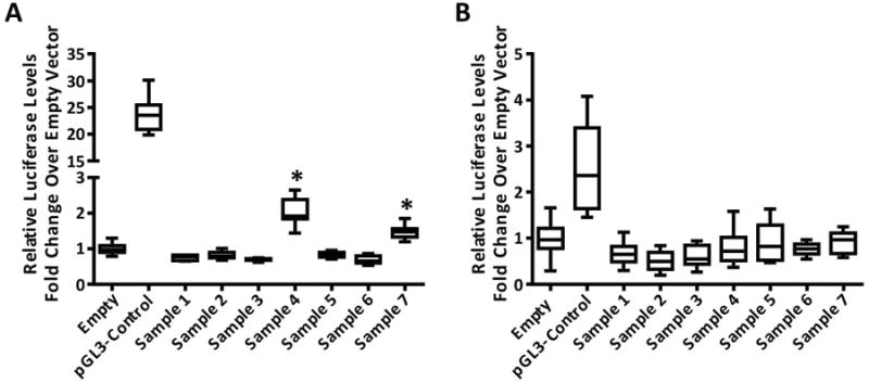
Two separate experiments testing the same tile in the same cell line. Results from an immortalized ovarian cell lines transfected with Fugene HD according to the protocol described here and plotted as box-and-whisker plots. Boxes represent the interquartile range (IQR, difference between upper and lower quartiles). The median is indicated by the horizontal line within the box. Lower and upper bars represent Q1 (first quartile; 25% percentile) – 1.5× IQR, and Q3 (third quartile; 75% percentile) – 1.5× IQR, respectively. Experiment in A the positive control (containing an SV40 enhancer and promoter) displayed 20-25× the activity of the negative (empty vector) control used as the reference. Two tiles are found to be significant (*, p ≤ 0.05; Samples 4 and 7). However, in B no tile is significantly higher than the negative control but the relative low activity of the positive control (2-3× the activity of the negative control) indicates a suboptimal transfection that should be discarded and the experiment repeated before eliminating tiles from analysis.

Timing

Steps 1-11: WEEK 1. 1-2 days of hands-on effort

Steps 1-6: 4 hours. For those with no experience with the use of the UCSC Human Genome Browser it is highly recommended to follow the tutorial materials available (http://www.nature.com/scitable/ebooks/guide-to-the-ucsc-genome-browser-16569863). In this case the user should estimate an additional 2-3 hours to these steps.

Steps 7-11: 4 hours. Delivery for oligonucleotide primers may take from a few days to more than a week depending on location.

Steps 12-26: WEEK 2-4

Step 12A. 2-day procedure with ∼4 hours of hands-on effort

Step 12B. 5-day procedure with ∼4 hours of hands-on effort. Both steps can be performed while you wait for primer delivery.

Steps 13-26. Depending on the number of PCR tiles to be generated and the efficiency estimate between 1-2 weeks to obtain all desired clones. Confirmation by Sanger sequencing may depend on vendor or core facility but many offer a 2-day turnaround.

Steps 27-50. WEEK 5-6

It is estimated six full days of hands-on effort for transfections, luciferase measurements and data analysis (accounting for a minimal number of biological replicates – independent transfections). Depending on the number of tiles these steps can take one or two weeks. Having parallel cultures for transfection can reduce the time to complete experiments with biological replicates, but it is recommended to allow sufficient time for completion of the previous step before proceeding.

Steps 51-53. WEEK 7-8

Similar to Steps 10-26. To save time these steps can be performed concurrently with Steps 10-26, in particular if it is a small number of clones.

Supplementary Material

Supplementary Table 1

Supplementary table 1. Steps to generate a BED file containing SNP coordinates from LDlink or SNAP Proxy. Contains step by step examples of data generated from LDlink or SNA Proxy and being formatted for uploading onto the UCSC Human Genome Browser.

References

- 1.Manolio TA. Genomewide association studies and assessment of the risk of disease. The New England journal of medicine. 2010;363:166–176. doi: 10.1056/NEJMra0905980. [DOI] [PubMed] [Google Scholar]
- 2.Lewis CM, Knight J. Introduction to genetic association studies. Cold Spring Harbor protocols. 2012;2012:297–306. doi: 10.1101/pdb.top068163. [DOI] [PubMed] [Google Scholar]
- 3.Freedman ML, et al. Principles for the post-GWAS functional characterization of cancer risk loci. Nature genetics. 2011;43:513–518. doi: 10.1038/ng.840. [DOI] [PMC free article] [PubMed] [Google Scholar]
- 4.Edwards SL, Beesley J, French JD, Dunning AM. Beyond GWASs: illuminating the dark road from association to function. American journal of human genetics. 2013;93:779–797. doi: 10.1016/j.ajhg.2013.10.012. [DOI] [PMC free article] [PubMed] [Google Scholar]
- 5.Monteiro AN, Freedman ML. Lessons from postgenome-wide association studies: functional analysis of cancer predisposition loci. Journal of internal medicine. 2013;274:414–424. doi: 10.1111/joim.12085. [DOI] [PMC free article] [PubMed] [Google Scholar]
- 6.Tang W, et al. Mapping of the UGT1A locus identifies an uncommon coding variant that affects mRNA expression and protects from bladder cancer. Human molecular genetics. 2012;21:1918–1930. doi: 10.1093/hmg/ddr619. [DOI] [PMC free article] [PubMed] [Google Scholar]
- 7.Maurano MT, et al. Systematic localization of common disease-associated variation in regulatory DNA. Science. 2012;337:1190–1195. doi: 10.1126/science.1222794. [DOI] [PMC free article] [PubMed] [Google Scholar]
- 8.Sakoda LC, Jorgenson E, Witte JS. Turning of COGS moves forward findings for hormonally mediated cancers. Nature genetics. 2013;45:345–348. doi: 10.1038/ng.2587. [DOI] [PubMed] [Google Scholar]
- 9.Chung CC, Magalhaes WC, Gonzalez-Bosquet J, Chanock SJ. Genome-wide association studies in cancer--current and future directions. Carcinogenesis. 2010;31:111–120. doi: 10.1093/carcin/bgp273. [DOI] [PMC free article] [PubMed] [Google Scholar]
- 10.Carey M, Smale ST. Transcriptional regulation in eukaryotes: Concepts, strategies and techniques. Cold Spring Harbor Laboratory Press; 1999. [Google Scholar]
- 11.Pharoah PD, et al. GWAS meta-analysis and replication identifies three new susceptibility loci for ovarian cancer. Nature genetics. 2013;45:362–370. doi: 10.1038/ng.2564. [DOI] [PMC free article] [PubMed] [Google Scholar]
- 12.Baskin R, et al. Functional analysis of the 11q23.3 glioma susceptibility locus implicates PHLDB1 and DDX6 in glioma susceptibility. Scientific Reports. 2015 doi: 10.1038/srep17367. in press. [DOI] [PMC free article] [PubMed] [Google Scholar]
- 13.Neph S, et al. An expansive human regulatory lexicon encoded in transcription factor footprints. Nature. 2012;489:83–90. doi: 10.1038/nature11212. [DOI] [PMC free article] [PubMed] [Google Scholar]
- 14.Thurman RE, et al. The accessible chromatin landscape of the human genome. Nature. 2012;489:75–82. doi: 10.1038/nature11232. [DOI] [PMC free article] [PubMed] [Google Scholar]
- 15.Dunham I, et al. An integrated encyclopedia of DNA elements in the human genome. Nature. 2012;489:57–74. doi: 10.1038/nature11247. [DOI] [PMC free article] [PubMed] [Google Scholar]
- 16.Sanyal A, Lajoie BR, Jain G, Dekker J. The long-range interaction landscape of gene promoters. Nature. 2012;489:109–113. doi: 10.1038/nature11279. [DOI] [PMC free article] [PubMed] [Google Scholar]
- 17.Djebali S, et al. Landscape of transcription in human cells. Nature. 2012;489:101–108. doi: 10.1038/nature11233. [DOI] [PMC free article] [PubMed] [Google Scholar]
- 18.Gerstein MB, et al. Architecture of the human regulatory network derived from ENCODE data. Nature. 2012;489:91–100. doi: 10.1038/nature11245. [DOI] [PMC free article] [PubMed] [Google Scholar]
- 19.Andersson R, et al. An atlas of active enhancers across human cell types and tissues. Nature. 2014;507:455–461. doi: 10.1038/nature12787. [DOI] [PMC free article] [PubMed] [Google Scholar]
- 20.FANTOM Consortium et al. A promoter-level mammalian expression atlas. Nature. 2014;507:462–470. doi: 10.1038/nature13182. [DOI] [PMC free article] [PubMed] [Google Scholar]
- 21.Stergachis AB, et al. Exonic transcription factor binding directs codon choice and affects protein evolution. Science. 2013;342:1367–1372. doi: 10.1126/science.1243490. [DOI] [PMC free article] [PubMed] [Google Scholar]
- 22.Mansour MR, et al. Oncogene regulation. An oncogenic super-enhancer formed through somatic mutation of a noncoding intergenic element. Science. 2014;346:1373–1377. doi: 10.1126/science.1259037. [DOI] [PMC free article] [PubMed] [Google Scholar]
- 23.Melnikov A, et al. Systematic dissection and optimization of inducible enhancers in human cells using a massively parallel reporter assay. Nature biotechnology. 2012;30:271–277. doi: 10.1038/nbt.2137. [DOI] [PMC free article] [PubMed] [Google Scholar]
- 24.Arnold CD, et al. Genome-wide quantitative enhancer activity maps identified by STARR-seq. Science. 2013;339:1074–1077. doi: 10.1126/science.1232542. [DOI] [PubMed] [Google Scholar]
- 25.Plank JL, Dean A. Enhancer function: mechanistic and genome-wide insights come together. Molecular cell. 2014;55:5–14. doi: 10.1016/j.molcel.2014.06.015. [DOI] [PMC free article] [PubMed] [Google Scholar]
- 26.van Arensbergen J, van Steensel B, Bussemaker HJ. In search of the determinants of enhancer-promoter interaction specificity. Trends in cell biology. 2014;24:695–702. doi: 10.1016/j.tcb.2014.07.004. [DOI] [PMC free article] [PubMed] [Google Scholar]
- 27.Carlson CS, et al. Selecting a maximally informative set of single-nucleotide polymorphisms for association analyses using linkage disequilibrium. American journal of human genetics. 2004;74:106–120. doi: 10.1086/381000. [DOI] [PMC free article] [PubMed] [Google Scholar]
- 28.Hazelett DJ, et al. Comprehensive functional annotation of 77 prostate cancer risk loci. PLoS genetics. 2014;10:e1004102. doi: 10.1371/journal.pgen.1004102. [DOI] [PMC free article] [PubMed] [Google Scholar]
- 29.French JD, et al. Functional variants at the 11q13 risk locus for breast cancer regulate cyclin D1 expression through long-range enhancers. American journal of human genetics. 2013;92:489–503. doi: 10.1016/j.ajhg.2013.01.002. [DOI] [PMC free article] [PubMed] [Google Scholar]
- 30.Boyle AP, et al. Annotation of functional variation in personal genomes using RegulomeDB. Genome research. 2012;22:1790–1797. doi: 10.1101/gr.137323.112. [DOI] [PMC free article] [PubMed] [Google Scholar]
- 31.Coetzee SG, Rhie SK, Berman BP, Coetzee GA, Noushmehr H. FunciSNP: an R/bioconductor tool integrating functional non-coding data sets with genetic association studies to identify candidate regulatory SNPs. Nucleic acids research. 2012;40:e139. doi: 10.1093/nar/gks542. [DOI] [PMC free article] [PubMed] [Google Scholar]
- 32.Blackwood EM, Kadonaga JT. Going the distance: a current view of enhancer action. Science. 1998;281:60–63. doi: 10.1126/science.281.5373.60. [DOI] [PubMed] [Google Scholar]
- 33.Birney E, et al. Identification and analysis of functional elements in 1% of the human genome by the ENCODE pilot project. Nature. 2007;447:799–816. doi: 10.1038/nature05874. [DOI] [PMC free article] [PubMed] [Google Scholar]
- 34.Khoury G, Gruss P. Enhancer elements. Cell. 1983;33:313–314. doi: 10.1016/0092-8674(83)90410-5. [DOI] [PubMed] [Google Scholar]
- 35.Braman J, Papworth C, Greener A. Site-directed mutagenesis using double-stranded plasmid DNA templates. Methods in molecular biology. 1996;57:31–44. doi: 10.1385/0-89603-332-5:31. [DOI] [PubMed] [Google Scholar]
- 36.Machiela MJ, Chanock SJ. LDlink: a web-based application for exploring population-specific haplotype structure and linking correlated alleles of possible functional variants. Bioinformatics. 2015 doi: 10.1093/bioinformatics/btv402. [DOI] [PMC free article] [PubMed] [Google Scholar]
- 37.Millot GA, et al. A guide for functional analysis of BRCA1 variants of uncertain significance. Human mutation. 2012;33:1526–1537. doi: 10.1002/humu.22150. [DOI] [PMC free article] [PubMed] [Google Scholar]
Associated Data
This section collects any data citations, data availability statements, or supplementary materials included in this article.
Supplementary Materials