Finite Element Modelling of the Femur Bone of a Subject Suffering from Motor Neuron Lesion Subjected to Electrical Stimulation

Abstract

Bone loss and a decrease in bone mineral density is frequently seen in patients with motor neuron lesion due to lack of mechanical stimulation. This causes weakening of the bones and a greater risk of fracture. By using functional electrical stimulation it is possible to activate muscles in the body to produce the necessary muscle force to stimulate muscle growth and potentially decrease the rate of bone loss. A longitudinal study was carried out on a single patient undergoing electrical stimulation over a 6 year period. The patient underwent a CT scan each year and a full three dimensional finite element model for each year was created using Mimics (Materialise) and Abaqus (Simulia) to calculate the risk of fracture under physiologically relevant loading conditions. Using empirical formulas connecting the bone mineral density to the stiffness and ultimate tensile stress of the bone, each element was assigned a unique material property, based on its density. The risk of fracture was estimated by calculating the ratio between the predicted stress and the ultimate tensile stress, should it exceed unity, failure was assumed. The results showed that the number of elements that were predicted to be at risk of failure varied between years.

Patients with motor neuron lesion are subjected to a decrease in bone strength in the paralysed limbs. The bones in healthy subjects are constantly under remodelling due to the loading applied either through contact forces or muscle forces. With the loss of muscle control, the muscles start to deteriorate and the bones in the affected limb do not receive enough stimulus to re-model, thus resulting in a loss of bone mineral density.¹ It has been reported that the bone mineral density (BMD) in the patella and in the tibia epiphysis for spinal cord injured patients is between 52-63% of the values for able bodied persons.² This makes the bones more susceptible to fracture. It has been shown that the bone mineral density deteriorates rapidly during the first 3-8 years post injury but at a slower rate after that.^3,4 Therefore it is important to start rehabilitation as soon as possible post injury. A new method has been developed for patients to stimulate degenerated muscles using functional electrical stimulation (FES) and to provide enough stimulus to the muscles to increase the muscle tissue and the bone mineral density for lower motor neuron lesion patients.⁵ This method has demonstrated positive effects on the patella bone where the bone mineral density increased with muscle stimulation as well as on the femur.^6,7. The finite element (FE) method is a powerful tool to evaluate the stress field in bones and numerically evaluate the fracture risk under a given loading. Using a CT imaging technique it is possible to obtain a good estimation of the material distribution within the bone, resulting in a more physiologically relevant model on a subject specific basis. However less is known about the in vivo joint contact forces and muscle forces acting on the bone. Much focus is currently on creating a fully subject specific model, based on geometry, material distribution and loading conditions.⁸ The geometry of the femur and well defined external loading conditions during activities of daily living such as gait, stance, ascension and descension in stairs etc, makes the femur popular for creating subject specific musculoskeletal models and finite element models. A few studies have looked at the fracture risk of the femur under loading and compared to series of cadaveric testing.^9,10 In the current study, finite element models of the femur were created from CT scans taken from a single paralysed young male subject over a period of 6 years. During the course of the 6 years, the subject received electrical stimulation treatment in order to try to increase muscle volume and bone mineral density in the femur.¹¹ The first stimulus treatment started 5 years post injury. Finite element analysis was carried out in order to asses the risk associated to load the femur of that particular subject. This type of risk analysis is important in order to try to estimate whether or when it would be safe to let the subject support his own weight under external muscle stimulation.

Materials and Methods

Geometric construction

CT scans were taken of the whole femur, where the in plane resolution was 0.710x0.710mm and slice thickness of 0.625 mm. The scans were obtained from a single subject between the years 2003 and 2008. Ethical permission was obtained for the study and the subject gave an informed consent for participating. The CT scans were imported into Mimics from Materialise where semi-automatic edge detection was carried out. Three-dimensional object was created of each bone and meshed using surface elements. The meshing was carried out using Magics, an automated meshing module within Mimics (Materialise). The surface elements were triangular elements, S3R. The element size was set as a maximum side length of 0.7mm and it was assumed that the aspect ratio did not go below 0.4. The surface elements were imported into Abaqus (v.6.7-1, Simulia) where 3 dimensional elements were created from the surface mesh. The tetrahedral elements were C3D10 type quadratic elements. This resulted in total number of elements over the whole femur ranging from 1,469,464 to 1,510,727 elements (average: 1,493,319). The volume of each element would be representative of the volume of each voxel from the CT scan. This high number of elements was essential in order to get a representative material distribution over the femur, explained in more detail in the following chapter.

Material assignment

The three dimensional mesh was exported from Abaqus and imported again into Mimics where the element stiffness was assigned using the Hounsfield values from the CT scans. It has been reported that discrepancy in accuracy can lie in how the Young’s modulus of each element is space between calculated and¹² missing. In general, material assignment for voxels within CT scans is based on averaging the Hounsfield units of each pixel inside each element. This method could give poor results should the element size be larger than the voxel. Therefore it was attempted to have the element size smaller or similarly sized as the voxels in order to minimize errors.

Previously published papers have addressed the relationship between the Hounsfield values and the density.¹³ It was assumed that the density was related to the Hounsfield units, using the expression obtained from Rho et al.¹⁴

The material properties were applied on the FE mesh, using the Mimics software where an average Young’s modulus was calculated from the CT dataset. Experimental data have shown that a power law exists between the Young’s modulus and the apparent density. In a finite element study of the femur carried out by Schileo et al.,⁹ three different density-stiffness expressions were applied to a finite element model of the femur and strain results were compared to experimental values. It was found that the material expression that best agreed with the experimental values was:

which was presented by Morgan et al, based on femoral neck specimens.¹⁵ The Poisson’s ratio was assumed 0.3 for the whole bone.¹⁶ With this procedure it was possible to estimate the material distribution in the bone.

Similar expressions have tried to connect together the yield strength of bone with the apparent density or the Young’s modulus. Fyhrie et al,¹⁷ published experimental data, connecting the Young’s modulus to the yield strength using a linear relation and Bessho et al connected the yield strength to the ash density through the following expression.¹⁸

The connection between the apparent density, ρ_app, and the ash density, ρash is given by the following from Yuehuei et al.¹⁹

With these expressions, it was possible to identify all the material characteristics from the CT scans. The material spectrum was divided into 10 intervals ranging from the lowest bone mineral density region (Material number 1) representing the cancellous bone to the highest bone mineral density region (Material number 10) representing the cortical bone.

Loading conditions

Loading conditions were applied according to the findings of Bergmann et al. who measured hip contact forces during various activities.²⁰ The hip contact forces were measured and presented as three dimensional forces acting on the head of the femur. In the current study, the loading scenario modelled was that of standing up. Bergmann et al. published that the maximum hip forces were as followed:²¹

• Fx=46% BW

• Fy=25% BW

• Fz=208%BW

with the forces in the following coordinate system: +ve Fx directed laterally, +ve Fy directed anteriorly and +ve Fz is directed distally. This loading scenario might represent forces which the subject is not capable of producing and the stresses calculated in the bone could indicate a high risk of failure. The subject weighed 786 N. Another set of loading conditions were applied which modelled free standing. The following force components were used in the same coordinate system

• Fx=15%BW

• Fy=3%BW

• Fz=64%BW

A set of node-points were defined at the head of the femur in order to define the placement of the loading. More than 100 node-points were manually selected from the head of the femur in order to distribute the loading in a more physiological manner, simulating the contact interaction from the acetabulum. One single force applied on one single node would generate unphysiological stress values at the point of application. The distal end of the femur was held rigid and no translation or rotation allowed for the external node-points ranging from the distal end of the femur to the femoral condyles.

Results

The simulations were run on a dual core 3GHz CPU, running Abaqus version 6.6-1 on windows 64 bit platform using 8Gb of RAM. The analysis was modelled as steady state (using the standard solver) and took 7 hours of CPU time for each bone.

Material distribution

Figure 1 shows the material distribution in the bone over the course of the 6 years, expressed as percentage of elements within each material region.. From the figure, two regions of interest can be seen, one high peak towards the low density region and another peak towards the high density region. From the material distribution it can be seen how the number of elements in the low density region changes between years. In 2005 there is the lowest count of low density material and the highest count of high density material

Figure 1.

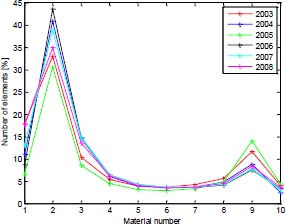
Material distribution in the bone over the 5 years.

Yield Strength and Young’s modulus values.

The expressions in section 2.2 were used to link the density to the Hounsfield units and the Young’s modulus to the density. For each of the stiffness regions the corresponding yield stress was calculated.

The von Mises stress values for each of those 10 regions were compared to the calculated yield stress and the number of elements exceeding the yield stress. Table 1 shows the Young’s modulus values for the models. By using the power law expressions between the ash density and the yield strength, the yield strength value for each of the region was calculated. The stress values were exported into Matlab where the following was extracted

Table 1.

Stiffness distribution between the bones and stiffness values

	2003	2004	2005	2006	2007	2008
	E [GPa]	E [GPa]	E [GPa]	E [GPa]	E [GPa]	E [GPa]
Region 1	0.05	0.04	0.14	0.07	0.08	0.1
Region 2	1.00	0.93	1.01	0.92	0.99	1.0
Region 3	2.54	2.36	2.30	2.57	2.40	2.49
Region 4	4.47	4.15	3.89	4.71	4.18	4.28
Region 5	6.73	6.26	5.73	7.23	6.25	6.37
Region 6	9.28	8.63	7.79	10.09	8.57	8.71
Region 7	12.08	11.23	10.05	13.24	11.13	11.29
Region 8	15.11	14.06	12.49	16.66	13.89	14.08
Region 9	18.36	17.08	15.10	20.32	16.85	17.06
Region 10	21.81	20.29	17.87	24.23	19.99	20.22

• Number of elements exceeding the yield strength of each region

• The highest value of the stresses compared to the yield strength of each region

The average fracture risk over the whole bone was calculated and compared between years. The results can be seen in Table 3.

Table 3.

Percent of elements above the yield strength and the risk factor associated

	2003	2004	2005	2006	2007	2008
% of elements above yield	3.2	5.1	1.5	4.9	12.2	8.8
Risk factor	2.1	2.5	1.6	2.3	3.4	2.6

From Table 3 it can be seen that the overall trend of elements exceeding the yield threshold is increasing with year although in 2005, the bone showed improved response to the loading and the risk of fracture decreased. The highest risk factor occurred in 2007. From all the models, the greatest proportion of elements exceeding the fracture threshold were low bone density elements, indicating that the greatest risk of fracture occurring in the cancellous bone.

3.2 Stress distribution

Von Mises stresses were plotted to represent the stresses in the femur. A stress plot of all the femurs from 2003 to 2008 can be seen in figure 2. The elements coloured in red, exceed 20 MPa. From the image it can be seen how the stress distribution changes between years under the same loading which modelled a subject standing up. From the figure it can be seen how years 2003 and 2005 stand out in the sense that higher stresses can be seen in the femoral stem than for years 2004 and 2006-2008, which is due to the increased amount of higher density bone which is able to withstand higher stresses

Figure 2.

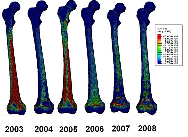
von Mises stress plots of the femur bones between 2003 and 2008 for standing up motion

Stresses around the condyles are not physiologically representable since the boundary conditions were applied there, not allowing the exterior node points to translate or rotate.

A figure of the slice through of the bones was created (Figure 3) and from that it can be seen how the stresses behave inside the bone. From the figure it can be seen how higher stresses are seen in the posterior and anterior side of the femur for years 2006, 2007 and 2008. These stresses are directly linked to the bending behaviour of the bone under the loading where the anterior is in tension and the posterior is in compression. Stress plots were also created of the loading conditions when the subject merely supports its own body weight. The stress contour plots can be seen in Figure 4.

Figure 3.

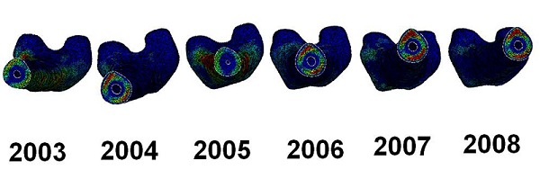
Slice through of the femur bones.

Figure 4.

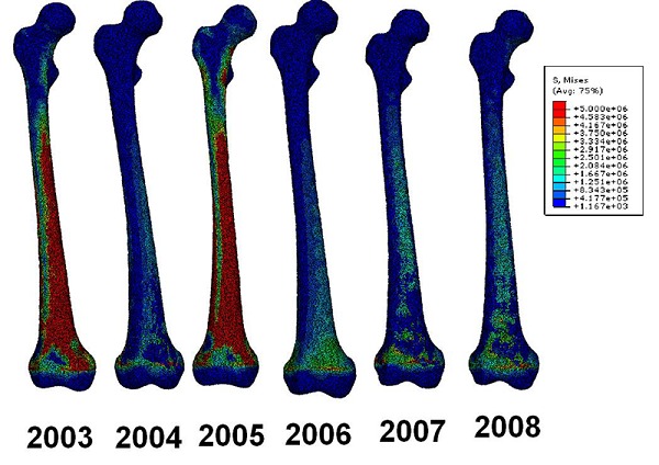
Stress contour plots for subject supporting its own body weight.

Elements coloured red in Figure 4 show stresses at or around 5 MPa. Failure risk analysis showed that all the elements were below the yield strength and little risk should be for bone failure.

Discussion

During the creation of the model, manual adjustment was involved during the edge detection process which could have resulted in geometrical errors, however care was taken keep the geometric integrity from the CT scans. The mesh was similarly sized as the voxels so that errors from interpolation between Hounsfield units should have been at minimum. The material distribution played a crucial role in identifying the stress distribution within the bone and analysing the risk fracture. An increase in the number of high density material was seen in the bone in 2005, but in the years 2006-2008, the bone showed decrease in the high density material, which is represented in the increased risk of fracture.

The patient was 20 year old at the time of injury and the stimulation treatment started 5 years post injury. It has been demonstrated how the bone density in the lower limbs decreases with time in spinal cord injury patients.^3,4 The amount of bone loss varies between individuals where the bone quality pre-injury is one of the determining factor. The patient in the presented study was given functional electrical stimulation on the thigh muscles 5 year post-injury. The treatment was divided into high/medium/low stimulus, depending on the intensity of the electric signal applied to the Rectus Femoris muscle. Table 2 shows the treatment schedule for the patient. From the table it can be seen that the intensity of the treatment varied between years and in 2004 there was little or no treatment due to diseases and burn sores. A technical fault was also reported with the stimulator toward the end of 2004. In the beginning of 2005 the subject underwent a rigorous treatment which potentially could explain the increase in the higher bone density material.

Table 2.

Treatment procedure over 5 years. Hsr=High stimulation, Msr=Medium stimulation, Lsr=Low stimulation, Ns=No stimulation, CT=time of CT scan

	2004						2005						2006						2007						2008
Time	1	2	3	4	5	6	1	2	3	4	5	6	1	2	3	4	5	6	1	2	3	4	5	6	1	2	3	4	5	6
Hsr							X	X					X	X									X					X	X	X
Msr	X	X							X		X	X					X		X	X	X	X		X	X	X	X
Lsr			X							X					X	X		X
Ns			X	X	X						X		X
CT						X			X			X					X		X							X

Analysis of the fractured elements showed that the elements most likely to exceed the failure threshold were the low density elements that were located towards the epiphyses. The greatest number of elements exceeding the yield strength were elements in material regions 1 and 2, but for the higher density bone, little or no damage could be seen.

The reported analysis does not incorporate any muscle function and solely investigates the bone behaviour under a simulated tri-axial loading test. The size of the rectus femoris muscle grew however in volume over the years of stimulation and more research is required to investigate the interaction between the intensity of FES rehabilitation and bone stimulus. The information gathered from such an analysis could provide important information about the overall bone quality of patients undergoing electrical stimulation therapies, but further research is needed to determine the effects of the electrical stimulation within microscopic regions of the bone.

There are many limitations to a study like the one presented. From the modelling aspect, the greatest limitation is in terms of how the boundary conditions are applied as creating a musculoskeletal model of an SCI patient is difficult. The load cases applied to the model represent a theoretical scenario. A more accurate method would be to create a dynamical model simulating for instance a fall from a wheelchair. In terms of clinical aspect, there are limitations in how the electrical stimulation was applied and whether patients comply fully with the daily stimulation regime. Only a single subject was selected for the finite element study, but future studies should look at a larger cohort of patients.

In conclusion, the finite element model of a single patient created annually over a 6 year period show that. the mechanical response of the load for two load cases, standing up and free standing can be calculated revealing greater risk of fracture for standing up than for free standing. The risk of fracture varied between years and it was shown that low density elements representing the cancellous bone were more prone to exceeding the fracture threshold rather than high density elements.

References

- 1.Helgason Th, Gargiulo P, Jóhannesdóttir F, et al. Monitoring muscle growth and tissue changes induced by electrical stimulation of denervated degenerated muscles with CT and stereolithographic 3D modelling. Artif Organs 2005; 29:440–3. [DOI] [PubMed] [Google Scholar]
- 2.Rittweger J, Gerrits K, Altenburg T, et al. Bone adaptation to altered loading after spinal cord injury: A study of bone and muscle strength, J Musculoskelet Neuronal Interact 2006;6: 269-76. [PubMed] [Google Scholar]
- 3.Coupaud S, McLean AN, Allan DB. Role of peripheral quantitative computed tomography in identifying disuse osteoporosis in paraplegia, Skeletal radiol 2009;38:989-95. [DOI] [PubMed] [Google Scholar]
- 4.Eser P, Frotzler A, Zehnder Y, et al. Relationship between the duration of paralysis and bone structure: a pQCT study of spinal cord injured individuals. Bone 2004;34:869-80. [DOI] [PubMed] [Google Scholar]
- 5.Gargiulo P, Vatnsdal B, Ingvarsson P, et al. Restoration of muscle volume and shape induced by electrical stimulation of denervated, degenerated muscles: qualitative and quantitative measurement of changes in Rectus Femoris using computer tomography and image segmentation. Artif Organs 2008;32:609–13. [DOI] [PubMed] [Google Scholar]
- 6.Gargiulo P, Helgason Th, Reynisson PJ, et al. Monitoring of muscle and bone recovery in spinal cord injury patients treated with electrical stimulation using three dimensional imaging and segmentation techniques: Methodological assessment. Artif Organs 2011;35:275-81. [DOI] [PubMed] [Google Scholar]
- 7.Frotzler A, Coupaud S, Perret C, et al. High-volume FES-cycling partially reverses bone loss in people with chronic spinal cord injury. Bone 2008;43:169-76. [DOI] [PubMed] [Google Scholar]
- 8.Viceconti M, Davinelli M, Taddei F, Cappello A. Automatic generation of accurate subject-specific bone finite element models to be used in clinical studies. J Biomech 2004;37:1597–1605. [DOI] [PubMed] [Google Scholar]
- 9.Schileo E, Taddei F, Malandrino A, et al. Subject-specific finite element models can accurately predict strain levels in long bones. J Biomech 2007;40: 2982–9. [DOI] [PubMed] [Google Scholar]
- 10.Schileo E, Taddei F, Cristofolini L, Viceconti M. Subject-specific finite element models implementing a maximum principal strain criterion are able to estimate failure risk and fracture location on human femurs tested in vitro. J Biomech 2008;41:356–367. [DOI] [PubMed] [Google Scholar]
- 11.Helgason Th, Gargiulo P, Ingvarsson P, Yngvason S. Using mimics to monitor changes in bone mineral density of femur during electrical stimulation therapy of denervated degenerated Thigh Muscles. Mimics Innovation awards 2007; www.materialise.com [Google Scholar]
- 12.Taddei F, Schileo E, Helgason B, et al. The material mapping strategy influences the accuracy of CT-based finite element models of bones: An evaluation against experimental measurements. Med Eng Phys 2007;29:973–9. [DOI] [PubMed] [Google Scholar]
- 13.Ciarelli MJ, Goldstein SA, Kuhn JL, et al. Evaluation of orthogonal mechanical properties and density of human trabecular bone from the major metaphyseal regions with materials testing and computed tomography. J Orthop Res 1991;9:674-82. [DOI] [PubMed] [Google Scholar]
- 14.Rho JY, Hobatho MC, Ashman RB. Relations of mechanical properties to density and CT numbers in human bone. Med Eng Phys 1995;17:347-55. [DOI] [PubMed] [Google Scholar]
- 15.Morgan EF, Bayraktar HH, Keaveny TM. Trabecular bone modulus-density relationships depend on anatomic site. J Biomech 2003;36:897–904. [DOI] [PubMed] [Google Scholar]
- 16.Wirtz DC, Schiffers N, Pandorf T, et al. Critical evaluation of known bone material properties to realize anisotropic FE-simulation of the proximal femur. J Biomech 2000;33:1325–30. [DOI] [PubMed] [Google Scholar]
- 17.Fyhrie DP, Vashishth D. Bone stiffness predicts strength similarly for human vertebral cancellous bone in compression and for cortical bone in tension. Bone 2000;26:169–73. [DOI] [PubMed] [Google Scholar]
- 18.Bessho M, Ohnishi I, Matsuyama J, et al. Prediction of strength and strain of the proximal femur by a CT-based finite element method. J Biomech 2007; 40:1745–53. [DOI] [PubMed] [Google Scholar]
- 19.Yuehuei HA, Barfield WR, Ivars K. Mechanical testing of bone and the bone-implant interface, CRC Press, Chapter: Methods of Evaluation for Bone Dimensions, Densities, Contents, Morphology and Structure. 2000;1103-19. [Google Scholar]
- 20.Bergmann G, Graichen F, Rohlmann A. Hip joint loading during walking and running, measured in two patients. J Biomech 1993;26:969-90. [DOI] [PubMed] [Google Scholar]
- 21.Bergmann G, Deuretzbacher G, Heller M, et al. Hip contact forces and gait patterns from routine activities. J Biomech 2001;34:859–71. [DOI] [PubMed] [Google Scholar]