Linear correlation between the number of olfactory sensory neurons expressing a given mouse odorant receptor gene and the total volume of the corresponding glomeruli in the olfactory bulb

ABSTRACT

Chemosensory specificity in the main olfactory system of the mouse relies on the expression of ∼1,100 odorant receptor (OR) genes across millions of olfactory sensory neurons (OSNs) in the main olfactory epithelium (MOE), and on the coalescence of OSN axons into ∼3,600 glomeruli in the olfactory bulb. A traditional approach for visualizing OSNs and their axons consists of tagging an OR gene genetically with an axonal marker that is cotranslated with the OR by virtue of an internal ribosome entry site (IRES). Here we report full cell counts for 15 gene‐targeted strains of the OR‐IRES‐marker design coexpressing a fluorescent protein. These strains represent 11 targeted OR genes, a 1% sample of the OR gene repertoire. We took an empirical, “count every cell” strategy: we counted all fluorescent cell profiles with a nuclear profile within the cytoplasm, on all serial coronal sections under a confocal microscope, a total of 685,673 cells in 56 mice at postnatal day 21. We then applied a strain‐specific Abercrombie correction to these OSN counts in order to obtain a closer approximation of the true OSN numbers. We found a 17‐fold range in the average (corrected) OSN number across these 11 OR genes. In the same series of coronal sections, we then determined the total volume of the glomeruli (TGV) formed by coalescence of the fluorescent axons. We found a strong linear correlation between OSN number and TGV, suggesting that TGV can be used as a surrogate measurement for estimating OSN numbers in these gene‐targeted strains. J. Comp. Neurol. 524:199–209, 2016. © 2015 Wiley Periodicals, Inc.

A mature olfactory sensory neuron (OSN) expresses typically just one of the ∼1,100 odorant receptor (OR) genes (Buck and Axel, 1991) at high level, and from one allele. There are thus ∼1,100 distinct populations of OSNs in the main olfactory epithelium (MOE) of the mouse. The cell bodies of OSNs that express a given OR gene reside within a spatial expression pattern in the MOE that is characteristic for that OR gene (Ressler et al., 1993; Miyamichi et al., 2005). The number of distinct spatial expression patterns, which are also called zones, is currently under debate. Furthermore, it is not clear whether the distribution of OSNs expressing a given OR gene within a zone is homogeneous. Axons of OSNs that express a given OR gene coalesce into a few glomeruli in the olfactory bulb (Ressler et al., 1994; Mombaerts et al., 1996; Mombaerts, 2006). There are few studies about the numbers of OSNs that express a given OR gene (Royal and Key, 1999). Counting OSNs that express a given OR gene in a mouse remains a time‐consuming enterprise and must be done manually. To obtain estimates of the total numbers of OSNs in the MOE, stereological techniques have been employed in view of the high total number of OSNs: ∼10 million in an 8‐week‐old mouse (Kawagishi et al., 2014) and ∼20 million in a 10–13‐week‐old hamster (Schoenfeld and Knott, 2004). There are ∼3,600 glomeruli in the olfactory bulb of a 2‐month‐old mouse (Richard et al., 2010).

No systematic comparison has been made between OSN number per mouse and total glomerular volume (TGV) in order to determine if there is a relationship. Conceivably, a glomerulus may have a fixed minimum volume component that is contributed by non‐OSN structures, such that TGV may not scale linearly with OSN number. There are several methods to measure or estimate glomerular volumes or fluorescence intensity within glomeruli (Schaefer et al., 2001; Jones et al., 2008; Cummings and Belluscio, 2010; Rolen et al., 2014).

A standard approach to visualize OSNs expressing a given OR gene and their glomeruli is to genetically label the population of OSNs that express this gene with an axonal reporter by virtue of IRES‐mediated cotranslation (Mombaerts et al., 1996). Numerous strains of the OR‐IRES‐reporter design have been reported. These strains facilitate the ease, speed, and specificity of analyzing spatial expression patterns in the MOE and the corresponding glomeruli in the olfactory bulb, compared to RNA in situ hybridization (Ressler et al., 1993, 1994).

Here we examined 15 of our strains that carry a gene‐targeted mutation in one of 11 OR genes that result in coexpression of a fluorescent protein (FP). These strains represent a 1% sample of the OR gene repertoire, and are publicly available from The Jackson Laboratory (Bar Harbor, ME). We adopted an empirical, “count every cell” strategy for cell counting: we counted each fluorescent cell with a nuclear profile within the cytoplasm in each serial coronal MOE section in mice at postnatal day (PD) 21. We computed the TGV from the same series of coronal sections. We found that average OSN numbers span a 17‐fold range across these 11 ORs, and that within this wide range, OSN numbers have a strong linear relationship with TGV. It takes much less effort to compute the TGV of the fluorescent glomeruli in the olfactory bulbs than to count all fluorescent cells in the MOE. The strong linear correlation that we here describe will therefore facilitate studies of experimental conditions that influence OSN number, by enabling estimates of OSN number on the basis of the surrogate measurement of TGV.

MATERIALS AND METHODS

Mouse strains

We studied 15 mouse strains with gene‐targeted mutations in 11 OR genes, in a mixed 129 × B6 background. These strains were generated by the Mombaerts Laboratory using the embryonic stem cell line E14, and are publicly available from the Jackson Laboratory (Table 1).

Table 1.

List of Mouse Strains

Strain name	Abbreviation	Source	Reference	RRID
P3‐IRES‐tauGFP	P3	http://jaxmice.jax.org/strain/006684	Feinstein and Mombaerts, 2004	MGI_3693375
M71‐IRES‐tauGFP	M71	http://jaxmice.jax.org/strain/006676	Bozza et al., 2002, Feinstein et al., 2004	MGI_3051336
mOR37C‐IRES‐tauGFP	mOR37C	http://jaxmice.jax.org/strain/006641	Strotmann et al., 2000	MGI_2385951
S50‐IRES‐tauGFP	S50	http://jaxmice.jax.org/strain/006712	Bozza et al., 2009	MGI_3722364
MOR23‐IRES‐tauGFP	MOR23	http://jaxmice.jax.org/strain/006643	Vassalli et al., 2002	MGI_3051333
M72‐IRES‐tauGFP	M72	http://jaxmice.jax.org/strain/006678	Potter et al., 2001	MGI_3692202
M50‐IRES‐GFP‐IRES‐taulacZ	M50	http://jaxmice.jax.org/strain/006686	Feinstein and Mombaerts, 2004	MGI_3693438
mI7‐IRES‐tauGFP	mI7	http://jaxmice.jax.org/strain/006664	Bozza et al., 2002	MGI_3692194
P2‐IRES‐tauGFP	P2	http://jaxmice.jax.org/strain/006669	Feinstein and Mombaerts, 2004	MGI_3692295
SR1‐IRES‐tauGFP	SR1	http://jaxmice.jax.org/strain/006711	Fuss et al., 2013	MGI_3722372
MOR256‐17‐IRES‐tauGFP	MOR256‐17	http://jaxmice.jax.org/strain/007762	Khan et al., 2011	MGI_3718690
β2AR→M71‐IRES‐tauGFP		http://jaxmice.jax.org/strain/006734	Omura et al., 2014	MGI_3722388
RFP→M71iM71iGFP		http://jaxmice.jax.org/strain/006689	Feinstein et al., 2004	MGI_3047225
M71‐IRES‐tauYFP		http://jaxmice.jax.org/strain/006746		MGI_3712831
M71‐IRES‐tauRFP2		http://jaxmice.jax.org/strain/006679	Li et al., 2004	MGI_3692987

Each strain is listed with its original strain name, the abbreviation used in the figures, the weblink at The Jackson Laboratory from which these strains are publicly available, the reference publication, and the RRID number.

Mouse husbandry and experimentation

Mice were maintained in specified pathogen‐free conditions in individually ventilated cages of the Tecniplast green line. Mice received ad libitum gamma‐irradiated ssniff V1124‐727 (ssniff, Soest, Germany). Nesting, bedding, and enrichment were provided as nestpak, Datesand Grade 6 (Datesand, Manchester, UK). Mouse experiments were carried out in accordance with National Institutes of Health (NIH) guidelines and the German Animal Welfare Act, European Communities Council Directive 2010/63/EU, and the institutional ethical and animal welfare guidelines of the Max Planck Institute of Biophysics and the Max Planck Research Unit for Neurogenetics. Approval came from the IACUC of The Rockefeller University, the Regierungspräsidium Darmstadt, and the Veterinäramt of Frankfurt.

Sample preparation

Homozygous mice at PD21 and PD70 of both sexes were anesthetized by injection of ketamine HCl and xylazine (120 mg/kg and 5 mg/kg body weight, respectively), and perfused intracardially with ice‐cold phosphate‐buffered saline (PBS) followed by 4% paraformaldehyde (PFA). After perfusion, a tail biopsy was performed to confirm the genotype of each mouse. The head was postfixed in 4% PFA for 2 hours at 4°C. Then the head was immersed in 0.45 M EDTA pH 8, 15% sucrose and 30% sucrose each for 24 hours at 4°C on a shaker. For PD70 mice the incubation time of the last three steps was doubled. After cryoprotection, the head was trimmed, the teeth removed, and the sample frozen in O.C.T. compound (Tissue‐Tek, Torrance, CA) on dry ice. Serial coronal sections encompassing the MOE and olfactory bulbs were generated with a Leica CM3050 S cryostat, set at 12 μm thickness. Twelve sections were collected per slide. Sections were washed in PBS, stained for 10 minutes with DAPI (1:50,000 in PBS at room temperature), and mounted with 60 μl MOVIOL (Calbiochem, La Jolla, CA). Slides were labeled with a code for the individual mouse and a consecutive number, enabling OSN counting without knowledge of the strain and providing a control that no slide was omitted.

Cell counts in the MOE

Each fluorescent cell in each section of PD21 mice was counted using a Zeiss confocal microscope LSM 510 by the same observer (O.C.B.). Each cell profile with a full nuclear profile within the cytoplasm was counted manually, directly under the microscope. Fluorescent cells in the septal organ were included.

Sampling methods (Guena, 2000; Guillery, 2002; Schmitz and Hof, 2005) were not used due to the sparse and possibly nonhomogeneous distribution of OSNs that express a given OR gene, and due to the multitude of distinct spatial expression patterns/zones for OR genes. An optical disector probe for z‐axis was not used: the inherently strong tissue shrinkage in cryosections combined with the sparse distribution of labeled cells would make correct estimates more difficult (Benes and Lange, 2001). Instead, we chose an empirical, “count every cell” strategy: counting of up to ∼50,000 cells in a mouse is still practical, and this strategy enables analysis and comparison of a relatively large number of strains. Our approach is thus not based on any assumption or a priori knowledge about the boundaries of the spatial expression pattern/zone within the MOE, and about the distribution of labeled cells within a zone. For PD70 mice, cells in every fifth coronal section were counted.

Glomerular analyses

The same series of coronal sections were used to determine TGV of fluorescent glomeruli. Images of glomerular sections were taken with the LSM 510. Glomerular reconstruction and fluorescent pixel density measurements in glomeruli were performed using Microsoft Excel, Fiji V1.48u (http://fiji.sc, RRID:SciRes_000137), and MatLab v. 7.12 (http://www.mathworks.com/products/matlab/, RRID:nlx_153890). For statistical analyses and graphs, GraphPad Prism 5 (http://www.graphpad.com/, RRID:rid_000081) was used. Glomeruli are distributed on average over five physical sections but can span more than 10 physical sections. First, glomeruli were reconstructed by taking z‐stack images at 1‐μm intervals through all physical sections containing labeled axons within the glomerular layer. In each optical section of the z‐stack that contained a sharp and defined glomerular profile, the cross‐sectional area of the glomerulus was measured. These areas were summed and multiplied with the thickness of the optical section (1 μm) to get a closer approximation of the glomerular volume. This method proved to be too time‐consuming. Instead, we increased the efficiency of volume reconstruction by analyzing a single optical section of 1‐μm thickness from the middle of the physical section, adding all profile areas thus obtained, and multiplying them with a factor of 12 for a section thickness of 12 μm. The sum of all volumes of fluorescently labeled glomeruli per mouse is the TGV. In some cases it was not possible to differentiate between a doublet of glomeruli versus a single, complex glomerulus; the measure of TGV does not depend on the number of glomeruli.

Fluorescent pixel density of a glomerulus was calculated by using the 40× confocal images of the 1‐μm optical sections used for TGV reconstruction. Images were uploaded in a MatLab program. The background fluorescence was defined for each image in regions of the glomerular layer close to the labeled glomeruli, and a threshold was set at mean background pixel intensity of the image plus three times the standard deviation (SD) of the mean background. The area of fluorescence above threshold in the glomerular area was measured, and the ratio to the entire glomerular area was calculated as the fluorescent pixel density.

RESULTS

Mouse strains

We examined 56 mice at PD21 from 15 FP‐tagged strains each carrying a gene‐targeted mutation in an OR gene, in a mixed 129 × B6 background. The core set of strains with targeted mutations in the 11 OR genes expressing (tau)GFP consists of 41 mice: P3‐IRES‐tauGFP (P3, n = 3 mice), M71‐IRES‐tauGFP (M71, n = 5), mOR37C‐IRES‐tauGFP (mOR37C, n = 3), S50‐IRES‐tauGFP (S50, n = 4), MOR23‐IRES‐tauGFP (MOR23, n = 3), M72‐IRES‐tauGFP (M72, n = 3), M50‐IRES‐GFP‐IRES‐taulacZ (M50, n = 3), mI7‐IRES‐tauGFP (mI7, n = 4), P2‐IRES‐tauGFP (P2, n = 4), SR1‐IRES‐tauGFP (SR1, n = 4), MOR256‐17‐IRES‐tauGFP (MOR256‐17, n = 5). We examined 15 mice of four additional strains with targeted mutations at the M71 locus: β2AR→M71‐IRES‐tauGFP (n = 3), RFP→M71iM71iGFP (n = 5), M71‐IRES‐tauYFP (n = 4), and M71‐IRES‐tauRFP2 (n = 3). We used the intrinsic fluorescence of the markers for identifying cells under a confocal microscope. Our “count every cell” approach consists of counting each fluorescent cell (or better, cell profile) with a nuclear profile within its cytoplasm in each section. Representative images of fluorescent cells are shown in Figure 1A. We thus counted a total of 685,673 fluorescent cells in the 56 mice at PD21 from 25,781 cryosections of 12 μm on 2,196 histological slides measuring 25 × 75 mm. We also counted 11,090 cells in 6 mice at PD70 of M71‐IRES‐tauGFP and RFP→M71iM71iGFP, from every fifth section totaling 960 sections on 95 slides.

Figure 1.

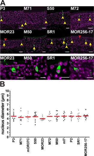
Fluorescent cells in the main olfactory epithelium of gene‐targeted mice. (A) Confocal images of coronal sections for eight selected strains sorted by average cell numbers: from P3, low, to MOR256‐17, high. The upper two rows show OSNs that are either counted (yellow arrows and arrowheads) or excluded from counting (red arrowheads). The bottom row shows magnified images of selected OSNs (yellow arrows). Intrinsic fluorescence in green, DAPI staining in magenta. (B) Nucleus diameter used for Abercrombie correction for the core set of 11 strains, measured with 10 single cells each. Scale bars = 20 μm in A, upper two rows, 10 μm in A, bottom row.

As an OSN that is cut in half and split over two consecutive 12‐μm sections can be counted twice, these raw cell counts represent an overestimate of the true OSN numbers. In order to obtain a closer approximation of true OSN numbers, we performed an Abercrombie correction (Abercrombie, 1946). We found that among the core set of 11 strains, fluorescent OSNs have a similar nucleus diameter (one‐way analysis of variance [ANOVA], P = 0.87) (Table 2, Fig. 1B): the average nucleus diameter is 4.42 μm ± 0.72, resulting in an average Abercrombie factor of 12/(12+4.42) = 0.73. We corrected the OSN counts with the Abercrombie factor specific for that strain. For the four additional strains with targeted mutations at the M71 locus, we used the Abercrombie factor of the M71‐IRES‐tauGFP strain.

Table 2.

Abercrombie Correction; Nucleus Diameter of OSNs

Strain name	Abbreviation	Nucleus diameter (μm)	Standard deviation (± μm)	Correction
P3‐IRES‐tauGFP	P3	4.51	0.80	0.73
M71‐IRES‐tauGFP	M71	4.26	1.05	0.74
mOR37C‐IRES‐tauGFP	mOR37C	4.39	0.62	0.73
S50‐IRES‐tauGFP	S50	4.40	0.91	0.73
MOR23‐IRES‐tauGFP	MOR23	4.00	0.39	0.75
M72‐IRES‐tauGFP	M72	4.47	0.74	0.73
M50‐IRES‐GFP‐IRES‐taulacZ	M50	4.49	0.79	0.73
mI7‐IRES‐tauGFP	mI7	4.53	0.65	0.73
P2‐IRES‐tauGFP	P2	4.53	0.60	0.73
SR1‐IRES‐tauGFP	SR1	4.49	0.72	0.73
MOR256‐17‐IRES‐tauGFP	MOR256‐17	4.59	0.58	0.72
β2AR→M71‐IRES‐tauGFP		4.26	1.05	0.74
RFP→M71iM71iGFP		4.26	1.05	0.74
M71‐IRES‐tauYFP		4.26	1.05	0.74
M71‐IRES‐tauRFP2		4.26	1.05	0.74

For each strain of the core set of 11 gene‐targeted strains, the average nucleus diameter and standard deviation are given, and the resulting Abercrombie correction factor.

Cell counts

Figure 2A shows the numbers of fluorescent cells in the core set of 11 strains representing the 11 gene‐targeted OR genes after Abercrombie correction. The OSN numbers for the strains PD21 are, from low to high: P3 (2,236 ± 247 cells), M71 (2,419 ± 484), mOR37C (2,660 ± 175), S50 (3,289 ± 503), MOR23 (4,446 ± 327), M72 (5,265 ± 906), M50 (6,716 ± 648), mI7 (9,892 ± 1,852), P2 (13,975 ± 1,982), SR1 (23,846 ± 1,706), and MOR256‐17 (37,023 ± 6,318). The average OSN number thus has a range of 17‐fold across these 11 OR‐tagged strains. Importantly, the spread within a given OR‐tagged strain is fairly small (see also below, coefficient of variation).

Figure 2.

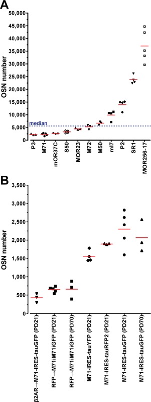
Numbers of fluorescent cells in OR‐IRES‐marker strains. (A) Average OSN number of the core set of 11 gene‐targeted strains at PD21. A symbol represents a single mouse. The blue line indicates the median of 5,983. (B) Average OSN number for strains with gene‐targeted mutations in the M71 locus at PD21 or PD70. The five mice of M71‐IRES‐tauGFP at PD21 in (B) are the same as in (A).

Figure 2B shows numbers of fluorescent cells in four other strains with mutations in the M71 gene: β2AR→M71‐IRES‐tauGFP (460 ± 131), RFP→M71iM71iGFP (650 ± 77), M71‐IRES‐tauYFP (1,558 ± 156), and M71‐IRES‐tauRFP2 (1,893 ± 14). There is no significant difference (t‐test, P = 0.21) in OSN numbers between M71‐IRES‐tauGFP and M71‐IRES‐tauRFP2 (red fluorescent protein), indicating a similar probability of OR gene choice and sensitivity of detection of intrinsic fluorescence. The OSN number in M71‐IRES‐tauYFP mice (yellow fluorescent protein) is lower than in M71‐IRES‐tauGFP mice (t‐test, P = 0.022) and M71‐IRES‐tauRFP2 mice (t‐test, P = 0.015), reflecting a possible difference in probability of OR gene choice and/or in sensitivity of detection of intrinsic fluorescence. OSN numbers are decreased in mutations in which the M71 coding region is replaced by that of the β2‐adrenergic receptor (β2AR→M71‐IRES‐tauGFP) (t‐test, P < 0.0001) or in which M71 translation is decreased by an IRES‐mediated knockdown (hypomorph, RFP→M71iM71iGFP) (t‐test, P = 0.0007). There are 2,067 ± 441 OSNs in M71‐IRES‐tauGFP mice (n = 3) at PD70, which is not significantly different (t‐test, P = 0.52) from PD21. For the hypomorph there is no difference either between PD21 and three mice at PD70 (660 ± 248 cells) (t‐test, P = 0.93).

Interleaved sampling

The availability of full cell counts provides a unique opportunity to determine exactly the error that would have been introduced by interleaved sampling. Partial cell counts are typically reported in the literature, because of the time and effort required to make full cell counts. We generated n virtual datasets corresponding to nth section sampling for the core set of 11 strains (Fig. 3A); for instance, we generated 10 virtual datasets consisting of cell counts in each 10th section. For each dataset, the cell counts were summed and multiplied by the sampling interval; in this example, multiplied by 10. The error produced by interleaved sampling can then be calculated by comparing the summed counts of a virtual dataset to the original, full cell count. The error and SD increase rapidly with decreased sampling interval, and are higher for strains with low OSN numbers such as P3‐IRES‐tauGFP than for strains with high OSN numbers such as MOR256‐17‐IRES‐tauGFP (Fig. 3B).

Figure 3.

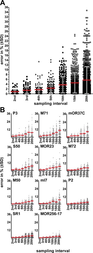
Effect of sampling interval. (A) Average percentage of difference (error) in interleaved sampling compared to the “count every cell” approach (±SD). Errors for all tauGFP strains for each sampling interval were pooled to calculate the averages. A symbol represents a single virtual sampling set. (B) Error of cell counts by sampling interval for GFP‐expressing strains sorted by average OSN number, from P3, low, to MOR256‐17, high. A symbol represents a single virtual sampling set.

Coefficient of variation

The coefficient of variation (CV) is the ratio of SD over average. Among the core set of 11 strains, the CV for the OSN number within a strain ranges over a factor of 3.2‐fold, from 0.066 (mOR37C‐IRES‐tauGFP) to 0.21 (M71‐IRES‐tauGFP), but there is no correlation with average OSN number (Fig. 4): MOR23‐IRES‐tauGFP has a similarly low CV (0.074) as SR1‐IRES‐tauGFP (0.072), but the number of OSNs is 5.5‐fold lower. Conversely, M72‐IRES‐tauGFP has a CV (0.172) similar to that of MOR256‐IRES‐tauGFP (0.171), but the number of OSNs is 7‐fold lower. Thus, the probability of OR gene choice appears to be more constant for certain OR genes than for others. From a practical experimental viewpoint, FP‐tagged strains with a higher stability in OSN population size (a lower CV) such as MOR23‐IRES‐tauGFP are easier to study quantitatively.

Figure 4.

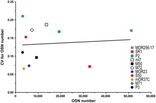
Coefficient of variation (CV). CV for average OSN number of the 11 GFP strains shows that there is no correlation between average OSN number and CV. The line is best modeled by y = 3.1*10^‐7x + 0.13 (r² = 0.008, P = 0.79).

Cell counts along the anterior–posterior dimension

OSNs expressing a given OR gene display a characteristic spatial pattern across the MOE (Ressler et al., 1993; Miyamichi et al., 2005). The availability of full cell counts enables us to plot cell count per 12‐μm section along the anterior–posterior dimension of the MOE. Figure 5A shows the diversity of these plots, reflecting the multitude of spatial expression patterns. OR genes expressed dorsally such as M71 and MOR23 have a relatively even distribution, starting far anteriorly. The relatively even distribution of M71 is maintained in mutations in which the M71 coding region is replaced by that of the β2‐adrenergic receptor (β2AR→M71‐IRES‐tauGFP) or in which M71 translation is decreased by an IRES‐mediated knockdown (RFP→M71iM71iGFP) (Fig. 5B). But other OR genes show a single peak (MOR256‐17) or two peaks (SR1) along the anterior–posterior dimension (Fig. 5C). These peaks compromise the accuracy of comparing partial cell counts among individual mice, due to the lack of fiduciary points.

Figure 5.

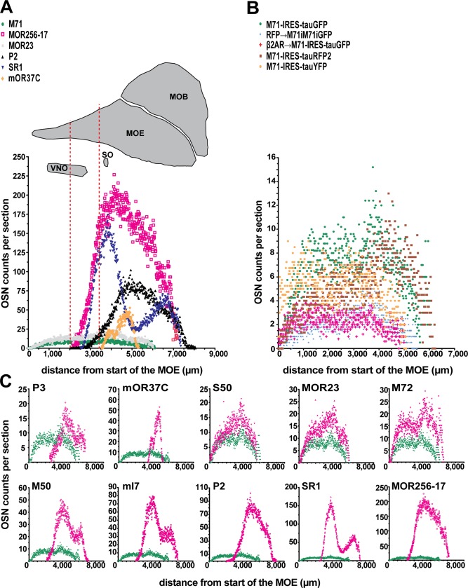
OSN counts across the anterior–posterior dimension of the main olfactory epithelium. (A) Average OSN counts per section. The dotted red lines indicate two reference positions in a sagittal view of a mouse head. Strains were chosen for showing the diversity in expression per section. Cells in the septal organ are not included in these counts. (B) Average OSN counts per section for strains with mutations in the M71 gene. (C) Average OSN counts per section of (tau)GFP‐expressing strains (magenta) compared to M71‐IRES‐tauGFP (green), sorted by average OSN number from P3, low, to MOR256‐17, high. The strains display a multitude of spatial expression patterns/zones.

Total glomerular volume

Next we studied the glomeruli that correspond to an FP‐tagged OSN cell population, again based on intrinsic fluorescence and using the same series of coronal sections as for counting OSNs in the MOE (Fig. 6A). The area of a glomerulus displaying intrinsic fluorescence can be calculated by confocal imaging in z‐stacks, but this procedure for determining glomerular volume is very time‐consuming. Therefore, we computed glomerular volume by reconstruction. The sum of the reconstructed volumes of all fluorescently labeled glomeruli in a mouse is the TGV.

Figure 6.

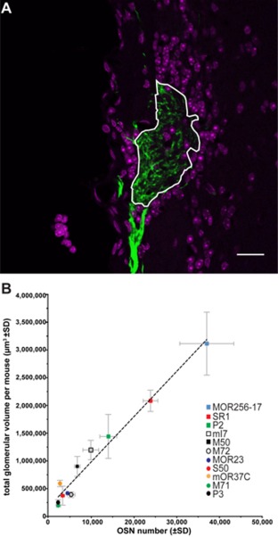
Glomerular volume and correlation with OSN numbers. (A) Confocal image of an M71‐IRES‐tauGFP glomerulus. Green, intrinsic fluorescence; magenta, DAPI. The area framed in white is measured as the cross‐sectional area. (B) TGV per strain at PD21 correlates strongly and linearly to the OSN number (r² = 0.97, P ≤ 0.0001) in the core set of 11 strains. The curve is best modeled by y = 81.55x + 168,700. A symbol represents a single strain. Scale bar = 20 μm in A.

We found a strong linear correlation between OSN number and TGV among the 54 mice of the core set of 11 gene‐targeted strains analyzed at PD21 (Fig. 6B): r² = 0.97 at P ≤ 0.0001 with an intercept of the Y axis at 168,700 μm³ and a slope of 81.55. The practical implication of this linear correlation is that TGV, which is relatively easy to compute, can be used to estimate accurately OSN number, which is far more time‐consuming to determine.

Fluorescent pixel density in glomeruli

Finally, we determined the fluorescent pixel density of labeled glomeruli in the confocal images used for the reconstruction of glomerular volume. Fluorescent pixel density is an estimate of the density of OSN axon branches and axon terminals within a glomerulus. We found a relatively constant density of ∼0.80 across the strains; a density of 0.80 means that 80% of the pixels in the glomerulus display fluorescence above background (Fig. 7A). The S50 glomeruli have a value of 0.56. It turns out that the lateral S50 glomeruli (Fig. 7B) have a value of 0.40 (Fig. 7D), but the medial S50 glomeruli (Fig. 7C) have a normal value of 0.79 (Fig. 7D). Explanations could be that lateral S50 glomeruli are not yet fully mature by PD21, that they have indeed a lower density of OSN axon branches and terminals, or that they are coinnervated by axons from OSNs expressing another OR.

Figure 7.

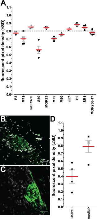
Fluorescent pixel density in glomeruli. (A) The ratio of fluorescent pixels to all pixels in the glomerular area is ∼0.8 in all strains (ANOVA, F = 21.50, P < 0.0001), except for S50‐IRES‐tauGFP. A symbol represents a single mouse. Strains are sorted by average OSN number from P3, low, to MOR256‐17, high. (B) Example of a lateral S50‐IRES‐tauGFP glomerulus illustrates its lower fluorescent pixel density. Green, intrinsic fluorescence; white, DAPI. (C) Example of a medial S50‐IRES‐tauGFP glomerulus. (D) Ratios of axonal density for lateral versus medial S50‐IRES‐tauGFP glomeruli (±SD) show that only the lateral glomeruli have a lower fluorescent pixel density. A symbol represents the average of glomeruli in both bulbs of an individual mouse. Scale bars = 20 μm.

DISCUSSION

The introduction of a genetic strategy based on an IRES and the axonal marker tauβ‐galactosidase in 1996 has become a standard approach for anatomical analyses of spatial patterns of OR gene expression in the MOE and of their corresponding glomeruli in the olfactory bulb (Mombaerts et al., 1996; Mombaerts, 2006). The axonal marker tauGFP and variants tauYFP and tauRFP2 are more versatile than taulacZ: they facilitate imaging of glomeruli by confocal microscopy and two‐photon microscopy (Potter et al., 2001), they enable physiological studies (Bozza et al., 2002; Grosmaitre et al., 2006, 2009; Omura et al., 2014), they allow for flow‐cytometric cell sorting (Khan et al., 2011), and the manual picking of single cells expressing a given OR gene (Li et al., 2004; Fuss et al., 2013). We therefore examined mice of strains with a gene‐targeted mutation in an OR gene that generates a fluorescent protein. To facilitate volumetric measurements of glomeruli in the same series of coronal sections as were used for cell counting in the MOE, our analyses are based on the relatively simple detection method of intrinsic fluorescence by confocal microscopy.

A lingering belief is that each of the ∼1,100 OR genes is expressed in a similar number of OSNs. We found a range of 17‐fold between the smallest OSN population (P3‐IRES‐tauGFP) and the largest OSN population (MOR256‐17‐IRES‐tauGFP) at PD21, in our 1% sample of the ∼1,100 OR genes. We suggest to take provisionally the median of 5,983 as the OSN number for the average OR gene at PD21. In turn, this number of 5,983 results in an estimate of ∼6.6 million OSNs expressing any of the 1,100 OR genes in a mouse at PD21 in this mixed 129 × B6 background. If not all 1,100 OR genes are expressed in OSNs, the total number of OR‐expressing OSNs from these estimates will be lower. Our estimate is lower than the estimate of ∼9,400 OSNs expressing on average a given OR gene in the ∼10 million mature, OMP‐expressing OSNs in 8‐week‐old C57BL/6J mice (Kawagishi et al., 2014). But the age difference of 3 versus 8 weeks is substantial, and the fraction of OMP‐expressing OSNs that does not express an OR gene is not known.

We reported a broad range of NanoString counts for OR mRNAs in wildtype C57BL/6 mice: 92% of OR genes have NanoString counts within a 32‐fold range (Khan et al., 2011, 2013). These NanoString counts are not directly translatable into OSN numbers, for several reasons (Khan et al., 2013). The probabilities of OR gene choice appear to differ widely across the OR gene repertoire, and the mechanistic basis of these differences remains to be clarified. As OSN survival and turnover are likely dependent on the odorant composition of the inhaled air, we provide information in the Materials and Methods about the type of caging, food, and bedding used. It is conceivable that OSN counts may be different in mice that are housed in other types of caging (such as open cages versus individually ventilated cages) or given other food and bedding.

Our empirical, “count every cell” strategy generates total cell counts, which appear rarely in the literature, presumably due to the amount of effort that is required. A rare example of total cell counts can be found in Royal and Key (1999). Counting cells expressing the OR gene P2 by X‐gal histochemistry in P2‐IRES‐tauLacZ mice but without Abercrombie correction, Royal and Key reported 8,286 labeled cells at PD14.5 and 13,729 at 12 weeks, whereas we found 13,975 ± 1,982 labeled cells at PD21 in P2‐IRES‐tauGFP mice.

From our complete datasets we generated n virtual datasets, as if we had counted cells on every nth section, in n successive datasets. We were thus able to calculate exactly the error that is produced by interleaved sampling. We found that, as expected, the SD increases rapidly with increasing interval, reaching ±5.63 for every 20th section (average error 5.75%). The information we provide about the 11 strains enables now to define a priori the acceptable error for studies in which cell counts are compared between experimental conditions.

Counting OSNs expressing a given OR gene or fluorescent protein remains a manual enterprise: a patient and astute observer sits at the microscope and counts cells one by one. No reliable automated methods have been developed thus far. As a surrogate for cell counting, we propose to compute TGV, which takes far less effort. Reconstruction of these volumes can be done readily by measuring the glomerular area in the middle optical section of physical sections under a confocal microscope. The very strong linearity of the correlation between OSN number and TGV, over a range of 17‐fold, implies that estimates of OSN numbers can be read out from the curve we provide. Our findings are consistent with the linear correlation that has been described between partial cell counts in the MOE of M71‐IRES‐taulacZ mice and the average largest cross‐sectional area of an M71 glomerulus (Jones et al., 2008).

OSN number estimates derived from TGV may be sufficiently accurate, depending on the goals of the study and the number of mice that need to be analyzed. The linearity of this correlation is not entirely surprising, but also not obvious. One could have expected that at low and high OSN numbers the curve would flatten out ‐ in particular at lower OSN numbers, as a fixed minimum volume of a glomerulus could be occupied by nonaxonal structures.

A limitation of our studies is that they are based on mice in the conventional mixed 129 × B6 background, which is currently the best practice. Backcrossing of the targeted mutations to C57BL/6 may help in reducing some of the variability. But as most of OR gene regulation takes place in cis, at the promoter level, the regions around the targeted OR locus will always be of 129 origin ‐ in fact, they will continue to be the nucleotide sequences that were present in the genome of the original embryonic stem cell in which the targeted mutation was introduced by homologous recombination. Thanks to the emergence of the new genetic manipulation technology of CRISPR/Cas9, we expect that some of these FP‐tagged mutations will be made or remade directly in a C57BL/6 background. It will then also be possible to compare cell numbers between counting fluorescent cells in FP‐tagged strains with counting cells expressing the corresponding unmanipulated OR gene in wildtype C57BL/6 mice by RNA in situ hybridization.

In conclusion, the practical outcome of our empirical study is that TGV is a highly reliable indicator of OSN number.

CONFLICT OF INTEREST

The authors declare no conflicts of interest.

ROLE OF AUTHORS

All authors had full access to all the data in the study and take responsibility for the integrity of the data and the accuracy of the data analysis. Study concept and design: OCB, MK, PM. Acquisition of data: OCB. Statistical analysis: OCB. All authors contributed to the analysis and interpretation of data. Drafting of the article: PM. Obtained funding: PM.

LITERATURE CITED

- Abercrombie, M. 1946. Estimation of nuclear population from microtome sections. Anat Rec 94:239–247. [DOI] [PubMed] [Google Scholar]
- Benes FM, Lange N. 2001. Two‐dimensional versus three‐dimensional cell counting: a practical perspective. Trends Neurosci 24:11–17. [DOI] [PubMed] [Google Scholar]
- Bozza T, Feinstein P, Zheng C, Mombaerts P. 2002. Odorant receptor expression defines functional units in the mouse olfactory system. J Neurosci 22:3033–3043. [DOI] [PMC free article] [PubMed] [Google Scholar]
- Bozza T, Vassalli A, Fuss S, Zhang JJ, Weiland B, Pacifico R, Feinstein P, Mombaerts P. 2009. Mapping of class I and class II odorant receptors to glomerular domains by two distinct types of olfactory sensory neurons in the mouse. Neuron 29:220–233. [DOI] [PMC free article] [PubMed] [Google Scholar]
- Buck L, Axel R. 1991. A novel multigene family may encode odorant receptors: a molecular basis for odor recognition. Cell 65:175–187. [DOI] [PubMed] [Google Scholar]
- Cummings DM, Belluscio L. 2010. Continuous neural plasticity in the olfactory intrabulbar circuitry. J Neurosci 30:9172–9180. [DOI] [PMC free article] [PubMed] [Google Scholar]
- Feinstein P, Mombaerts P. 2004. A contextual model for axonal sorting into glomeruli in the mouse olfactory system. Cell 117:817–831. [DOI] [PubMed] [Google Scholar]
- Feinstein P, Bozza T, Rodriguez I, Vassalli A, Mombaerts P. 2004. Axon guidance of mouse olfactory sensory neurons by odorant receptors and the β2 adrenergic receptor. Cell 117:833–846. [DOI] [PubMed] [Google Scholar]
- Fuss SH, Zhu Y, Mombaerts P. 2013. Odorant receptor gene choice and axonal wiring in mice with deletion mutations in the odorant receptor gene SR1 . Mol Cell Neurosci 56:212–224. [DOI] [PubMed] [Google Scholar]
- Grosmaitre X, Vassalli A, Mombaerts P, Shepherd GM, Ma M. 2006. Odorant responses of olfactory sensory neurons expressing the odorant receptor MOR23: a patch clamp analysis in gene‐targeted mice. Proc Natl Acad Sci U S A 103:1970–1975. [DOI] [PMC free article] [PubMed] [Google Scholar]
- Grosmaitre X, Fuss SH, Lee AC, Adipietro KA, Matsunami H, Mombaerts P, Ma M. 2009. SR1, a mouse odorant receptor with an unusually broad response profile. J Neurosci 29:14545–14552. [DOI] [PMC free article] [PubMed] [Google Scholar]
- Guena S. 2000. Appreciating the difference between design‐based and model‐based sampling strategies in quantitative morphology of the nervous system. J Comp Neurol 427:333–339. [PubMed] [Google Scholar]
- Guillery RW. 2002. On counting and counting errors. J Comp Neurol 447:1–7. [DOI] [PubMed] [Google Scholar]
- Jones SV, Choi DC, Davis M, Ressler KJ. 2008. Learning‐dependent structural plasticity in the adult olfactory pathway. J Neurosci 28:13106–13111. [DOI] [PMC free article] [PubMed] [Google Scholar]
- Kawagishi K, Ando M, Yokouchi K, Sumitomo N, Karasawa M. Fukushima N, Moriizumi T. 2014. Stereological quantification of olfactory receptor neurons in mice. Neuroscience 272:29–33. [DOI] [PubMed] [Google Scholar]
- Khan M, Vaes E, Mombaerts P. 2011. Regulation of the probability of mouse odorant receptor gene choice. Cell 147:907–921. [DOI] [PubMed] [Google Scholar]
- Khan M, Vaes E, Mombaerts P. 2013. Temporal patterns of odorant receptor gene expression in adult and aged mice. Mol Cell Neurosci 57:120–129. [DOI] [PubMed] [Google Scholar]
- Li J, Ishii T, Feinstein P, Mombaerts P. 2004. Odorant receptor gene choice is reset by nuclear transfer from mouse olfactory sensory neurons. Nature 428:393–399. [DOI] [PubMed] [Google Scholar]
- Miyamichi K, Serizawa S, Kimura HM, Sakano H. 2005. Continuous and overlapping expression domains of odorant receptor genes in the olfactory epithelium determine the dorsal/ventral positioning of glomeruli in the olfactory bulb. J Neurosci 25:3586–3592. [DOI] [PMC free article] [PubMed] [Google Scholar]
- Mombaerts P. 2006. Axonal wiring in the mouse olfactory system. Annu Rev Cell Dev Biol 22:713–737. [DOI] [PubMed] [Google Scholar]
- Mombaerts P, Wang F, Dulac C, Chao SK, Nemes A, Mendelsohn M, Edmondson J, Axel R. 1996. Visualizing an olfactory sensory map. Cell 87:675–686. [DOI] [PubMed] [Google Scholar]
- Omura M, Grosmaitre X, Ma M, Mombaerts P. 2014. The β2‐adrenergic receptor as a surrogate odorant receptor in mouse olfactory sensory neurons. Mol Cell Neurosci 58:1–10. [DOI] [PMC free article] [PubMed] [Google Scholar]
- Potter SM, Zheng C, Koos DS, Feinstein P, Fraser SE, Mombaerts P. 2001. Structure and emergence of specific olfactory glomeruli in the mouse. J Neurosci 21:9713–9723. [DOI] [PMC free article] [PubMed] [Google Scholar]
- Ressler KJ, Sullivan SL, Buck LB. 1993. A zonal organization of odorant receptor gene expression in the olfactory epithelium. Cell 73:597–609. [DOI] [PubMed] [Google Scholar]
- Ressler KJ, Sullivan SL, Buck LB. 1994. Information coding in the olfactory system: evidence for a stereotyped and highly organized epitope map in the olfactory bulb. Cell 79:1245–1255. [DOI] [PubMed] [Google Scholar]
- Richard MB, Taylor SR, Greer CA. 2010. Age‐induced disruption of selective olfactory bulb synaptic circuits. Proc Natl Acad Sci U S A 107:15613–15618. [DOI] [PMC free article] [PubMed] [Google Scholar]
- Rolen SH, Sacedo E, Restrepo D, Finger TE. 2014. Differential localization of NT‐3 and TrpM5 in glomeruli of the olfactory bulb of mice. J Comp Neurol 522:1929–1940. [DOI] [PMC free article] [PubMed] [Google Scholar]
- Royal SJ, Key B. 1999. Development of P2 olfactory glomeruli in P2 internal ribosome entry site taulacZ transgenic mice. J Neurosci 19:9856–9864. [DOI] [PMC free article] [PubMed] [Google Scholar]
- Schaefer ML, Finger TE, Restrepo D. 2001. Variability of position of the P2 glomerulus within a map of the mouse olfactory bulb. J Comp Neurol 436:351–362. [PubMed] [Google Scholar]
- Schoenfeld TA, Knott TK. 2004. Evidence for disproportionate mapping of olfactory airspace onto the main olfactory bulb of the hamster. J Comp Neurol 476:186–201. [DOI] [PubMed] [Google Scholar]
- Schmitz C, Hof PR. 2005. Design‐based stereology in neuroscience. Neuroscience 130:813–831. [DOI] [PubMed] [Google Scholar]
- Strotmann J, Conzelmann S, Beck A, Feinstein P, Breer H, Mombaerts P. 2000. Local permutations in the glomerular array of the mouse olfactory bulb. J Neurosci 20:6927–6938. [DOI] [PMC free article] [PubMed] [Google Scholar]
- Vassalli A, Rothman A, Feinstein P, Zapotocky M, Mombaerts P. 2002. Minigenes impart odorant receptor‐specific axon guidance in the olfactory bulb. Neuron 35:681–696. [DOI] [PubMed] [Google Scholar]