Anthropic Correction of Information Estimates and Its Application to Neural Coding

Abstract

Information theory has been used as an organizing principle in neuroscience for several decades. Estimates of the mutual information (MI) between signals acquired in neurophysiological experiments are believed to yield insights into the structure of the underlying information processing architectures. With the pervasive availability of recordings from many neurons, several information and redundancy measures have been proposed in the recent literature. A typical scenario is that only a small number of stimuli can be tested, while ample response data may be available for each of the tested stimuli. The resulting asymmetric information estimation problem is considered. It is shown that the direct plug-in information estimate has a negative bias. An anthropic correction is introduced that has a positive bias. These two complementary estimators and their combinations are natural candidates for information estimation in neuroscience. Tail and variance bounds are given for both estimates. The proposed information estimates are applied to the analysis of neural discrimination and redundancy in the avian auditory system.

I. Introduction

Information theoretic approaches play an important role in sensory neuroscience where the estimation of the mutual information (MI) between stimuli and responses has provided a model-independent measure of neural discrimination [1], [2]. In this context, MI has been used for three different purposes. First, in its most direct use, MI can be used to determine which features of the stimulus are encoded in the neural response, and thus provides an attractive alternative to explicitly modeling these systems. By comparing MI measures obtained from different sets of stimuli or even for particular stimuli, one can determine which stimulus features are preferentially encoded in neural responses. Many approaches of this type have been developed; see, e.g., [3]. For example, behaviorally relevant natural sounds have been shown to evoke higher information rates in comparison to matched synthetic sounds in both frogs [4] and birds [5]. The second application is in the determination of the nature of the neural code. For this purpose, the MI is compared for different decoders of the neural response [6]. For example, one could compare a decoder that just counts the number of neuronal spiking events in a time window (a rate code) to a decoder that takes into account the timing of those events (a temporal code). The nature of the neural code can also be examined for neuronal ensembles, for example to determine whether temporal patterns across neurons play a particular role. The third application is in the assessment of the efficiency of the neural representation. At the level of single neurons, the efficiency of the code can be determined by comparing the actual MI observed in the experiment to the “channel capacity” obtained by fixing the conditional distribution as observed in the experiment, but maximizing over the input distribution; see, e.g., [4]. The efficiency of the neural code can also be assessed in information maximization problems where the actual neural representation is compared to theoretically derived optima. For example, wind direction in the cricket cercal system has been shown to be best represented by truncated cosine tuning curves [7] and the early stages of the visual system perform a spatio–temporal decorrelation that has been shown to maximize neural efficiency in information-theoretic terms [8]. One of the most interesting new applications in the assessment of neural efficiency is the consideration of redundancy in the responses of a population of neurons [9]–[12]. On the one hand, different neurons may react similarly to certain stimulus features and the code can be redundant [11]. On the other hand, neurons could represent independent information in a synergistic fashion [10]. Finally, redundancy can change in a processing stream revealing the nature of the computation occurring across levels [12].

Although the use of information theory in neuroscience could already be considered a success, one of the principal factors that limit its applicability is the curse of dimensionality: the stimulus space being analyzed by sensory systems is very large and the neural representation can involve millions of neurons with neural signals that can be precise on a millisecond time scale. Although experimental techniques for recording neural activity are improving, recordings of single neurons that last more than one day are still extremely rare. The major problem in applying information theory to neuroscience is therefore one of data limitation. This issue has been addressed before with a focus on how to obtain estimates of MI with smaller error and bias (see, e.g., [13] for an overview) and on how to reduce the dimensionality of the neural response to obtain lower bounds on the MI [6]. However, two issues have not been addressed explicitly or extensively in previous work: the effect of undersampling the stimulus space and the lack of good upper bounds for the MI. In particular, the calculation of redundancy in stimulus ensembles using lower bound estimates could lead to significant overestimation of redundancy.

In this paper, we propose a novel estimator that partially addresses these shortcomings. Let us first consider the problem of undersampling the stimulus space. Indeed, for many of the existing data sets in sensory neuroscience, there are relatively few stimuli, and relatively many response measurements for each stimulus. Here, unless additional assumptions are made, any naive information estimate is upper bounded by the logarithm of the number of stimuli that were presented during the experiment, and MI estimates saturate (e.g., [14] and [15]). We are thus confronted with a saturating lower bound. To avoid this effect, the number of tested stimuli must increase exponentially with the MI. In classical single-neuron problems, this may be less of an issue, but we anticipate that it will become much more limiting in the analysis of neuronal populations.

As a case in point, consider a neuron population of size M: The MI between the stimulus and all M neurons can increase linearly in M [namely, when each neuron describes a separate (independent) component of the stimulus], and hence, the number of stimuli that need to be used can behave like # stimuli ≈ 2^MI₀, that is, exponentially in the population size (where is I₀ an appropriate constant). To deal with this issue, we present a novel estimate of the MI referred to as the anthropic correction. We will show that this estimator is guaranteed to have a nonnegative bias, and in this sense serves as an “upper bound” to the true MI. We also argue that together, lower and upper bounds can better characterize MI, yielding better estimates of MI and redundancy, in particular as the number of neurons in the considered population becomes large.

In Section II, we define the proposed estimator and derive its fundamental properties. Sections III and IV present applications of the proposed estimator to measurement data.

A. Notation

Throughout the paper, capital letters such as X will denote random variables and lower case letters such as x their realizations. The notation p_X(x) will denote the probability mass function of the random variable X, taking values in a set 𝒳 of cardinality |𝒳|. When no confusion arises, we will use the shorthand p(x). We will mostly use the standard terminology as in [16]; thus, for example, we will use I(X; Y) to denote the MI between the random variables X and Y.

II. Anthropic Correction of Information Estimates

In much of the literature, information estimates are considered for the scenario where N independent and identically distributed (i.i.d.) samples of a distribution p(x, y) are available. However, the i.i.d. assumption does not seem to be a good match for many standard data sets in neuroscience. Rather, it is often the case that for a relatively small set of different stimuli, ample response data is available. To model this scenario, in this paper, we consider the following: Two random variables X and Y take values in discrete and finite sets 𝒳 and 𝒴, respectively, and are distributed according to a distribution p(x, y). We suppose there are K samples of X available, denoted by {x₁, x₂, …, x_K}, and for each of these K samples, there are n samples of Y available, denoted by {y_{k, j}}, for k = 1, 2, …, K and j = 1, 2, …, n. The task is to estimate the MI I(X; Y). Motivated by this setting, in this paper, we study properties and applications of the following novel estimator of MI.

Definition 1

The anthropically corrected information estimate is defined as

$${Î}_{\alpha }^{(K,n)}=\frac{1}{K}\sum _{k=1}^K{𝔻}_{KL}(\hat{p}(y|x=x_k)\Vert {\hat{p}}_{k,\alpha }(y))$$ (1)

where

$${\hat{p}}_{k,\alpha }(y)=\frac{1-\alpha }{K}\sum _{i=1}^K\hat{p}(y|x=x_i)+\frac{\alpha }{K-1}\sum _{j=1,j\ne k}^K\hat{p}(y|x=x_j).$$ (2)

where p̂(y|x = x_j) is the histogram (plug-in) estimate of the conditional distribution p(y|x = x_j) based on the n available samples.

We will refer to the estimate ${Î}_0^{(K,n)}$ as the plug-in (or naive) estimate, and to the estimate ${Î}_1^{(K,n)}$ as the full anthropic correction.¹

Remark 1

It is also interesting to consider more general divergence estimators, some examples being [18] and [19]. In particular, this would permit to apply the proposed estimator to the case where the random variable Y is continuous valued. However, this is outside the scope of this paper.

A. Basic Properties

We start by providing two useful properties of the proposed estimator, summarized in the following lemma.

Lemma 1

The anthropically corrected information estimate satisfies the following properties:

1. it is nonnegative and upper bounded as follows:

   $$0\le {Î}_{\alpha }^{(K,n)}\le {\text{log}}_{2}K+{\text{log}}_2\frac{1}{1-\alpha };$$ (3)
2. it is a nondecreasing function of α; more precisely

   $${Î}_{\alpha }^{(K,n)}\le (1-\frac{\alpha \prime -\alpha }{K-1+\alpha \prime }){Î}_{\alpha \prime }^{(K,n)},\hspace{1em}\text{for}\alpha \le \alpha \prime .$$ (4)

A proof of this lemma is given in Appendix I.

Remark 2

The first property illustrates the motivation for the anthropic correction: The plug-in information estimate (α = 0) is upper bounded by log₂ K. When K is small but the true value of I(X; Y) is large, this upper bound introduces a significant negative bias.

B. Bias Properties for Fixed K

The proposed estimator is interesting for finite K. In particular, while the “plug-in” estimate (α = 0) has a negative bias, we will now show that in an appropriate sense, the proposed (full) anthropic correction (α = 1) has a positive bias.

To make this precise, we will assume that K i.i.d. samples from the distribution p(x) are given, denoted by {x₁, x₂, …, x_K}. For each sample x_k, we obtain n i.i.d. samples y_{k, j}, for j = 1, 2, …, n, drawn according to p(y|x_k). Letting n → ∞, we obtain exact estimates of the conditional distributions for each sample x_k, which obviously still does not give an exact estimate of the MI I(X; Y) since there are only K samples of the random variable X. In order to state the main result of this section, let us now define the quantity

$${Î}_{\alpha }^{(K)}=\frac{1}{K}\sum _{k=1}^K𝔻(p(y|x_k)\Vert p_{k,\alpha }(y)).$$ (5)

Note that this is the limit of ${Î}_{\alpha }^{(K,n)}$ as n → ∞. With this, we have the following theorem.

Theorem 1

For any integer K > 0, we have that

$$𝔼\left[{Î}_0^{(K)}\right]\le I(X;Y)\le 𝔼\left[{Î}_1^{(K)}\right]$$ (6)

i.e., asymptotically in n, the plug-in information estimate has a negative bias, and the (full) anthropic correction has a positive bias.

A proof of this theorem is given in Appendix II.

This theorem suggests that practically interesting estimators can be obtained by selecting the anthropic parameter α appropriately: by the intermediate value theorem, for each distribution p(x, y) and every positive integer K, there exists a value of α for which ${Î}_{\alpha }^{(K)}$ is unbiased. Universally good choices of α (as a function of K and perhaps some coarse information about p(x, y), such as the first few moments of this distribution) are therefore of interest, though outside of the scope of this paper.

The theorem also suggests estimators of the form

$${Î}^{(K)}(\beta )=\beta {Î}_0^{(K)}+(1-\beta ){Î}_1^{(K)}$$ (7)

again because the intermediate value theorem establishes that there exists a value of β for which Î^(K)(β) is unbiased. By analogy, it is of interest to derive universally good choices of the parameter β, based on coarse information about p(x, y).

Remark 3

We note that no universally unbiased estimate of the MI exists for finite K, even when n → ∞. For a very simple proof of this fact, see [13].

Remark 4

The bias of entropy, divergence, and information estimators in the neuroscience context has been discussed widely in the literature, including [13], [6] and [20]–[23]. Many bias correction techniques were proposed. The most popular may be the “jackknife”; see, e.g., [24].

Remark 5

It is simple to show that for the setup considered, with i.i.d. samples, the bias of the estimator ${Î}_{\alpha =1}^{(K,n)}$ is infinite as long as n is finite. This is because for finite n, there is a nonzero probability that there is a value of y for which for some k, we have p̂(y|x_k) > 0 but for all ℓ ≠ k, we have p̂(y|x_ℓ) = 0, making ${Î}_{\alpha =1}^{(K,n)}$ infinite. To show that this does not negate the usefulness of the proposed anthropic correction, we provide a tail bound in the next section.

Remark 6

Note that for the plug-in estimator, it is not true that $𝔼[{Î}_0^{(K,n)}]\le I(X;Y)$ for finite n. To see this, consider a model where p(x, y) = p(x)p(y) and thus, I(X; Y) = 0. However, with positive probability, ${Î}_0^{(K,n)}>0$, which implies that $𝔼[{Î}_0^{(K,n)}]>0$.

C. Tail and Variance Properties for Fixed K

In this section, we continue with the modeling assumptions introduced in Section II-B. For a fixed number K of samples of the random variable X,, it is straightforward to see that as n tends to infinity, ${Î}_{\alpha }^{(K,n)}$ tends to ${Î}_{\alpha }^{(K)}$. A more interesting question concerns the characterization of this convergence, and in this section, we provide two results. First, we study the tail behavior, then the variance. While tighter tail bounds can likely be established, perhaps along the lines of the analysis in [25], our main interest lies in the fact that our bound also applies to the case of the full anthropic correction (α = 1).

To express our bounds, we introduce the following notation:

$$D_{\text{max},\alpha }=\underset{k}{\text{max}}𝔻(p(y|x_k)\Vert p_{k,\alpha }(y)).$$ (8)

Then, we have the following tail bound.

Theorem 2

Assume p(y|x) > 0, for all y and x. For any 0 < ε < 1/2 and any 0 ≤ α ≤ 1 for which D_max,α < ∞, we have

$$\mathbb{P}\left(\right|{Î}_{\alpha }^{(K,n)}-{Î}_{\alpha }^{(K)}|>\epsilon (D_{\text{max},\alpha }+6))\le \frac{C_1}{n{\epsilon }^2}$$ (9)

where C₁ is a constant independent of n and ε.

The proof of this theorem is given in Appendix III.

For the variance, we obtain the following.

Theorem 3

Assume p(y|x) > 0, for all y and x. For any 0 ≤ α < 1 for which D_max,α < ∞, we have

$$𝔼\left[{({Î}_{\alpha }^{(K,n)}-{Î}_{\alpha }^{(K)})}^2\right]\le \frac{C_2}{\sqrt{n}}$$ (10)

where C₂ is a constant independent of n.

The proof of this theorem is given in Appendix III.

Remark 7

Note that for α = 1, no variance bound can be given because for any finite n, there is a strictly nonzero probability that ${Î}_1^{(K,n)}=\infty$.

D. Convergence Properties as K → ∞

Continuing again in the framework of the modeling assumptions introduced in Section II-B, we end the discussion by stating that as K → ∞, the proposed estimator ${Î}_{\alpha }^{(K)}$ tends to the true information I(X; Y) almost surely, irrespective of the value of α. To see this, it suffices to observe that 𝔼[p_k,α(y)] = p(y), for all y ∈ 𝒴, where the expectation is over the i.i.d. selection of K samples from p(x). Since moreover, p_k,α(y) is a sum of i.i.d. random variables, it follows that it converges almost surely to p(y) for all y ∈ 𝒴. A more precise characterization is beyond the interest of this study, which concerns the case of small K, where the proposed estimator appears to be most useful.

E. Numerical Illustration

We provide a simple numerical illustration to give a sense of the anthropic correction: let S be uniformly distributed over {0, 1, 2, …, M − 1}, and R be given by R = S + Z, where addition is modulo M, and Z is distributed according to

$$p(z)=\frac{1-\epsilon }{N},\hspace{1em}\text{for}z=0,1,\dots ,N-1$$ (11)

and

$$p(z)=\frac{\epsilon }{M-N},\hspace{1em}\text{for}z=N,N+1,\dots ,M-1.$$ (12)

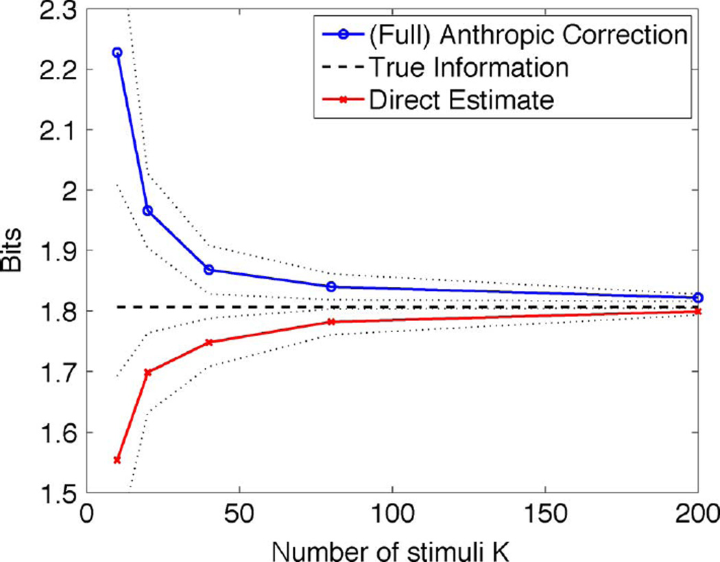
K i.i.d. samples from the distribution of S were taken. Fig. 1 shows ${Î}_{\alpha }^{(K,n)}$ for α = 0 (labeled “direct estimate”) and for α = 1 [labeled “(full) anthropic correction”] for various values of K, with n = 10⁴. Each point in the plot corresponds to 50 independent trial runs. The solid lines are the means and the dotted lines the standard deviations over these experiments. The figure illustrates the somewhat symmetric behavior, in terms of positive and negative biases, of the anthropic correction and the naive estimate, respectively.

Fig. 1.

Discrete example with M = 50, ε = 0.05, and N = 11. This figure shows the situation where for each tested stimulus, the response distribution was estimated from 10⁴ samples.

III. Application I: Information Estimation

A. Stimulus-Response Information Estimation

As a first application of the proposed novel estimator, we consider the basic problem of estimating the MI between the stimulus and the response of a single neuron. This is a classical problem and has been extensively studied in the literature, as discussed in Section I.

Specifically, we consider data from recordings in the songbird analog of auditory cortex, a forebrain area called field L. Neural responses in field L were obtained from urethane anesthetized male zebra finches in response to the playback of a representative set of 20 different adult zebra finch songs. Each song lasted approximately 2 s. Ten trials of neural responses were obtained for each song. These trials are called spike trains because they consist of individual spiking events (action potentials). Experimental details and examples of raw data traces can be found in [5]. In this paper, we are reporting the results from 66 neurons recorded in 12 birds.

Obviously, for our experiments, the true MI is not known. Instead, we will consider as the “ground truth” and baseline for comparisons the MI corresponding to an inhomogeneous gamma model of the observed spiking activity. The gamma information involves modeling the neuronal responses as inhomogeneous gamma processes [5]. For this modeling, the time-varying mean firing rate is first obtained by convolving the spikes obtained from all trials with a variable-width kernel. The spike trains are then time rescaled to obtain a constant firing rate process. The interspike interval distribution of the rescaled spike trains was then analyzed to obtain the gamma order of the neurons. No closed-form expression for the information of such a model is known, and therefore, the model was used to generate many additional spike trains which were used to determine MI using the “direct method” as proposed in [26]. This approach has been validated in previous work in the Theunissen lab by comparing the MI obtained from the gamma model to that obtained directly from spike trains for a few cases in which we had obtained a large number of trials [5].

B. Preprocessing of the Data

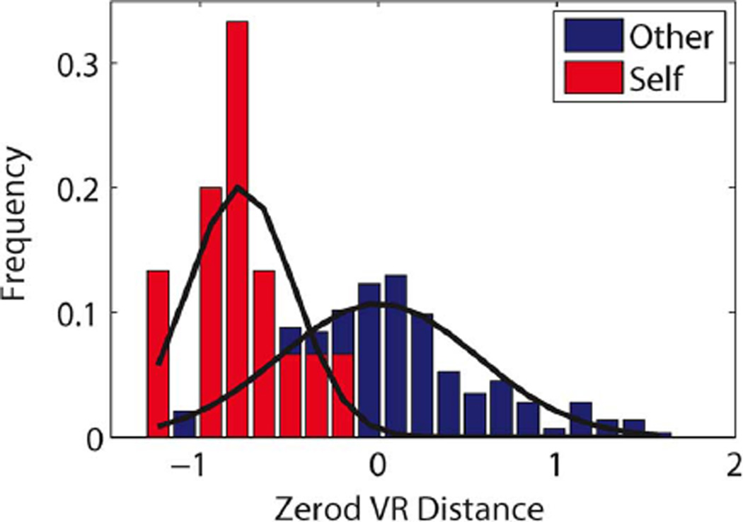
In order to apply the nonparametric estimators considered in this paper, we preprocessed the data first according to the following procedure: We convolved the observed spike trains with a decaying exponential of width τ = 5 ms; see [5] for more details. From the resulting smoothed responses, separately for each stimulus (i.e., each song), a template was formed based on nine out of the ten available responses. For the remaining response, convolved by the same decaying exponential, we then calculated the L₂ distances [also sometimes referred to as “van Rossum (VR) distance” in the neuroscience literature] to each of the templates, i.e., the distance to the correct template and the distances to the 19 incorrect templates. We repeated this procedure by using each possible subset of nine out of the ten responses to obtain the template, and the resulting histogram of distances is shown in Fig. 2. Below, the VR distances are used in two different ways to estimate the stimulus-response information.

Fig. 2.

Histogram of the (shifted) L₂ (VR) distances to the correct (self) and to the incorrect (other) templates, along with a simple Gaussian fit. The origin was artificially set to the mean of the distances to the incorrect templates.

C. “Confusion Information”

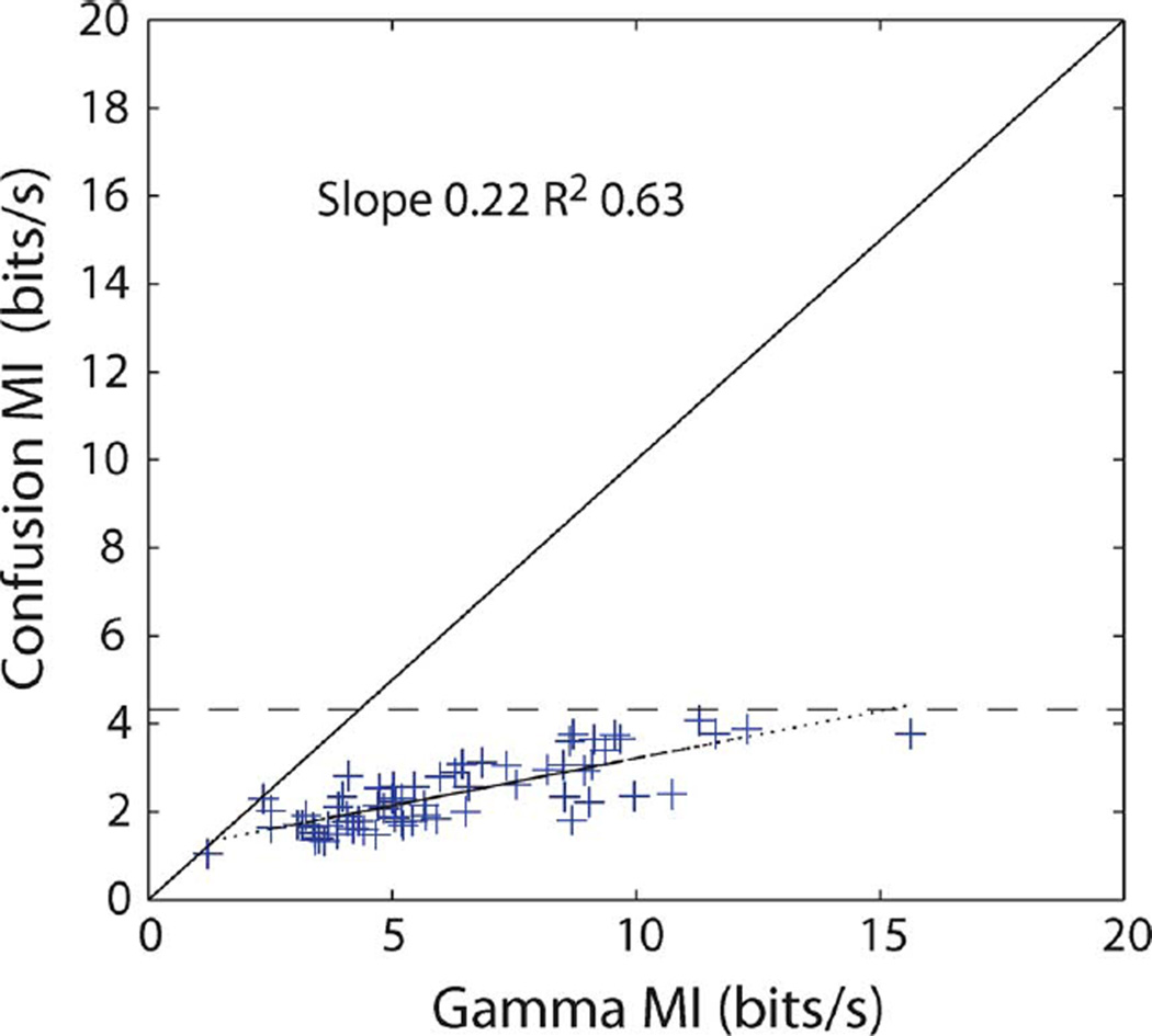
If the VR distances (as illustrated in Fig. 2) are used to “decode” the stimulus based on the observed response, we obtain a profile of correct and incorrect decoding and can use this to estimate information. More precisely, if the true stimulus is denoted by S and the decoded stimulus by Ŝ we estimate the MI I(S; Ŝ). Since there are only 20 different stimuli, it is immediately clear that this MI and any naive estimate thereof cannot exceed log₂(20) ≈ 4.32 bits. Fig. 3 compares the estimate ${Î}_{\alpha =0}^{(20)}$ to the information value calculated from the Gamma model, as described briefly in Section III-A. Each data point in the figure corresponds to one of the 66 neurons that were studied. The saturation effect is clearly visible.

Fig. 3.

“Confusion information” versus the gamma information. The confusion information underestimates the MI and is bounded by log₂(20) ≈ 4.32 bits, shown as a dotted line.

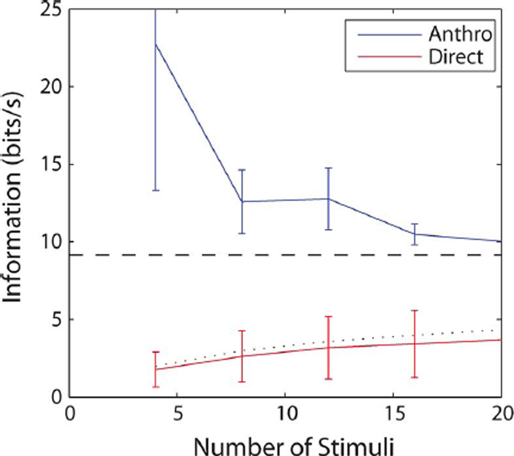
Fig. 4 illustrates the potential of the anthropically corrected estimator ${Î}_{\alpha =1}^{(K)}$ as compared to the naive estimator ${Î}_{\alpha =0}^{(K)}$ for increasing values of K, for a single neuron. As suggested by the properties that were theoretically derived in this paper, we see that ${Î}_{\alpha =1}^{(K)}$ is an upper bound, and ${Î}_{\alpha =0}^{(K)}$ a lower bound, to the “true” information. Recall that in this comparison, the information calculated from the Gamma model is considered the true information.

Fig. 4.

MI as a function of the number of stimuli obtained from the naive estimate (red) and from the anthropic correction. The dotted line shows the saturation bound of the naive estimate log₂(K). The dashed line is the gamma information for this neuron. This example corresponds to one of the best neurons both in terms of gamma information and in terms of the goodness of fit of the decoding algorithm; note that the naive estimate is very close to its theoretical (saturation) upper bound.

D. “Z-Information”: Fitting the Distributions With Gaussians

A practically interesting variation on the estimators presented here is to first fit simple distributions to the observed p(y|x_k) and p_k,α(y). Clearly, an obvious candidate is the Gaussian distribution. This is suggested in Fig. 2. In particular, the suggestion is to fit, separately for each k, a Gaussian distribution to the distribution p(y|x_k), with mean μ_k and variance ${\sigma }_k^2$ and another Gaussian distribution to the distribution p_k,α(y), with mean μ̃_k,α and variance ${\tilde{\sigma }}_{k,\alpha }^2$. For one particular x_k, these two Gaussian distributions are sketched in Fig. 2.

Then, the (modified) anthropically corrected estimator can be expressed as

$${Î}_{𝒩,\alpha }^{(K)}=\frac{1}{K\text{ln}2}\sum _{k=1}^K(\text{ln}\frac{{\tilde{\sigma }}_{k,\alpha }}{{\sigma }_k}+\frac{{({\tilde{\mu }}_{k,\alpha }-{\mu }_k)}^2}{2{\tilde{\sigma }}_{k,\alpha }^2}+\frac{{\sigma }_k^2-{\tilde{\sigma }}_{k,\alpha }^2}{{\tilde{\sigma }}_{k,\alpha }^2})$$ (13)

but it should be pointed out that this version no longer satisfies the basic properties derived in Section II. In particular, it is clear that as K → ∞, this estimator does not converge to the true information in general. Nevertheless, practically, this estimator should be expected to be interesting due to its inherent simplicity.

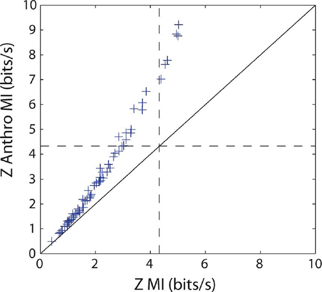
Fig. 5 compares the estimators ${Î}_{𝒩,\alpha =1}^{(20)}$ and ${Î}_{𝒩,\alpha =0}^{(20)}$ for all 66 neurons. It should be observed that ${Î}_{𝒩,\alpha =0}^{(K)}$, while no longer bounded by log₂(20) bits, nevertheless does not significantly exceed this bound, showing that the Gaussian assumption is reasonable in this example. Note also that the anthropic correction is again not subject to this saturation effect.

Fig. 5.

Z-dist anthropic estimate versus the Z-dist naive estimate of the MI. The dotted lines show log₂(20) ≈ 4.32 bits. The Z-dist information is approximately bounded by this value whereas the anthropic correction is not.

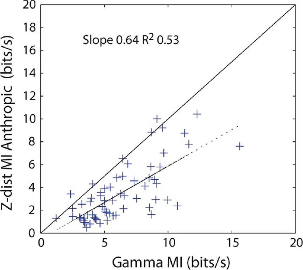
If the anthropic estimate is a better estimate of the MI, we postulate that it should be closer to the gamma information than the naive estimate. Comparing Figs. 3 and 6, it is clear that this is indeed the case. Note however also that for the vast majority of the neurons, the anthropic correction is still below the gamma information. This is due to the inherent suboptimality of the decoding approach in terms of VR distance considered here. If a better decoding approach, or the full probability distribution, was used, then the anthropic correction would match or exceed the gamma information.

Fig. 6.

Anthropic estimate of the MI after decoding the spike trains versus the gamma information.

IV. Application II: Redundancy Estimation

A. Measures of Neural Population Redundancy

Another context in which information measures have been advocated is the redundancy of neuronal ensembles. Several such measures have been proposed in the literature. Here, we will consider the following:

$$r\prime \stackrel{\text{def}}{=}\frac{{\sum }_{m=1}^{M}I(S;R_m)-I(S;R_1,R_2,\dots ,R_M)}{{\sum }_{m=1}^{M}I(S;R_m)}.$$ (14)

This measure has appeared in various forms in the literature, including in [27], [28], and [6]. Several properties of this measure can be established, such as the fact that r′ ≤ 1, but also that r′ can be negative (and even unboundedly so) for a code that would be referred to as “synergistic” in the neuroscience literature; see, e.g., [9].

B. Experimental Results

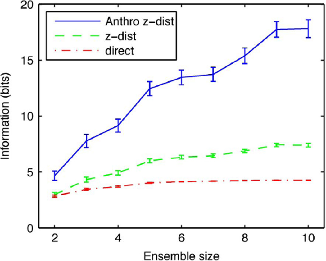
We examined the use of the anthropic correction for the estimation of the redundancy in an ensemble of neurons. For this purpose, we calculated VR distances between ensembles of trial spike trains and ensemble templates. This ensemble distance was taken to be the sum of the individual VR distances after normalization by the average distance between templates for the corresponding neuron. This normalization yielded a weighted average in which neurons that carried more information had larger weights than neurons that carried less information. As in the single neuron case, these ensemble distances can be used to generate a confusion matrix and a measure of MI (the confusion information). Alternatively, we computed the estimate of the MI directly from the distribution of distances fitted with Gaussians, i.e., the estimator ${Î}_{𝒩,\alpha }^{(K)}$ that was defined above in (13). Again, we compare the direct estimate ${Î}_{𝒩,\alpha =0}^{(K)}$ to the (full) anthropic correction ${Î}_{𝒩,\alpha =1}^{(K)}$. As can be seen in Fig. 7, the MI for an ensemble of neurons is quite sensitive to undersampling of the stimulus space. The confusion information saturates to its absolute upper bound (log₂(20)) for ensembles of five neurons or more; the fraction of correct stimulus classifications (obtained by the sum of the diagonal in the confusion matrix) is close to 100% in these cases. The smoothed estimate of the MI obtained by fitting the distribution of distances with Gaussians, which we denote by ${Î}_{𝒩,\alpha =0}^{(K)}$ (referred to as “Z MI” in the figure), also saturates. The anthropic estimate ${Î}_{𝒩,\alpha =1}^{(K)}$ (referred to as “Z Anthro MI” in the figure), on the other hand increases almost linearly. Given the results for single neurons (shown in Figs. 4 and 6), we believe that this anthropic estimate is a much better approximation of the actual ensemble MI.

Fig. 7.

MI for neuronal ensembles of two to ten neurons. The information is estimated from the confusion matrix (confusion MI), the distribution of distances modeled with Gaussians (Z MI) and with the anthropic correction for this estimate (Z anthro MI). The error bars show one standard error obtained by randomly sampling neurons from our data set.

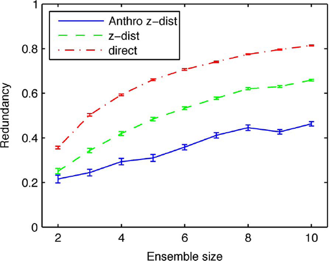
The effect of saturation will greatly affect the estimates of neural redundancy. In Fig. 8, we show the estimated redundancy using the measure r′ defined above in (14), calculated for the data shown in Fig. 7. The values of the redundancy obtained from the “confusion MI” would suggest a highly redundant neural code but the anthropic estimate shows a very different picture. Although the redundancy increases with the number of neurons, it does so slowly and, for ensembles with fewer than ten neurons, remains below 0.5. One would therefore conclude that sensory information is represented in a parallel fashion with restricted overlap in the information conveyed. These results illustrate the importance of lower and upper bounds in the MI calculation when it is applied to this type of problem.

Fig. 8.

Redundancy in information transmitted as a function of the number of neurons. The three curves for the redundancy are obtained from three estimates of the MI as explained in Fig. 7. The error bars show one standard error obtained by randomly sampling neurons from our data set.

V. Concluding Remarks

This paper introduces a novel information estimator called anthropic correction. Its most attractive application is in the asymmetric information estimation scenario where only a few samples are available of one of the two random variables, but for each of these samples, ample measurements of the other random variable are available. This is a common scenario for many existing data sets in neuroscience. The problem with this scenario is that a naive estimate is upper bounded by the logarithm of the smaller number of samples, which introduces a significant negative bias. To address this, we have introduced an anthropic correction which we proved has a nonnegative bias. Further properties of this estimator were established, and we illustrated that this novel estimate is very useful in sensory neurosciences where neuronal responses for a small number of stimuli or stimulus states are acquired for single neurons or ensembles of neurons. Both the estimates of the MI and of the redundancy in the information transmitted can be far from the actual values if a naive calculation is used. In those cases considering the anthropic correction could be crucial. The anthropic correction could also be useful for other systems with similar data limitations.

Biographies

Michael C. Gastpar (M’04) received the Dipl. El.-Ing. degree from the Swiss Federal Institute of Technology (ETH), Zürich, Switzerland, in 1997, the M.S. degree from the University of Illinois at Urbana-Champaign, Urbana, in 1999, and the Doctorat ès Science degree from the Swiss Federal Institute of Technology (EPFL), Lausanne, Switzerland, in 2002, all in electrical engineering. He was also a student in engineering and philosophy at the University of Edinburgh, Edinburgh, U.K., and the University of Lausanne.

He is currently an Associate Professor at the Department of Electrical Engineering and Computer Sciences, University of California, Berkeley, and a Full Professor in the Faculty of Electrical Engineering, Mathematics and Computer Science (EEMCS), Delft University of Technology, Delft, The Netherlands. He was a Summer Researcher at the Mathematics of Communications Department, Bell Labs, Lucent Technologies, Murray Hill, NJ. His research interests are in network information theory and related coding and signal processing techniques, with applications to sensor networks and neuroscience.

Dr. Gastparwon the 2002 EPFL Best Thesis Award, an NSF CAREER Award in 2004, and an Okawa Foundation Research Grant in 2008.

Patrick R. Gill received the B.Sc. degree (honors) from the University of Toronto, Toronto, ON, Canada, in 2001 and the Ph.D. degree from the University of California at Berkeley, Berkeley, in 2007.

He is currently Postdoctoral Researcher at the School of Electrical and Computer Engineering, Cornell University, Ithaca, NY. He was also a student in biophysics at the University of California at Berkeley, and a Summer Researcher at the Mathematics Department, University of Victoria, Victoria, BC, Canada. His research interests are in computational and theoretical neuroscience, with specialization in the fields of sensory neuroscience and neural network behaviors.

Dr. Gill won the 2007 Alan J. Bearden Award for an outstanding dissertation on a biophysical topic.

Alexander G. Huth received the B.S. and M.S. degrees from the California Institute of Technology, Pasadena, in 2007 and 2009, respectively.

Frédéric E. Theunissen received the B.S. degree in engineering physics and the Ph.D. degree in biophysics from the University of California at Berkeley, Berkeley, in 1985 and 1993, respectively.

He is currently an Associate Professor at the Department of Psychology and a member of the Helen Wills Neurosciences Institute at University of California at Berkeley. His research interests are in auditory science, computational neurosciences, and animal communication.

Dr. Theunissen, as an assistant professor, he was awarded a Sloan Fellowship in Theoretical Neuroscience (1999) and a Searle Fellowship for Biomedical Research (1999). He is a member of the Acoustical Society of America, the Neurosciences Society, and the International Neuroethological Society.

Appendix I

Proof of Lemma 1

The lower bound in part 1) follows directly from the fact that the Kullback–Leibler divergence is always nonnegative. The upper bound follows directly from

$${Î}_{\alpha }^{(K,n)}=\frac{1}{K}\sum _{k=1}^K\sum _{y\in 𝒴}\hat{p}(y|x=x_k){\text{log}}_2\frac{\hat{p}(y|x=x_k)}{{\hat{p}}_{k,\alpha }(y)}\le \frac{1}{K}\sum _{k=1}^K\sum _{y\in 𝒴}\hat{p}(y|x=x_k){\text{log}}_2\frac{\hat{p}(y|x=x_k)}{\frac{1-\alpha }{K}\hat{p}(y|x=x_k)}$$ (15)

since the logarithm is monotonically increasing. Part 2) can be proved using the following inequality [16, Th.2.7.2, p.32]:

$$𝔻(\lambda p_1+(1-\lambda )p_2\Vert \lambda q_1+(1-\lambda )q_2)\le \lambda 𝔻(p_1\Vert q_1)+(1-\lambda )𝔻(p_2\Vert q_2)$$ (16)

for 0 ≤ λ ≤ 1. For notational convenience, let us define p̂_k = p̂(r|s = s_k) and

$${\hat{p}}_{-k}=\frac{1}{K-1}\sum _{j=1,j\ne k}^K\hat{p}(r|s=s_j)$$ (17)

which can be used to express

$${\hat{p}}_{k,\alpha }(r)=\frac{1-\alpha }{K}\sum _{i=1}^K\hat{p}(r|s=s_i)+\frac{\alpha }{K-1}\sum _{j=1,j\ne k}^K\hat{p}(r|s=s_j)$$ (18)

$$=\frac{1-\alpha }{K}{\hat{p}}_k+(1-\frac{1-\alpha }{K}){\hat{p}}_{-k}$$ (19)

With this, we can express

$${Î}_{\alpha }^{(K,n)}=\frac{1}{K}\sum _{k=1}^K{𝔻}_{KL}({\hat{p}}_k\Vert \frac{1-\alpha }{K}{\hat{p}}_k+(1-\frac{1-\alpha }{K}\left){\hat{p}}_{-k}\right)$$ (20)

$$=\frac{1}{K}\sum _{k=1}^K{𝔻}_{KL}({\hat{p}}_k\Vert \frac{\epsilon }{K}{\hat{p}}_k+\frac{1-\alpha -\epsilon }{K}{\hat{p}}_k+(1-\frac{1-\alpha }{K}\left){\hat{p}}_{-k}\right)$$ (21)

Next, in each term inside the sum separately, we can use (16) with p₁ = p₂ = q₁ = p̂_k and q₂ = (1 − α − ε)/[K(1 − ε/K]p̂_k + (1 − (1 − α)/K)/(1 − ε/K)p̂−k, and λ = ε/K. Thus, we find the following bound:

$${Î}_{\alpha }^{(K,n)}\le \frac{1}{K}\sum _{k=1}^K(1-\frac{\epsilon }{K}){𝔻}_{KL}\times ({\hat{p}}_r\Vert \frac{1-\alpha -\epsilon }{K(1-\epsilon /K)}{\hat{p}}_r+\frac{1-(1-\alpha )/K}{1-\epsilon /K}{\hat{p}}_{-k}(r))$$ (22)

$$=(1-\frac{\epsilon }{K}){Î}_{\alpha \prime }^{(K)}$$ (23)

with

$$\alpha \prime =\frac{(K-1)\epsilon /K+\alpha }{1-\epsilon /K}.$$ (24)

To conclude the argument, we can use the last equation to find ε as a function of α and α′ as

$$\frac{\epsilon }{K}=\frac{\alpha \prime -\alpha }{K-1+\alpha \prime }$$ (25)

which is the claimed formula.

Appendix II

Proof of Theorem 1

The lower bound in Theorem 1 follows directly from the observation that ${Î}_{\alpha =0}^{(K)}$ is a MI, namely, for a fixed conditional distribution (channel) given by p(y|x) and an input distribution that consists of K randomly selected points of the true distribution p(x). We can write

$$𝔼\left[{Î}_{\alpha }^{(K)}\right]=\sum _{x_1,x_2,\dots ,x_K}{p}_X(x_1)\cdots p_X(x_K)\times [\frac{1}{K}\sum _{k=1}^K{𝔻}_{KL}(p_{Y|X}(y|x=x_k)\Vert p_{k,0}(y))]$$ (26)

$$=𝔼\left[I\right(p^{(K)}(x),p(y|x))]$$ (27)

where p^(K)(x) denotes the distribution supported on K randomly chosen points of the true p(x), and the expectation is over this choice. Since MI is concave in the input distribution for fixed conditional distribution [16, Th. 2.7.4], we can conclude from Jensen’s inequality that

$$𝔼\left[I\right(p^{(K)}(x),p(y|x))]\le I(𝔼[p^{(K)}(x)],p(y|x))=I(X;Y).$$ (28)

For the upper bound in Theorem 1, we will establish the slightly stronger result that $𝔼[{Î}_1^{(K,n)}]$ is no smaller than the true information for any value of n, not only in the limit as n → ∞, as follows:

$$𝔼\left[{Î}_1^{(K,n)}\right]=\sum _{x_1,x_2,\dots ,x_K}p(x_1)\cdots p(x_K)\times \sum _{y_{1,1},\dots ,y_{K,n}}p(y_{1,1}|x_1)\cdots p(y_{K,n}|x_K)\times [\frac{1}{K}\sum _{k=1}^K{𝔻}_{KL}(\hat{p}(y|x=x_k)\Vert {\hat{p}}_{k,\alpha =1}(y))].$$

But from the log-sum inequality [16, Th. 2.7.1], we have that

$$\sum _{y_{1,1},\dots ,y_{K,n}}p(y_{1,1}|x_1)\cdots p(y_{K,n}|x_K)\times {𝔻}_{KL}(\hat{p}(y|x=x_k)\Vert {\hat{p}}_{k,\alpha =1}(y))=\sum _{y\in 𝒴}\sum _{y_{1,1},\dots ,y_{K,n}}p(y_{1,1}|x_1)\cdots p(y_{K,n}|x_K)\times \hat{p}(y|x=x_k){\text{log}}_2\frac{\hat{p}(y|x=x_k)}{{\hat{p}}_{k,\alpha =1}(y)}$$ (29)

$$\ge \sum _{y\in 𝒴}(\sum _{y_{1,1},\dots ,y_{K,n}}p(y_{1,1}|x_1)\cdots p(y_{K,n}|x_K)\hat{p}(y|x=x_k))\times {\text{log}}_2\frac{{\sum }_{y_{1,1},\dots ,y_{K,n}}p(y_{1,1}|x_1)\cdots p(y_{K,n}|x_K)\hat{p}(y|x=x_k)}{{\sum }_{y_{1,1},\dots ,y_{K,n}}p(y_{1,1}|x_1)\cdots p(y_{K,n}|x_K){\hat{p}}_{k,\alpha =1}(y)}$$ (30)

$${𝔻}_{KL}(p(y|x=x_k)\Vert {\tilde{p}}_{k,\alpha =1}(y))$$ (31)

where the last equality follows because the expected value of the histogram is the true probability mass function, irrespective of the number of samples n, and where we have used the following shorthand:

$${\tilde{p}}_{k,\alpha =1}(y)=\frac{1}{K-1}\sum _{j=1,j\ne k}^{K}p(y|x=x_j).$$ (32)

Thus, we have

$$𝔼\left[{Î}_1^{(K,n)}\right]\ge \sum _{x_1,x_2,\dots ,x_K}p(x_1)\cdots p(x_K)\times [\frac{1}{K}\sum _{k=1}^K{𝔻}_{KL}(p(y|x=x_k)\Vert {\tilde{p}}_{k,\alpha =1}(y))]=\frac{1}{K}\sum _{k=1}^K(\sum _{y\in 𝒴}\sum _{x_1,x_2,\dots ,x_K}p(x_1)\cdots p(x_K)\times p(y|x=x_k){\text{log}}_2\frac{p(y|x=x_k)}{{\tilde{p}}_{k,\alpha =1}(y)}).$$ (33)

Now, let us consider the first term in the outermost sum, i.e., for k = 1, namely

$$\sum _{y\in 𝒴}\sum _{x_1,x_2,\dots ,x_K}p(x_1)\cdots p(x_K)p(y|x=x_1){\text{log}}_2\frac{p(y|x=x_1)}{{\tilde{p}}_{1,\alpha =1}(y)}=\sum _{y\in 𝒴}\sum _{x_1,x_2,\dots ,x_K}p(x_1)\cdots p(x_K)\times p(y|x=x_1){\text{log}}_2\frac{p(y|x=x_1)}{\frac{1}{K-1}{\sum }_{j=2}^{K}p(y|x=x_j)}$$ (34)

$$=\sum _{y\in 𝒴}\sum _{x_1}p(x_1)\sum _{x_2,x_3,\dots ,x_K}p(x_2)\cdots p(x_K)\times p(y|x=x_1){\text{log}}_2\frac{p(x_2)\cdots p(x_K)p(y|x=x_1)}{p(x_2)\cdots p(x_K)\frac{1}{K-1}{\sum }_{j=2}^{K}p(y|x=x_j)}$$ (35)

where the last step is a trivial manipulation. Now, we can lower bound the second sum using the log-sum inequality [16, Th. 2.7.1], as follows:

$$\sum _{x_2,x_3,\dots ,x_K}p(x_2)\cdots p(x_K)p(r|s=s_1)\times {\text{log}}_2\frac{p(s_2)\cdots p(s_K)p(y|x=x_1)}{p(x_2)\cdots p(x_K)\frac{1}{K-1}{\sum }_{j=2}^{K}p(y|x=x_j)}\ge (\sum _{x_2,x_3,\dots ,x_K}p(x_2)\cdots p(x_K)p(y|x=x_1))\times {\text{log}}_2\frac{{\sum }_{x_2,x_3,\dots ,x_K}p(x_2)\cdots p(x_K)p(y|x=x_1)}{{\sum }_{x_2,x_3,\dots ,x_K}p(x_2)\cdots p(x_K)\frac{1}{K-1}{\sum }_{j=2}^{K}p(y|x=x_j)}=p(y|x=x_1){\text{log}}_2\frac{p(y|x=x_1)}{p(y)}$$ (36)

Thus, we find

$$\sum _{y\in 𝒴}\sum _{x_1,x_2,\dots ,x_K}p(x_1)\cdots p(x_K)p(y|x=x_1){\text{log}}_2\frac{p(y|x=x_1)}{{\hat{p}}_{1,\alpha =1}(y)}\ge \sum _{y\in 𝒴}\sum _{x_1}p(x_1)p(y|x=x_1){\text{log}}_2\frac{p(y|x=x_1)}{p(y)}$$ (37)

$$=I(X;Y).$$ (38)

Proceeding by analogy, we find the same bound for k = 2, 3, …, K, establishing the claim.

Appendix III

Definition 2

For a fixed collection of K samples from X, denoted by {x₁, x₂, …, x_K}, let yⁿ denote the length-n sequence of vectors y_i = (y_{1, j}, y_{2, j}, …, y_{K, j})^T. Define the set

$$A_{\epsilon }^{(n)}=\{{\mathbf{y}}^n:{\cap }_{k=1}^K\{|\hat{p}(y|x_k)-p(y|x_k)|\le \epsilon p(y|x_k),\forall y\in 𝒴\}\}$$ (39)

where p̂(y|x_k) is the histogram estimate based on ${\{y_{k,j}\}}_{j=1}^n$.

This is sometimes referred to as robust typicality; see, e.g., [29]. Merely for notational convenience, we also define

$${\widehat{𝔻}}_{k,\alpha }^{(n)}=𝔻(\hat{p}(y|x_k)\Vert {\hat{p}}_{k,\alpha }(y))$$ (40)

$${𝔻}_{k,\alpha }=𝔻(p(y|x_k)\Vert p_{k,\alpha }(y)).$$ (41)

Note that with this definition

$${Î}_{\alpha }^{(K,n)}=\frac{1}{K}\sum _{k=1}^K{\widehat{𝔻}}_{k,\alpha }^{(n)}.$$ (42)

Lemma 2

If Yⁿ are sampled i.i.d. from the distribution ${\prod }_{k=1}^{K}p(y_k|x=x_k)$, then with p_min(y|x_k) = min_y p(y|x_k)

$$\mathbb{P}({\mathbf{Y}}^n\in A_{\epsilon }^{(n)})\ge 1-\frac{1}{n{\epsilon }^2}\sum _{k=1}^K\frac{|𝒴|}{p_{\text{min}}^2(y|x_k)}.$$ (43)

Proof

This proof is standard up to the fact that Y is a vector and we enforce (robust) typicality in each component

$$\mathbb{P}({\mathbf{Y}}^n\in A_{\epsilon }^{(n)})=1-\mathbb{P}({\mathbf{Y}}^n\in \{{\mathbf{y}}^n:{\cup }_{k=1}^K\{|\hat{p}(y|x_k)-p(y|x_k)|>\epsilon p(y|x_k)\}\})$$ (44)

$$\ge 1-\sum _{k=1}^K\mathbb{P}({\mathbf{Y}}^n\in \{{\mathbf{y}}^n:|\hat{p}(y|x_k)-p(y|x_k)|>\epsilon p(y|x_k)\})$$ (45)

where the last step is the union bound. To complete the proof, we use the Chebyshev inequality to upper bound each term in the sum, separately for each value of y ∈ 𝒴, like in e.g., [30, Th. 1.2.12].

Lemma 3

For any ${\mathbf{y}}^n\in A_{\epsilon }^{(n)}$, any k = 1, 2, …, L, any 0 ≤ α ≤ 1, and any 0 < ε < 1/2, we have

$$|{\widehat{𝔻}}_{k,\alpha }^{(n)}-{𝔻}_{k,\alpha }|\le \epsilon ({𝔻}_{k,\alpha }+6)$$ (46)

Proof

Since we assume ${\mathbf{y}}^n\in A_{\epsilon }^{(n)}$, we know that |p̂(y|x_k) − p(y|x_k)| ≤ εp(y|x_k). Note that this implies that |p̂_k,α(y) − p_k,α(y)| ≤ εp_k,α(y). Maximizing ${\widehat{𝔻}}_{k,\alpha }^{(n)}$ over all p̂(y|x_k) that satisfy this condition, we find the following upper bound:

$${\widehat{𝔻}}_{k,\alpha }^{(n)}\le \sum _y(1+\epsilon )p(y|x_k)\text{log}\frac{(1+\epsilon )p(y|x_k)}{(1-\epsilon )p_{k,\alpha }(y)}.$$ (47)

By analogy, minimizing ${\widehat{𝔻}}_{k,\alpha }^{(n)}$ over all p̂(y|x_k) that satisfy this condition, we find the following lower bound:

$${\widehat{𝔻}}_{k,\alpha }^{(n)}\ge \sum _y(1-\epsilon )p(y|x_k)\text{log}\frac{(1-\epsilon )p(y|x_k)}{(1+\epsilon )p_{k,\alpha }(y)}.$$ (48)

Clearly, $|{\widehat{𝔻}}_{k,\alpha }^{(n)}-{𝔻}_{k,\alpha }|\le \text{max}\{{\widehat{𝔻}}_{k,\alpha }^{(n)}-{𝔻}_{k,\alpha },{𝔻}_{k,\alpha }-{\widehat{𝔻}}_{k,\alpha }^{(n)}\}$. Finally, noting that for 0 < ε < 1/2, we have $(1+\epsilon )\text{log}\frac{1+\epsilon }{1-\epsilon }\le 6\epsilon$, we obtain the claimed bound.

Proof of Theorem 2

We begin by considering

$$\mathbb{P}\left(\right|{Î}_{\alpha }^{(K,n)}-{Î}_{\alpha }^{(K)}|>\epsilon (D_{\text{max},\alpha }+6))=\mathbb{P}\left(\right|\frac{1}{K}\sum _{k=1}^K({\widehat{𝔻}}_{k,\alpha }^{(K,n)}-{𝔻}_{k,\alpha }^{(K)})|>\epsilon (D_{\text{max},\alpha }+6)).$$ (49)

However, the event can only occur if for at least one of the k, we have $|{\widehat{𝔻}}_{k,\alpha }^{(K,n)}-{𝔻}_{K,\alpha }^{(K)}|>\epsilon (D_{\text{max},\alpha }+6)$. Thus, by the union bound

$$\mathbb{P}\left(\right|{Î}_{\alpha }^{(K,n)}-{Î}_{\alpha }^{(K)}|>\epsilon (D_{\text{max},\alpha }+6))\le \sum _{k=1}^K\mathbb{P}\left(\right|{\widehat{𝔻}}_{k,\alpha }^{(K,n)}-{𝔻}_{k,\alpha }^{(K)}|>\epsilon (D_{\text{max},\alpha }+6)).$$ (50)

To conclude the argument, we can now use Lemma 3 and the fact that D_max,α ≥ 𝔻_k,α

$$\mathbb{P}\left(\right|{\widehat{𝔻}}_{k,\alpha }^{(n)}-{𝔻}_{k,\alpha }|\le \epsilon (D_{\text{max},\alpha }+6))\ge \mathbb{P}({\mathbf{Y}}^n\in A_{\epsilon }^{(n)})\ge 1-\frac{1}{n{\epsilon }^2}\sum _{k=1}^K\frac{|𝒴|}{p_{\text{min}}^2(y|x_k)}$$ (51)

where the last inequality follows from Lemma 2.

Lemma 4

For any k = 1, 2, …, L, and any 0 ≤ α < 1

$$𝔼\left[{({\widehat{𝔻}}_{k,\alpha }^{(n)}-{𝔻}_{k,\alpha })}^2\right]\le \frac{C}{\sqrt{n}}.$$ (52)

Proof

We use a standard truncation argument

$$𝔼\left[{({\widehat{𝔻}}_{k,\alpha }^{(n)}-{𝔻}_{k,\alpha })}^2\right]=\mathbb{P}({\mathbf{Y}}^n\in A_{\epsilon }^{(n)})𝔼\left[{({\widehat{𝔻}}_{k,\alpha }^{(n)}-{𝔻}_{k,\alpha })}^2\right|{\mathbf{Y}}^n\in A_{\epsilon }^{(n)}]+\mathbb{P}({\mathbf{Y}}^n\notin A_{\epsilon }^{(n)}\left)𝔼\right[{({\widehat{𝔻}}_{k,\alpha }^{(n)}-{𝔻}_{k,\alpha })}^2|{\mathbf{Y}}^n\notin A_{\epsilon }^{(n)}].$$ (53)

Clearly, from Lemma 3, we have

$$𝔼\left[{({\widehat{𝔻}}_{k,\alpha }^{(n)}-{𝔻}_{k,\alpha })}^2\right|{\mathbf{Y}}^n\in A_{\epsilon }^{(n)}]\le {\epsilon }^2{(D_{\text{max},\alpha }+6)}^2.$$ (54)

Moreover, from Lemma 2

$$\mathbb{P}({\mathbf{Y}}^n\notin A_{\epsilon }^{(n)})\le \frac{1}{n{\epsilon }^2}\sum _{k=1}^K\frac{|𝒴|}{p_{\text{min}}^2(y|x_k)}.$$ (55)

Thus

$$𝔼\left[{({\widehat{𝔻}}_{k,\alpha }^{(n)}-{𝔻}_{k,\alpha })}^2\right]\le {\epsilon }^2{(D_{\text{max},\alpha }+6)}^2+\frac{1}{n{\epsilon }^2}\sum _{k=1}^K\frac{|𝒴|}{p_{\text{min}}^2(y|x_k)}({\hat{D}}_{\text{max},\alpha }^2+D_{\text{max},\alpha }^2)$$ (56)

where we have used the fact that α < 1 to obtain a bound ${\hat{D}}_{\text{max},\alpha }={\text{log}}_2\frac{K}{1-\alpha }$; see Lemma 1. Finally, selecting ${\epsilon }^2=1/\sqrt{n}$ gives the desired result.

Proof of Theorem 3

The theorem follows directly from Lemma 4 by noting that

$$𝔼\left[{({Î}_{\alpha }^{(K,n)}-{Î}_{\alpha }^{(K)})}^2\right]=𝔼\left[{(\frac{1}{K}\sum _{k=1}^K{\widehat{𝔻}}_{k,\alpha }^{(n)}-{𝔻}_{k,\alpha })}^2\right]\le \underset{k}{\text{max}}𝔼\left[{({\widehat{𝔻}}_{k,\alpha }^{(n)}-{𝔻}_{k,\alpha })}^2\right]$$ (57)

which completes the proof.

References

- 1.Borst A, Theunissen FE. Information theory and neural coding. Nature Neurosci. 1999 Nov;2:947–957. doi: 10.1038/14731. [DOI] [PubMed] [Google Scholar]
- 2.Rieke F, Warland D, de Ruyter van Steveninck RR, Bialek W. Spikes: Exploring the Neural Code. Cambridge, MA: MIT Press; 1997. [Google Scholar]
- 3.Globerson A, Stark E, Vaadia E, Tishby N. The minimum information principle and its application to neural code analysis. Proc. Nat. Acad. Sci. USA. 2009 Mar;106:3490–3495. doi: 10.1073/pnas.0806782106. [DOI] [PMC free article] [PubMed] [Google Scholar]
- 4.Rieke F, Bodnar DA, Bialek W. Naturalistic stimuli increase the rate and efficiency of information transmission by primary auditory afferents. Proc. R. Soc. Lond. B, Biol. Sci. 1995;262(1365):259–265. doi: 10.1098/rspb.1995.0204. [DOI] [PubMed] [Google Scholar]
- 5.Hsu A, Woolley SMN, Fremouw TE, Theunissen FE. Modulation power and phase spectrum of natural sounds enhance neural encoding performed by single auditory neurons. J Neurosci. 2004 Oct;24:9201–9211. doi: 10.1523/JNEUROSCI.2449-04.2004. [DOI] [PMC free article] [PubMed] [Google Scholar]
- 6.Nelken I, Chechik G, Mrsic-Flogel TD, King AJ, Schnupp JWH. Encoding stimulus information by spike numbers and mean response time in primary auditory cortex. J Comput. Neurosci. 2005;19:199–221. doi: 10.1007/s10827-005-1739-3. [DOI] [PubMed] [Google Scholar]
- 7.Theunissen FE, Miller JP. Representation of sensory information in the cricket cercal sensory system. II. information theoretic calculation of system accuracy and optimal tuning-curve widths of four primary interneurons. J Neurophysiol. 1991;66(5):1690–1703. doi: 10.1152/jn.1991.66.5.1690. [DOI] [PubMed] [Google Scholar]
- 8.Dan Y, Attick JJ, Reid RC. Efficient coding of natural scenes in the lateral geniculate nucleus: Experimental test of a computational theory. J Neurosci. 1996;16:3351–3362. doi: 10.1523/JNEUROSCI.16-10-03351.1996. [DOI] [PMC free article] [PubMed] [Google Scholar]
- 9.Schneidman E, Bialek W, Berry MJ., II Synergy, redundancy, and independence in population codes. J Neurosci. 2003;23(37):11539–11553. doi: 10.1523/JNEUROSCI.23-37-11539.2003. [DOI] [PMC free article] [PubMed] [Google Scholar]
- 10.Narayanan N, Kimchy E, Laubach M. Redundancy and synergy of neuronal ensembles in motor cortex. J Neurosci. 2005;25:4207–4216. doi: 10.1523/JNEUROSCI.4697-04.2005. [DOI] [PMC free article] [PubMed] [Google Scholar]
- 11.Puchalla JR, Schneidman E, Harris RA, Berry MJ. Redundancy in the population code of the retina. Neuron. 2005;46(3):493–504. doi: 10.1016/j.neuron.2005.03.026. [DOI] [PubMed] [Google Scholar]
- 12.Chechik G, Anderson MJ, Bar-Yosef O, Young ED, Tishby N, Nelken I. Reduction of information redundancy in the ascending auditory pathway. Neuron. 2006;51:359–368. doi: 10.1016/j.neuron.2006.06.030. [DOI] [PubMed] [Google Scholar]
- 13.Paninski L. Estimation of entropy and mutual information. Neural Comput. 2003;15(6):1191–1253. [Google Scholar]
- 14.Averbeck BB, Latham PE, Pouget A. Neural correlations, population coding and computation. Nature Rev. Neurosci. 2006 May;7:358–366. doi: 10.1038/nrn1888. [DOI] [PubMed] [Google Scholar]
- 15.Gordona N, Shackletonb TM, Palmerb AR, Nelken I. Responses of neurons in the inferior colliculus to binaural disparities: Insights from the use of fisher information and mutual information. J Neurosci. Methods. 2008 Apr;169:391–404. doi: 10.1016/j.jneumeth.2007.11.005. [DOI] [PubMed] [Google Scholar]
- 16.Cover TM, Thomas JA. Elements of Information Theory. 2nd ed. New York: Wiley; 2006. [Google Scholar]
- 17.Carter B. Proc. IAU Symp. 63, Confrontation of Cosmological Theories With Observational Data. Dordrecht; 1974. Large number coincidences and the anthropic principle in cosmology; pp. 291–298. [Google Scholar]
- 18.Nguyen X, Wainwright MJ, Jordan MI. Proc. IEEE Int. Symp. Inf. Theory. France: Nice; 2007. Jun, Nonparametric estimation of the likelihood ratio and divergence functionals; pp. 2016–2020. [Google Scholar]
- 19.Wang Q, Kulkarni SR, Verdú S. Divergence estimation of continuous distributions based on data-dependent partitions. IEEE Trans. Inf. Theory. 2005 Sep;51(9):3064–3074. [Google Scholar]
- 20.Victor J, Purpura K. Estimation of information in neuronal responses. Trends Neurosci. 1999;22(12):543. doi: 10.1016/s0166-2236(99)01493-9. [DOI] [PubMed] [Google Scholar]
- 21.Victor JD. Binless strategies for estimation of information from neural data. Phys. Rev. E, Stat. Phys. Plasmas Fluids Relat. Interdiscip. Top. 2002;66:51903. doi: 10.1103/PhysRevE.66.051903. [DOI] [PubMed] [Google Scholar]
- 22.Panzeri S, Treves A. Analytical estimates of limited sampling biases in different information measures. Network, Comput. Neural Syst. 1996;(7):87–107. doi: 10.1080/0954898X.1996.11978656. [DOI] [PubMed] [Google Scholar]
- 23.Vu VQ, Yu B, Kass RE. Coverage-adjusted entropy estimation. Stat. Med. 2007;26(21):4039–4060. doi: 10.1002/sim.2942. [DOI] [PubMed] [Google Scholar]
- 24.Efron B. The Jackknife, the Bootstrap and Other Resampling Plans. Philadelphia, PA: SIAM; 1992. [Google Scholar]
- 25.Antos A, Kontoyiannis I. Convergence properties of functional estimates for discrete distributions. Random Structures Algorithms. 2001 Oct;19:163–193. [Google Scholar]
- 26.Strong SP, Koberle R, de Ruyter van Steveninck RR, Bialek W. Entropy and information in neural spike trains. Phys. Rev. Lett. 1998;80:197–200. [Google Scholar]
- 27.Reich DS, Mechler F, Victor JD. Independent and redundant information in nearby cortical neurons. Science. 2001;294:2566–2568. doi: 10.1126/science.1065839. [DOI] [PubMed] [Google Scholar]
- 28.Machens CK, Stemmler MB, Prinz P, Krahe R, Ronacher B, Herz AVM. Representation of acoustic communication signals in insect auditory receptors. J Neurosci. 2001;21(9):3215–3227. doi: 10.1523/JNEUROSCI.21-09-03215.2001. [DOI] [PMC free article] [PubMed] [Google Scholar]
- 29.Orlitsky A, Roche JR. Coding for computing. IEEE Trans. Inf. Theory. 2001 Mar;47(2):903–917. [Google Scholar]
- 30.Csiszár I, Körner J. Information Theory: Coding Theorems for Discrete Memoryless Systems. New York: Academic; 1982. [Google Scholar]